
Adsorption on Fractal Surfaces: A Non Linear Modeling Approach of a Fractional Behavior

IMS Laboratory, Bordeaux University, UMR CNRS 5218—351, Cours de la Libération, 33400 Talence, France
*
Authors to whom correspondence should be addressed.
Fractal Fract. 2021, 5(3), 65; https://0-doi-org.brum.beds.ac.uk/10.3390/fractalfract5030065
Submission received: 23 June 2021
/
Revised: 6 July 2021
/
Accepted: 7 July 2021
/
Published: 10 July 2021
(This article belongs to the Special Issue Fractional Behavior in Nature 2021)
Abstract
:This article deals with the random sequential adsorption (RSA) of 2D disks of the same size on fractal surfaces with a Hausdorff dimension . According to the literature and confirmed by numerical simulations in the paper, the high coverage regime exhibits fractional dynamics, i.e., dynamics in where d is the fractal dimension of the surface. The main contribution this paper is that it proposes to capture this behavior with a particular class of nonlinear model: a driftless control affine model.
1. Introduction
Adsorption is a widely encountered phenomenon, especially in physics, chemistry or biology, e.g., to capture pollutants [1,2], for water purification [3], or in gas sensors [4,5]. From a mathematical point of view, the idealized adsorption process is known as random sequential adsorption (RSA) which produces fractional behaviors.
RSA has been widely studied in the literature especially in 2 dimensions. There are results on the final jamming value [6,7,8], and on the kinetic of the density of free spaces which exhibits a behavior [6,9,10]. Numerous models have been proposed to capture this kinetic. An interesting analysis of these models is proposed in [11]. If denotes the amount of adsorbed particles, most of the models discussed express the adsorption rate as a function of the difference , where denotes the amount of particles adsorbed at equilibrium. The following models have been proposed: by Lagergren in 1898 [12]: ; by Kopelman in 1988 [13]: ; by Ho and Mckay in 2000 [14]: ; and by Brouers and Sotolongo-Costain in 2006 [15]:
If denotes the coverage density, where is the maximum amount of adsorbed particles and if c denotes the concentration of particles close to the surface (bulk), the following model was also proposed by Haerifar and Azizian in 2012 [16] and Bashiri and Shajari in 2014 [11]:
However, the RSA process is non-linear. If the flow of particles is doubled, the filling dynamic of the surface is almost doubled, but the final value is the same as for a single flow. Moreover, if the flow is stopped then the filling is obviously stopped as well. Furthermore, if the flow restarts, the filling will restart at the same point. Thus, none of the time varying and fractional models previously cited permit a consistent modeling of the RSA phenomenon. That is why a nonlinear model is proposed by the authors of [17].
In practice, the surface on which the adsorption occurs is not absolutely flat, which leads some authors to consider RSA on fractal surfaces [18]. Analysis of RSA on fractal surfaces has produced a major result: the high coverage regime exhibits a fractional behavior depending on the surface dimension d, i.e., dynamics in [6,9,18]. Such a property is in accordance with the analysis proposed in [19,20], which leads the author of [20] to claim that a kinetic in on space of dimension 1 produces a kinetic in on space of dimension d. This is precisely what we observe with the RSA process whose kinetic of free places density for the high coverage regime exhibits a behavior in 1D [21]. Physical examples of adsorption on fractal surfaces are also considered in numerous studies [22,23,24,25,26].
In line with reference [17], the main contribution of the present paper is that it proposes to capture the RSA kinetics on fractal surfaces with driftless control affine nonlinear models. An example of a driftless control-affine system is the nonholonomic integrator introduced in [27]. This class of system some times referred to as Brockett’s system, or the Heisenberg system, as it also arises in quantum mechanics [28]. Analysis and control results for this class of systems can be found in [29,30]. Two models are proposed: a simple one which is proved analytically to produce a fractional dynamic behavior and a more complex and accurate one. The accuracy of the latter model was assessed via numerical simulations on three types of fractal surfaces.
2. Evidence of the Fractional Asymptotic Behavior of Some Fractal Surfaces
This article deals with the random sequential adsorption (RSA) of 2D disks on a fractal surface. A definition of RSA is now given.
Definition 1 (RSA).
Random sequential adsorption is a process in which particles are constantly trying to attach themselves to a random location on a surface. If the incoming particle does not overlap any previously attached particles, then it binds irreversibly.
In order to model the phenomenon of physical adsorption, the random sequential adsorption model was used. For any surface, it is suggested in the literature [6,18] that the long time coverage density of the RSA follows a power law:
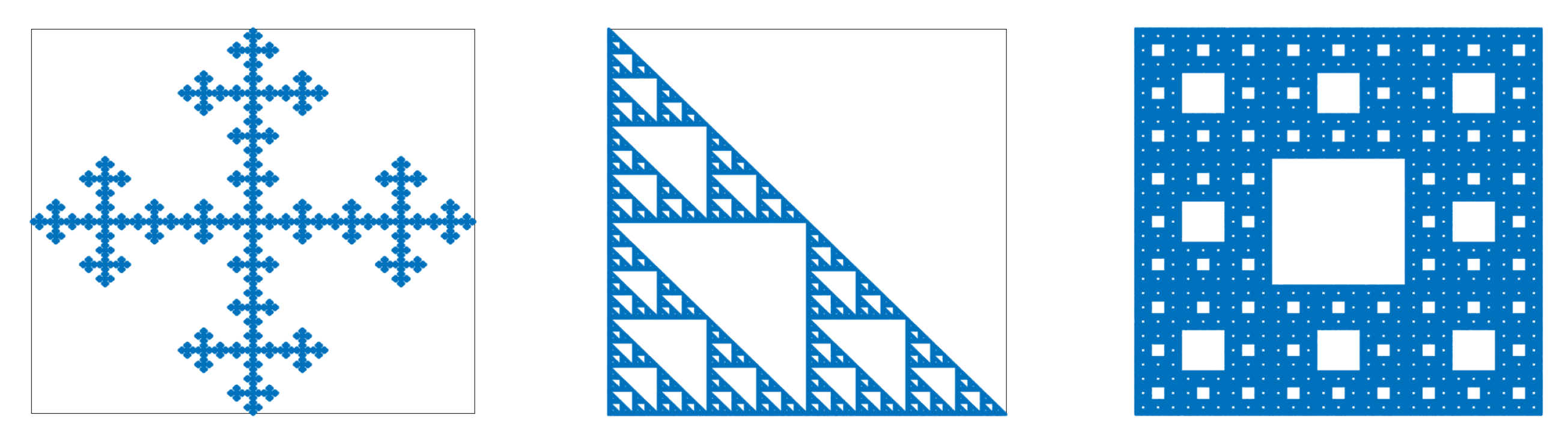
where d is the Hausdorff dimension of the surface on which the 2D disks arise. The fractal surfaces considered are a set of points contained in the square .
In order to simulate the RSA process of 2D disks on a given fractal surface, the RSA algorithm used is the same as in [17] and is recalled in Algorithm 1:
| Algorithm 1 Random Sequential Adsorption |
A random point of the fractal is selected at each iteration of the process. A disc of radius R and center c will fix on the surface if:
|
The fractal surfaces considered are illustrated in Figure 1.
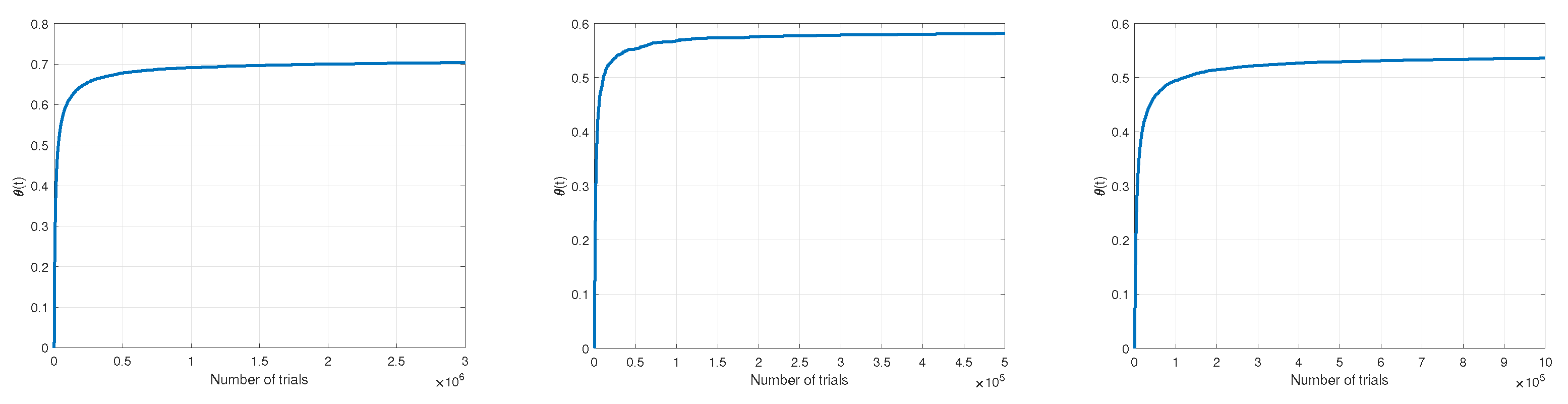
For each of the fractal surfaces previously cited, a RSA process was performed. As shown in [18], the asymptotic value of the density depends on the number of iterations in the fractal building process. The number of iterations needed to have relevant results seems to be greater than 6. The final values given in Table 1 are those proposed in [18] and are close to those plotted in Figure 2. The differences can be explained by differences in the simulation conditions (the number of iterations in the fractal building process, the number of trials, the ratio between the size of the disks and the size of the fractal).
The densities of adsorbed disks as a function of time (number of trials) for each of the considered fractals are shown in Figure 2.
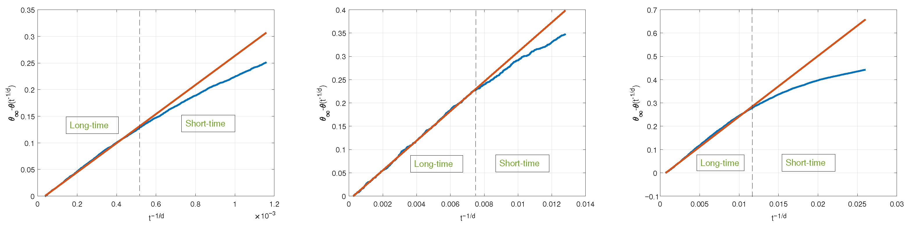
Figure 3 shows as a function of , where d is the dimension of the fractal. This figure provides evidence that the density of adsorbed disks has a power-law asymptotic behavior of the form
where d is the fractal surface dimension (Hausdorff dimension). The Hausdorff dimension of the Vicsek fractal is , for the Sierpinski triangle, for the Sierpinski carpet. The straight line on each subfigure of Figure 3 is the plot of to highlight the fractional behavior.
Figure 3 confirms that the results of the simulations are consistent with the expected power-law behaviors.
3. Power-Law Non Linear Dynamical Modeling
3.1. Detailed Modeling Approach on the Vicsek Fractal
In this section, the class of model considered is called a driftless control affine nonlinear model [27,28] and the first one is defined by the relation
can be viewed as an input and x(t) is the model state and output. , and (). This model produces trajectories of the form
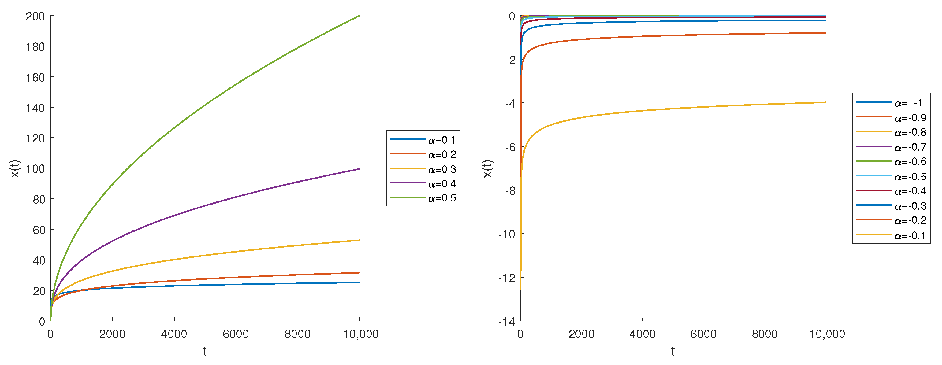
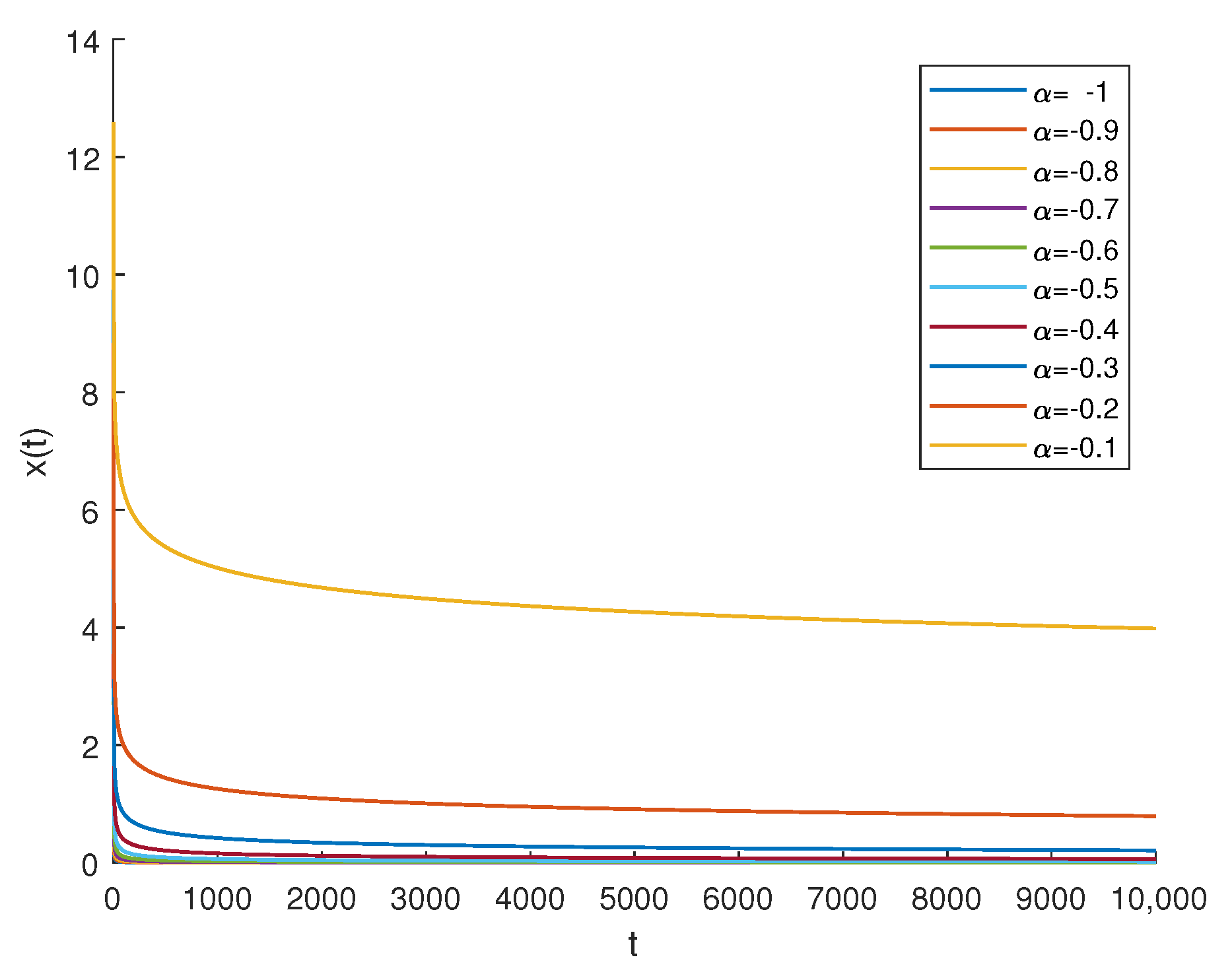
where is an integration constant. For , , and , Equation (4) becomes
and the corresponding trajectories are given in Figure 4 for various values of .
The trajectories in Figure 4 have shapes very similar to that of the densities variations of fixed particles considered above in Figure 2, i.e., with very fast growths for short times, followed by very slow progressions towards a steady state. Figure 5 shows the response of model (3) for various values of with , , and . These responses look like the one of a fractional integrator impulse response.
This model was thus used in a first approach to model the RSA density on the fractals considered in the previous section. An optimization was performed on parameters A and C. Since the power-law behavior only holds for the high coverage regime (long times) of the RSA process, two optimization criteria were used:
In (6) and (7), denotes the last time point in the considered RSA data and denotes the first time value considered for the computation of the criterion.
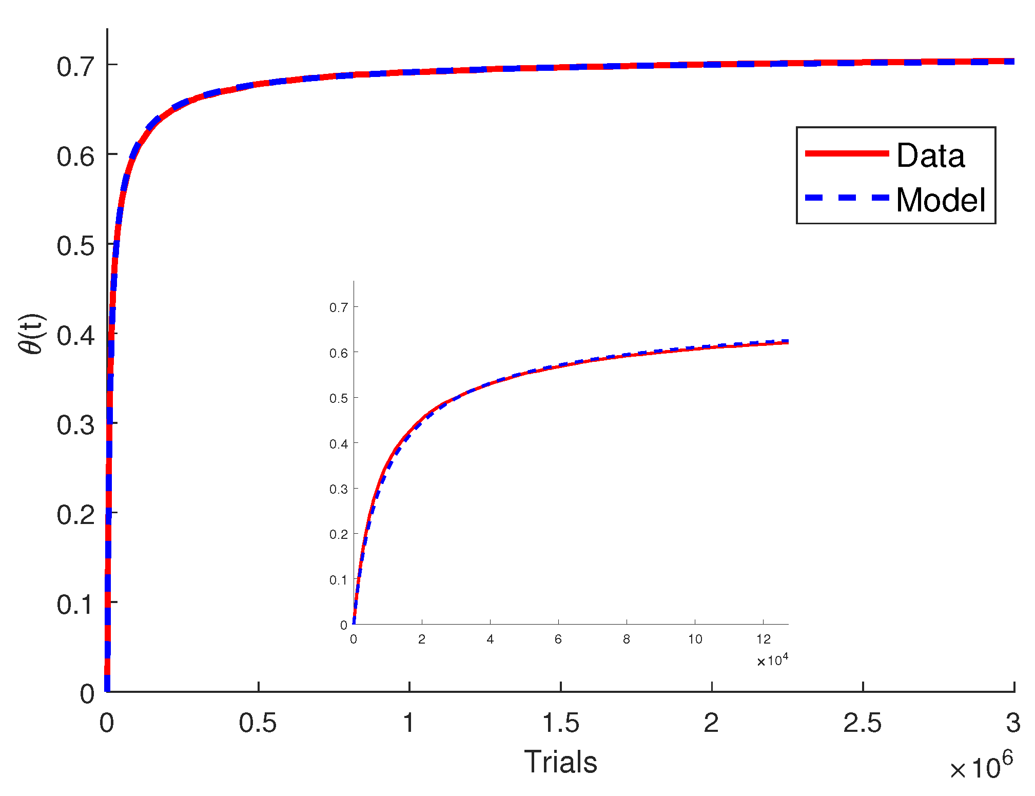
For the Vicsek fractal, parameter was imposed equal to , and the result of this optimization with criterion is given in Figure 6. The following parameters were obtained: and .
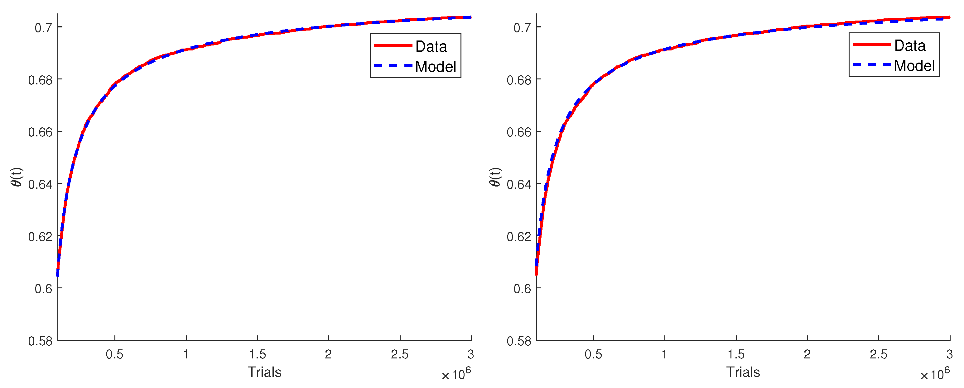
The same optimization was also done using criterion and . A comparison of the RSA density data and of the models obtained with criterion and is shown in Figure 7.
Even if the model parameters were computed using criterion , criterion was computed for the resulting model, and conversely, criterion was computed with the model obtained through the minimization of criterion . The results are reported in Table 2. This table shows that is lower when the parameters are computed with . Model (3) is thus a very good candidate to model fractional dynamics (high coverage times) and achieve a compromise when computed with criterion .
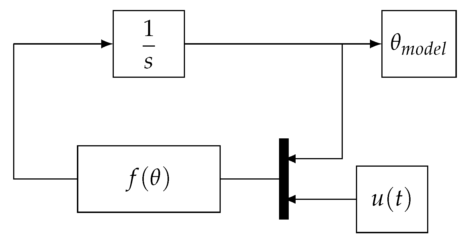
In order to reduce this error, the more general model
is now considered, where f is a polynomial function:
A theoretical justification of this class of model appears in [31]. The proposed model for RSA kinetics of anisotropic particles is based on the available surface function (ASF) concept and is defined by
where is the probability of adding a new particle with orientation to the surface when the coverage is . The function cannot be obtained exactly, but approximations can be computed under the form of series expansions for low and high coverage regimes. These two approximations are then combined to provide an approximate description of the kinetics over the entire coverage range. The following two interpolation formulas are proposed in [31]:
and
Parameters and are then computed to fit the series expansions of the function in (10). An expansion similar to (11) is used in [32,33]:
In [32], parameters , , and are computed as in [31] and to fit insulin adsorption data as [33]. These works, and particularly [31], fully justify the interest of nonlinear models for RSA kinetic modeling and by extension for adsorption kinetics in physical time. However, these models have a constrained form to meet the asymptotic behaviors for low and high surface coverage, which reduces the accuracy of the model outside these coverage regimes.
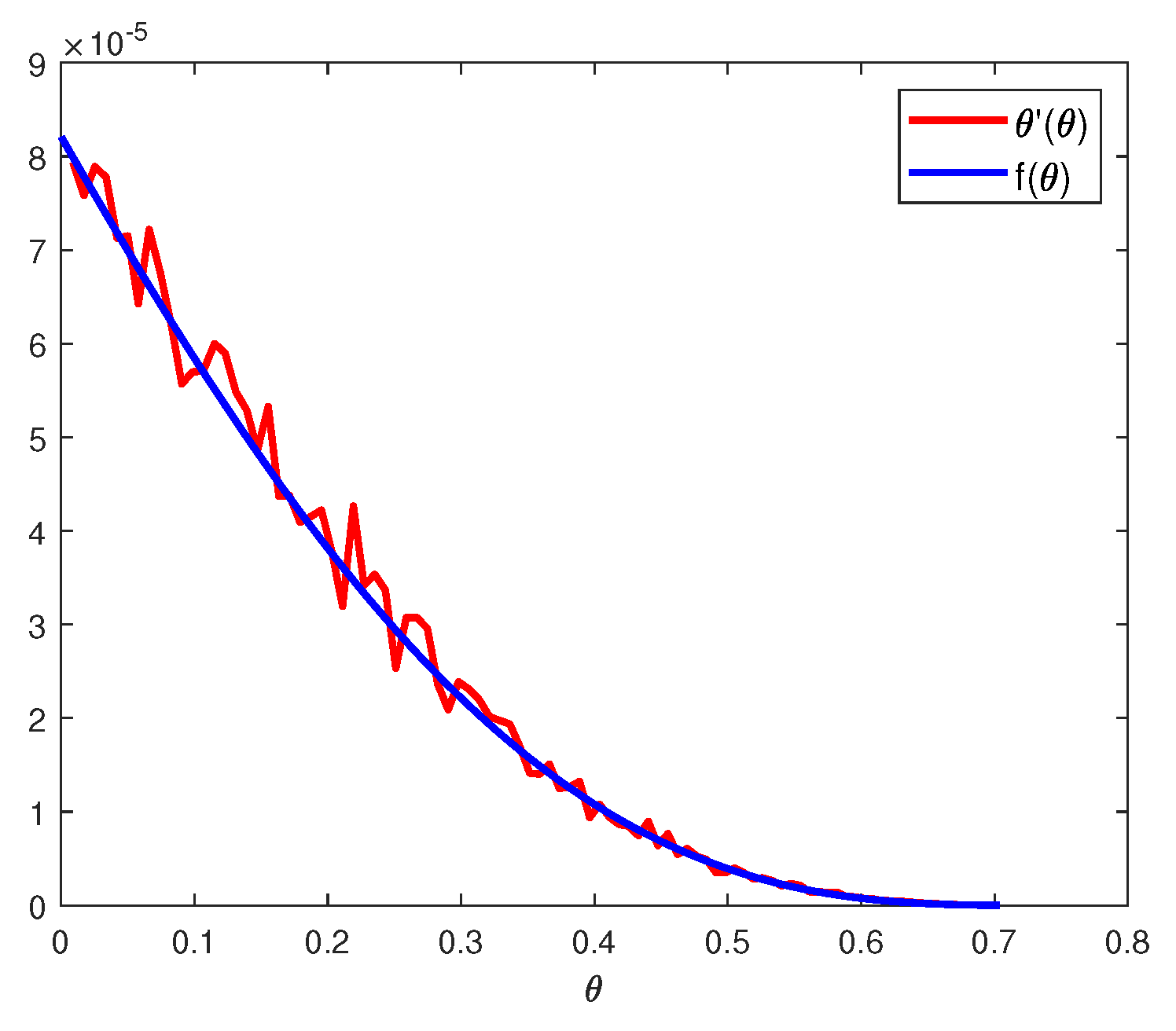
In our approach a more general expansion is considered in the form of model (8) and (9). If , and according to relation (8), this polynomial evaluated in is equal to the derivative of . An optimization was performed on the parameters in order to minimize the quadratic error .
The function is computed numerically from data of Figure 2 and the optimized function f are plotted in Figure 8 as functions of .
The diagram in Figure 9 is an implementation of relation (8) where function f is given by relation (9). Such a diagram is used for simulation of the density of adsorbed disks as a function of time.
The parameters , , , , and given in Table 3 were obtained using the Matlab function fmincon.
3.2. Result for the Other Fractals
The parameters , , , , and given in Table 4 were obtained.
The error with criterion (relation (6)) is
The parameters , , , , and given in Table 5 were obtained.
The error with criterion (relation (6)) is
4. Conclusions
Random sequential adsorption on fractal surfaces is considered in this paper. Numerical simulations confirm that the studied phenomenon exhibits a fractional dynamic linked to the dimension of the fractal surfaces considered. In the literature, fractional behaviors are almost exclusively modeled using fractional models. However, this implicit link between fractional behaviors and fractional models does not result from physical justification. Moreover, as fractional models are doubly infinite dimensional models and thus of infinite memory [34], several limitations are associated with them [35,36]. However, many other classes of model permit to capture fractional behaviors [37,38,39,40]. Here, two driftless control-affine nonlinear models are proposed to capture this dynamic. For the first one, its ability to produce a fractional behavior is proved analytically. It is accurate on the high coverage regime but not on the beginning of the process. For this reason a more complex model but with a limited number of parameters is proposed. Numerical simulations on several fractal surfaces confirmed its efficiency.
Author Contributions
Conceptualisation, V.T., J.S. and C.F.; writing—original draft preparation, V.T., J.S. and C.F.; writing—review and editing, V.T., J.S. and C.F.; All authors have read and agreed to the published version of the manuscript.
Funding
This research received no external funding.
Institutional Review Board Statement
Not applicable.
Informed Consent Statement
Not applicable.
Data Availability Statement
Not applicable.
Acknowledgments
The authors are thankful to Michal Ciesla for fruitful exchanges which helped us progress more rapidly.
Conflicts of Interest
The authors declare no conflict of interest.
References
- Awad, A.M.; Jalab, R.; Benamor, A.; Nasser, M.S.; Ba-Abbad, M.M.; El-Naas, M.; Mohammad, A.W. Adsorption of organic pollutants by nanomaterial-based adsorbents: An overview. J. Mol. Liq. 2020, 301, 112335. [Google Scholar] [CrossRef]
- Ighalo, J.O.; Adeniyi, A.G. Adsorption of pollutants by plant bark derived adsorbents: An empirical review. J. Water Process. Eng. 2020, 35, 101228. [Google Scholar] [CrossRef]
- Bonilla-Petriciolet, A.; Mendoza-Castillo, D.I.; Reynel-Ávila, H.E. Adsorption Processes for Water Treatment and Purification; Springer: Berlin/Heidelberg, Germany, 2017. [Google Scholar]
- Halil, H.; Menini, P.; Aubert, H. Novel microwave gas sensor using dielectric resonator with SnO2 sensitive layer. Procedia Chem. 2009, 1, 935–938. [Google Scholar] [CrossRef]
- Nikolaou, I.; Hallil, H.; Conédéra, V.; Deligeorgis, G.; Dejous, C.; Rebiere, D. Inkjet-printed graphene oxide thin layers on love wave devices for humidity and vapor detection. IEEE Sens. J. 2016, 16, 7620–7627. [Google Scholar] [CrossRef]
- Swendsen, R.H. Dynamics of random sequential adsorption. Phys. Rev. A 1981, 24, 504–508. [Google Scholar] [CrossRef]
- Cieśla, M.; Ziff, R.M. Boundary conditions in random sequential adsorption. J. Stat. Mech. Theory Exp. 2018, 2018, 043302. [Google Scholar] [CrossRef] [Green Version]
- Zhang, G.; Torquato, S. Precise algorithm to generate random sequential addition of hard hyperspheres at saturation. Phys. Rev. E 2013, 88, 053312. [Google Scholar] [CrossRef] [Green Version]
- Feder, J.; Giaever, I. Adsorption of ferritin. J. Colloid Interface Sci. 1980, 78, 144–154. [Google Scholar] [CrossRef]
- Viot, P.; Tarjus, G.; Ricci, S.; Talbot, J. Random sequential adsorption of anisotropic particles. I. Jamming limit and asymptotic behavior. J. Chem. Phys. 1992, 97, 5212–5218. [Google Scholar] [CrossRef] [Green Version]
- Bashiri, H.; Shajari, A. Theoretical Study of Fractal-Like Kinetics of Adsorption. Adsorpt. Sci. Technol. 2014, 32, 623–634. [Google Scholar] [CrossRef]
- Lagergren, S. About the Theory of So-Called Adsorption of Soluble Substances. K. Sven. Vetenskapsakademiens Handl. 1898, 24, 1–39. [Google Scholar]
- Kopelman, R. Fractal Reaction Kinetics. Science 1988, 241, 1620–1626. [Google Scholar] [CrossRef] [PubMed]
- Ho, Y.S.; Mckay, G. The Kinetics of Sorption of Divalent Metal Ions Onto Sphagnum Moss Peat. Water Res. 2000, 34, 735–742. [Google Scholar] [CrossRef]
- Brouers, F.; Sotolongo-Costa, O. Generalized Fractal Kinetics in Complex Systems (Application to Biophysics and Biotechnology). Phys. A Stat. Mech. Its Appl. 2006, 368, 165–175. [Google Scholar] [CrossRef] [Green Version]
- Haerifar, M.; Azizian, S. Fractal-Like Adsorption Kinetics at the Solid/Solution Interface. J. Phys. Chem. C 2012, 116, 13111–13119. [Google Scholar] [CrossRef]
- Tartaglione, V.; Farges, C.; Sabatier, J. Non linear dynamical modeling of adsorption and desorption processes with power-law kinetics: Application to CO2 capture. Phys. Rev. E 2020, 102, 052102. [Google Scholar] [CrossRef]
- Ciesla, M.; Barbasz, J. Random Sequential Adsorption on Fractals. J. Chem. Phys. 2012, 137, 044706. [Google Scholar] [CrossRef] [Green Version]
- Le Mehaute, A.; Crepy, G. Introduction to transfer and motion in fractal media: The geometry of kinetics. Solid State Ion. 1983, 9–10, 17–30. [Google Scholar] [CrossRef]
- Sapoval, B. Universalités et Fractales: Jeux d’enfant ou délits d’initié? Editions Flammarion: Paris, France, 1997. [Google Scholar]
- Krapivsky, P.L.; Redner, S.; Ben-Naim, E. A Kinetic View of Statistical Physics; Cambridge University Press: Cambridge, UK, 2010. [Google Scholar] [CrossRef] [Green Version]
- Qi, H.; Ma, J.; Wong, P.Z. Adsorption isotherms of fractal surfaces. Colloids Surf. A Physicochem. Eng. Asp. 2002, 206, 401–407. [Google Scholar] [CrossRef]
- Watt-Smith, M.; Edler, K.; Rigby, S. An experimental study of gas adsorption on fractal surfaces. Langmuir 2005, 21, 2281–2292. [Google Scholar] [CrossRef]
- Lv, X.; Liang, X.; Xu, P.; Chen, L. A numerical study on oxygen adsorption in porous media of coal rock based on fractal geometry. R. Soc. Open Sci. 2020, 7, 191337. [Google Scholar] [CrossRef] [PubMed] [Green Version]
- Marques, C.; Joanny, J. Adsorption of semi-dilute polymer solutions on fractal colloidal grains. J. Phys. Fr. 1988, 49, 1103–1109. [Google Scholar] [CrossRef] [Green Version]
- Wu, M.K. The Roughness of Aerosol Particles: Surface Fractal Dimension Measured Using Nitrogen Adsorption. Aerosol Sci. Technol. 1996, 25, 392–398. [Google Scholar] [CrossRef]
- Brockett, R.W. Control Theory and Singular Riemannian Geometry. In New Directions in Applied Mathematics: Papers Presented April 25/26, 1980, on the Occasion of the Case Centennial Celebration; Hilton, P.J., Young, G.S., Eds.; Springer: New York, NY, USA, 1982; pp. 11–27. [Google Scholar] [CrossRef]
- Bloch, A.M. Nonholonomic Mechanics and Control; Springer: New York, NY, USA, 2003; pp. 11–27. [Google Scholar]
- M’Closkey, R.; Murray, R. Exponential stabilization of driftless nonlinear control systems using homogeneous feedback. IEEE Trans. Autom. Control 1997, 42, 614–628. [Google Scholar] [CrossRef]
- Wen, J.; Jung, S. Nonlinear model predictive control based on predicted state error convergence. In Proceedings of the IEEE 2004 American Control Conference, Boston, MA, USA, 30 June–2 July 2004; Volume 3, pp. 2227–2232. [Google Scholar] [CrossRef]
- Ricci, S.M.; Talbot, J.; Tarjus, G.; Viot, P. Random sequential adsorption of anisotropic particles. II. Low coverage kinetics. J. Chem. Phys. 1992, 97, 5219–5228. [Google Scholar] [CrossRef] [Green Version]
- Adamczyk, Z.; Barbasz, J.; Cieśla, M. Kinetics of Fibrinogen Adsorption on Hydrophilic Substrates. Langmuir 2010, 26, 11934–11945. [Google Scholar] [CrossRef]
- Ciesla, M.; Barbasz, J. Modeling of interacting dimer adsorption. Surf. Sci. 2013, 612, 24–30. [Google Scholar] [CrossRef] [Green Version]
- Sabatier, J. Fractional Order Models Are Doubly Infinite Dimensional Models and thus of Infinite Memory: Consequences on Initialization and Some Solutions. Symmetry 2021, 13, 1099. [Google Scholar] [CrossRef]
- Sabatier, J.; Farges, C.; Tartaglione, V. Some Alternative Solutions to Fractional Models for Modelling Power Law Type Long Memory Behaviours. Mathematics 2020, 8, 196. [Google Scholar] [CrossRef] [Green Version]
- Sabatier, J. Fractional-Order Derivatives Defined by Continuous Kernels: Are They Really Too Restrictive? Fractal Fract. 2020, 4, 40. [Google Scholar] [CrossRef]
- Sabatier, J. Power Law Type Long Memory Behaviors Modeled with Distributed Time Delay Systems. Fractal Fract. 2020, 4, 1. [Google Scholar] [CrossRef] [Green Version]
- Sabatier, J. Beyond the particular case of circuits with geometrically distributed components for approximation of fractional order models: Application to a new class of model for power law type long memory behaviour modelling. J. Adv. Res. 2020, 25, 243–255. [Google Scholar] [CrossRef] [PubMed]
- Sabatier, J. Non-Singular Kernels for Modelling Power Law Type Long Memory Behaviours and Beyond. Cybern. Syst. 2020, 51, 383–401. [Google Scholar] [CrossRef]
- Sabatier, J. Fractional State Space Description: A Particular Case of the Volterra Equations. Fractal Fract. 2020, 4, 23. [Google Scholar] [CrossRef]
- Liu, K.; Ostadhassan, M.; Jang, H.W.; Zakharova, N.V.; Shokouhimehr, M. Comparison of fractal dimensions from nitrogen adsorption data in shale via different models. R. Soc. Chem. Adv. 2021, 11, 2298–2306. [Google Scholar]
Figure 1.
Vicsek fractal (left), Sierpinski triangle (middle) and Sierpinski carpet (right).

Figure 2.
Densities of adsorbed disks on Vicsek fractal (left), Sierpinski triangle (middle) and Sierpinski carpet (right).
Figure 2.
Densities of adsorbed disks on Vicsek fractal (left), Sierpinski triangle (middle) and Sierpinski carpet (right).

Figure 3.
High regime coverage behavior of RSA on Vicsek fractal (left), Sierpinski triangle (middle) and Sierpinski carpet (right).
Figure 3.
High regime coverage behavior of RSA on Vicsek fractal (left), Sierpinski triangle (middle) and Sierpinski carpet (right).

Figure 4.
Solution with , , and for (left) and (right).

Figure 5.
Solution with , , and for seen as an impulse response.

Figure 6.
Comparison of RSA density data with model (3) response with criterion .
Figure 6.
Comparison of RSA density data with model (3) response with criterion .

Figure 7.
Comparison of RSA density data with model (3) response optimized with criterion (left) and with criterion (right).
Figure 7.
Comparison of RSA density data with model (3) response optimized with criterion (left) and with criterion (right).

Figure 8.
Approximation of the derivative of (red) and function f evaluated in after optimization (blue).
Figure 8.
Approximation of the derivative of (red) and function f evaluated in after optimization (blue).

Figure 9.
Block diagram for simulation of model (8).
Figure 9.
Block diagram for simulation of model (8).

Figure 10.
Comparison between the RSA density data (red) and the model (8) (blue).
Figure 10.
Comparison between the RSA density data (red) and the model (8) (blue).

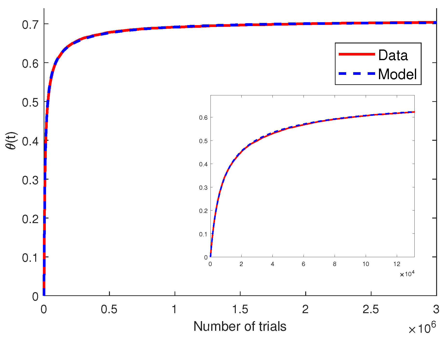
Figure 11.
Comparison between the RSA density data (red) and the model (8) (blue) for Sierpinsky triangle fractal.
Figure 11.
Comparison between the RSA density data (red) and the model (8) (blue) for Sierpinsky triangle fractal.

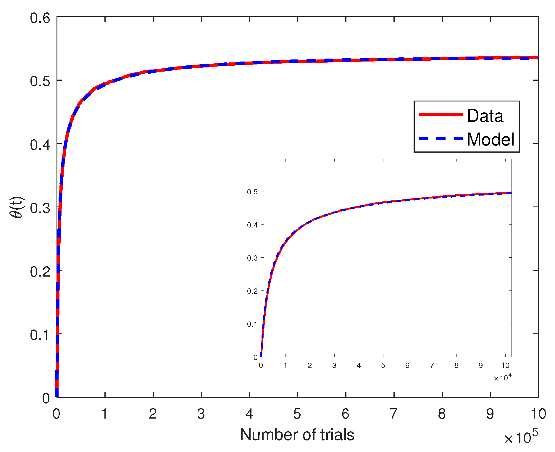
Figure 12.
Comparison between the RSA density data (red) and the model (8) (blue) for Sierpinsky carpet fractal.
Figure 12.
Comparison between the RSA density data (red) and the model (8) (blue) for Sierpinsky carpet fractal.


Table 1.
Final values of the density of adsorbed disks.
| Fractal | Final Value |
|---|---|
| Vicsek | ∼0.68 |
| Sierpinski triangle | ∼0.62 |
| Sierpinski carpet | ∼0.58 |
Table 2.
Error criterion for the three modeling approach.
| Model (3) | Model (3) | Model (8) | |
|---|---|---|---|
| with | with | with | |
Table 3.
Parameters of f in relation (9).
Table 3.
Parameters of f in relation (9).
Table 4.
Parameters of f in relation (9) for the modeling of the Sierpinski triangle.
Table 4.
Parameters of f in relation (9) for the modeling of the Sierpinski triangle.
Table 5.
Parameters of f in relation (9) for the modeling of the Sierpinski carpet.
Table 5.
Parameters of f in relation (9) for the modeling of the Sierpinski carpet.
Publisher’s Note: MDPI stays neutral with regard to jurisdictional claims in published maps and institutional affiliations. |
© 2021 by the authors. Licensee MDPI, Basel, Switzerland. This article is an open access article distributed under the terms and conditions of the Creative Commons Attribution (CC BY) license (https://creativecommons.org/licenses/by/4.0/).
Share and Cite
MDPI and ACS Style
Tartaglione, V.; Sabatier, J.; Farges, C. Adsorption on Fractal Surfaces: A Non Linear Modeling Approach of a Fractional Behavior. Fractal Fract. 2021, 5, 65. https://0-doi-org.brum.beds.ac.uk/10.3390/fractalfract5030065
AMA Style
Tartaglione V, Sabatier J, Farges C. Adsorption on Fractal Surfaces: A Non Linear Modeling Approach of a Fractional Behavior. Fractal and Fractional. 2021; 5(3):65. https://0-doi-org.brum.beds.ac.uk/10.3390/fractalfract5030065
Chicago/Turabian StyleTartaglione, Vincent, Jocelyn Sabatier, and Christophe Farges. 2021. "Adsorption on Fractal Surfaces: A Non Linear Modeling Approach of a Fractional Behavior" Fractal and Fractional 5, no. 3: 65. https://0-doi-org.brum.beds.ac.uk/10.3390/fractalfract5030065