
Existence, Uniqueness, and Eq–Ulam-Type Stability of Fuzzy Fractional Differential Equation


1
Faculty of Mathematics and Computational Science, Xiangtan University, Xiangtan 411105, China
2
Department of Mathematics and Statistics, University of Lahore, Sargodha 40100, Pakistan
3
College of Mathematics and Information Science, Guangxi University, Nanning 530004, China
*
Author to whom correspondence should be addressed.
Fractal Fract. 2021, 5(3), 66; https://0-doi-org.brum.beds.ac.uk/10.3390/fractalfract5030066
Submission received: 26 April 2021
/
Revised: 4 July 2021
/
Accepted: 5 July 2021
/
Published: 11 July 2021
(This article belongs to the Special Issue Fractional Order Systems and Their Applications)
Abstract
:This paper concerns with the existence and uniqueness of the Cauchy problem for a system of fuzzy fractional differential equation with Caputo derivative of order , with initial conditions Moreover, by using direct analytic methods, the –Ulam-type results are also presented. In addition, several examples are given which show the applicability of fuzzy fractional differential equations.
1. Introduction
In real-life phenomena, numerous physical processes are used to present fractional-order sets that may change with space and time. The operations of differentiation and integration of fractional order are authorized by fractional calculus. The fractional order may be taken on imaginary and real values [1,2,3]. The theory of fuzzy sets is continuously drawing the attention of researchers. This is mainly due to its extended adaptability in various fields including mechanics, engineering, electrical, processing signals, thermal system, robotics, control, signal processing, and in several other areas [4,5,6,7,8,9,10]. Therefore, it has been a topic of increasing concern for researchers during the past few years.
Fuzzy fractional differential equations appeared for the first time in 2010 when an idea of the solution was initially proposed by Agarwal et al. [11]. However, the Riemann–Liouville H derivative based on the strongly generalizing Hukuhara differentiability [12,13] was defined by Allahviranloo and Salahshour [14,15]. They worked on solutions to Cauchy problems under this kind of derivative.
In the above, , through using Laplace transforms [13] and Mittag–Leffler functions [12]. By using fractional hyperbolic functions and the properties of these functions, Chehlabi et al. obtain some new results [16]. More latest studies on fuzzy fractional differential equations can be found through references [17,18,19,20,21,22].
In 1940, Ulam promoted the Ulam stability. Lately, Hyers and Rassias used this concept of stability. Since then, in mathematical analysis and differential equations, the Ulam-type stability has had great significance. In fractional differential equations, –Ulam-type stabilities were promoted by Wang in 2014 [23].
In the above equation, and . Shen studied the Ulam stability under the generalization of Hukuhara differentiability of a first-order linear fuzzy differential equation in 2015 [24]. Later, Shen et al. investigated the Ulam stability of a nonlinear fuzzy fractional equation with the help of fixed-point techniques in 2016 [25],
by focusing on the initial condition
where denoted Riemann–Liouville H derivative with respect to order , and .
More results can be observed that are related to Ulam-type stability in [26,27,28]. Motivated by the above-cited papers, we aim to deal with fuzzy fractional differential equations of the form,
with initial conditions
Here, denotes the Caputo derivative of order and .
This paper focuses on facilitating, with as few conditions as possible, to assure the uniqueness and existence of a solution to Cauchy problems (1) and (2). It establishes a link between fuzzy fractional differential equations and the Ulam-type stability, which enhances and generalizes some familiar outputs in the existing literature.
2. Basic Concepts
Assume that denotes the collection of all nonempty convex and compact subsets of and define sums and scalar products in in the usual manner. Let A and B be two nonempty bounded subsets in . The distance between A and B is defined through the Hausdorff metric,
In the above equality, stands for the usual Euclidean norm in . Now it is well known that the metric D turns the space into a complete and separable metric space [26].
Denote
where (1)–(4) stands for the following properties of the function u:
- (1)
- u is normal in the sense that there exists an such that ;
- (2)
- u is fuzzy convex, that is for any and ;
- (3)
- u is an upper semicontinuous function on ;
- (4)
- The set defined by is compact.
For , denote . Now, from (1)–(4), it follows that the q-level set .
Define as the lower branch and as the upper branch of the fuzzy number . The set is known as the q-level set of fuzzy number u, where . The length of q-level set is calculated as diam .
Let and be spaces for all continuous and Lebesgue integrable fuzzy-valued functions on , respectively. Moreover, stands for the complete metric space, where
Remark 1.
On , we can define the subtraction ⊖, called the H difference as follows: makes sense if there exists such that . Then, by definition, .
Let be such that is well defined. Then, its q- is determined by
Through a generalization of the Hausdorff–Pompeiu metric on convex and compact sets, the metric D on can be defined by
Definition 1
([13]). Assume that . The fuzzy Riemann–Liouville integral for a fuzzy-valued function F is defined by
. For we obtain , which is the classical fuzzy integral operator.
Definition 2
It is said that F is Caputo H-differentiable of order at , if there exists an element such that the following fuzzy equalities are valid:
- (i)
- (ii)
- (iii)
- (iv)
Here, we use only the first two cases [23]. These derivatives are trivial because they reduce to crisp elements. Regarding other fuzzy cases, the reader is referred to [23]. Furthermore, regarding this simplicity, a fuzzy-valued function F is called [(i)-GH]-differentiable or [(ii)-GH]-differentiable if it is differentiable according to concept (i) or to (ii) of Definition 2, respectively.
Lemma 2.
Let . Some properties of the functions and are listed below:
- (i)
- Let . Then and ;
- (ii)
- Let and . Then and are positive. If, moreover, , then and ;
- (iii)
- .
Remark 2.
According to the lemma given above, it can be observed that for and . Fractional hyperbolic functions that are generalizations of standard hyperbolic functions can be defined through Mittag–Leffler functions (see, e.g., [16]) as follows:
for . It is noticed that cosh is an even function and that sinh, , is an odd function. For , we write and instead of cosh and sinh respectively. It is not difficult to observe that and (see, e.g., [16]).
Remark 3.
According to the above arguments and Remark 2, we have for any .
Lemma 3.
3. Existence and Uniqueness Results
In this part, existence and uniqueness of solutions to the Cauchy problem in (1) and (2) are discussed. We can start with the lemma given below.
Lemma 4
([16]). When , the [(i)-GH]-differentiable solution to problem (1) is given by
when , the [(ii)-GH]-differentiable solution to problem (1) is given by
when , the [(i)-GH]-differentiable solution to problem (1) is given by
when , the [(ii)-GH]-differentiable solution to problem (1) is given by
when , the [(i)-GH]-differentiable solution to problem (1) is given by
when , the [(ii)-GH]-differentiable solution to problem (1) is given by
Remark 4.
If , then problem (1) reduces to
By applying Lemma 4 and Remark 4 with instead of , it follows that the Cauchy problem in (1) and (2) possesses an integral version. In case and the function is assumed to be [(i)-GH]-differentiable, then the function u satisfies
In case and the function is supposed to be [(ii)-GH]-differentiable, then the function u satisfies
In case and the function is [(i)-GH]-differentiable, then the function u satisfies
In case and the function is [(ii)-GH]-differentiable, then the function u satisfies
We should formulate the basic assumptions before initiating our main work:
- The function is continuous;
- There exists a finite constant such that for all and for all the inequalityis valid and such that is satisfied;
- .
Theorem 1.
Proof.
Let the operator be defined as
Theorem 2.
Let and suppose the conditions are satisfied. Assume that for any ,
is non-decreasing in α,
is non-increasing in α, and for any and
Proof.
Let the operator be defined by
Theorem 3.
Proof.
Let the operator be defined as
. It is not difficult to see that u is a [(i)-GH]-differentiable solution for Cauchy problem (1) and (2) if and only if . Let u and v belong to . From the above Lemmas 1 and 2 and Remarks 2 and 3 we deduce
For and for all , which signifies as
Theorem 4.
Let and suppose that the conditions – are satisfied. Assume that for all the functions
is non-decreasing in α. in addition, the function
are non-increasing in α. Furthermore, assume for all , the function
is non-decreasing in α. In addition, the function
is non-increasing in α. In addition, the function for all
is non-decreasing in α, the expression
is non-increasing in α, and for all and ,
Proof.
Let the operator be defined as
According to conditions – and [21], it is known that is well illustrated on . From the above Lemmas 1, 2, and Remark 2,
for and for all , which means that
4. Stability Results
In various studies, –Ulam-type stability approaches regarding fractional differential equations [23] and Ulam-type stability approaches regarding fuzzy differential equations [24,25] were established. Afterward, Yupin Wang and Shurong Sun worked on –Ulam-type stability concepts regarding fuzzy fractional differential equation where . We offer some new –Ulam-type stability concepts regarding fuzzy fractional differential equation where .
Assume that is a constant and that is a positive continuous function. In addition, suppose that is a continuous function that solves the equation in (1) and consider the following related inequalities:
where .
Definition 3.
Definition 4.
Definition 5.
Definition 6.
Lemma 5.
The function with the property that exists in for all satisfies the inequality (3) if and only if there exists a function such that
(i) for all ,
and the function itself satisfies
(ii) for all .
Proof.
The sufficiency begins obviously, and we will only prove the necessity. From condition , we observe that the function defined by
belongs to and that h(t) belongs to for all . Therefore, it follows that the equation in (ii) is satisfied. Additionally, we have
From the inequality (3), it then follows that , and therefore, (i) is satisfied. This completes the proof of Lemma 5. □
Lemma 6.
Proof.
Now, regarding clarity, the proof can be divided into two cases.
Case 1.
Suppose . Then, we write
Observing that u is a [(i)-GH]-differentiable solution of Equation (6), then Lemma 4 with instead of shows the equality
Now, it follows that
Case 2.
When , we denote
It should be observed that is a [(ii)-GH]-differentiable solution of Equation (6) that obeys the inequality in (3). An application of Lemma 5 then yields
Now, it follows that
Now, the proof is completed. □
Lemma 7.
Let be a [(ii)-GH]-differentiable function that solves the Cauchy equation in (1) and (2) and satisfies the inequality (3) and is such that . Let the condition in be satisfied. Then, for every the function satisfies the integral inequality
when , and
when and . Here, the functions and are defined by
Proof.
Now, regarding clarity, the proof can be divided into two cases.
Case 1.
When , observe that u is a [(ii)-GH]-differentiable solution of Equation (5), then the Lemma 5 with instead of shows the equality
Now, it follows that
Case 2.
Suppose . Then, we denote
Observing that is a [(ii)-GH]-differentiable solution of Equation (5), then Lemma 5 with instead of shows the equality
Now, it follows that
Now, the proof is completed. □
Theorem 5.
Suppose , condition – are satisfied, and the following condition holds ; there exists a positive, increasing, and continuous function ζ such that
Proof.
According to Theorem 1, u is a [(i)-GH]-differentiable solution to Cauchy problem (1) and (2). Let u be a [(i)-GH]-differentiable solution to Equation (1), which satisfies inequality (5) with . From Lemma 6, we obtain
. According to condition , it follows that
By the generalized Gronwall inequality [36], we obtain
Thus, Equation (1) is –Ulam–Hyers–Rassias stable in view of Definition 5. □
Theorem 6.
Proof.
According to Theorem 2, u is a -GH]-differentiable solution to Cauchy problem (1) and (2). Let u be a [(ii)-GH]-differentiable solution to Equation (1), which satisfies inequality (5) with . From Lemma 7, we obtain
. According to condition it follows that
By the generalized Gronwall inequality, we obtain
Thus, Equation (1) is –Ulam–Hyers–Rassias stable in view of Definition 5. □
Theorem 7.
Proof.
According to Theorem 3, u is a [(i)-GH]-differentiable solution to Cauchy problem (1) and (2). Let u be a [(i)-GH]-differentiable solution to Equation (1), which satisfies inequality (5) with . From Lemma 6, we obtain
. According to condition , it follows that
By the generalized Gronwall inequality, we obtain
Thus, Equation (1) is –Ulam–Hyers–Rassias stable in view of Definition 5. □
Theorem 8.
Proof.
According to Theorem 4, set u is a [(ii)-GH]-differentiable solution to Cauchy problem (1) and (2). let u be a [(ii)-GH]-differentiable solution to Equation (1), which satisfies the inequality (5) with . from Lemma 7, we obtain
. According to condition , it follows that
By the generalized Gronwall inequality, we obtain
Thus, Equation (1) is –Ulam–Hyers–Rassias stable in view of Definition 5. Now, the proof is completed. □
Remark 7.
Remark 8.
Condition weakens when we assume . This means that certain theorems in [25] are special cases of Theorem 5 and 6 in the present paper.
5. Examples
In this part, we will show four examples to explain our main results.
Example 1.
Consider the following Cauchy problem in terms of a Fuzzy fractional differential equation
on , with initial conditions
Compared to Equation (1), in the above equations, , , , , and is a symmetric triangular fuzzy number. Hence, with , the condition and are satisfied. It is not difficult to prove that condition is satisfied. Hence, as a consequence of Theorem 1, the Cauchy problem (7) and (8) has a [(i)-GH]-differentiable solution. The numerical solutions with respect to the level are provided by utilizing the Adams–Moultan predictor–corrector method.
Furthermore, for , assume that the [(i)-GH]-differentiable fuzzy-valued function satisfies condition and
Assuming and , this means that condition is satisfied. Hence, Equation (7) is –Ulam–Hyers–Rassias stable with respect to Theorem 5.
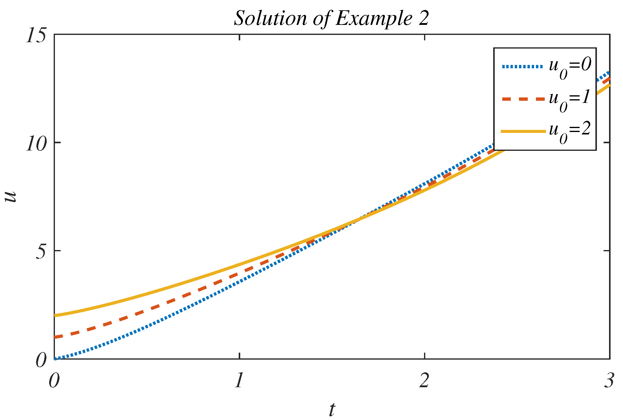
Example 2.
Consider the following Cauchy problem in terms of a Fuzzy fractional differential equation
with initial condition
Compared to Equation (1), in the above equation, , , and is a symmetric triangular fuzzy number.
Hence, with , the condition – are satisfied. It is not difficult to prove that condition is satisfied. Hence, by employing Theorem 2, the Cauchy problem (9)–(10) has a different [(ii)-GH]-differentiable solution. The numerical solution provides with respect to q-level by utilizing the Adams–Moultan predictor–corrector method.
Furthermore, for , assumes that the [(ii)-GH]-differentiable fuzzy-valued function satisfies condition and
Assuming and , this means that condition is satisfied. Hence, Equation (9) is –Ulam–Hyers–Rassias stable with respect to Theorem 6.
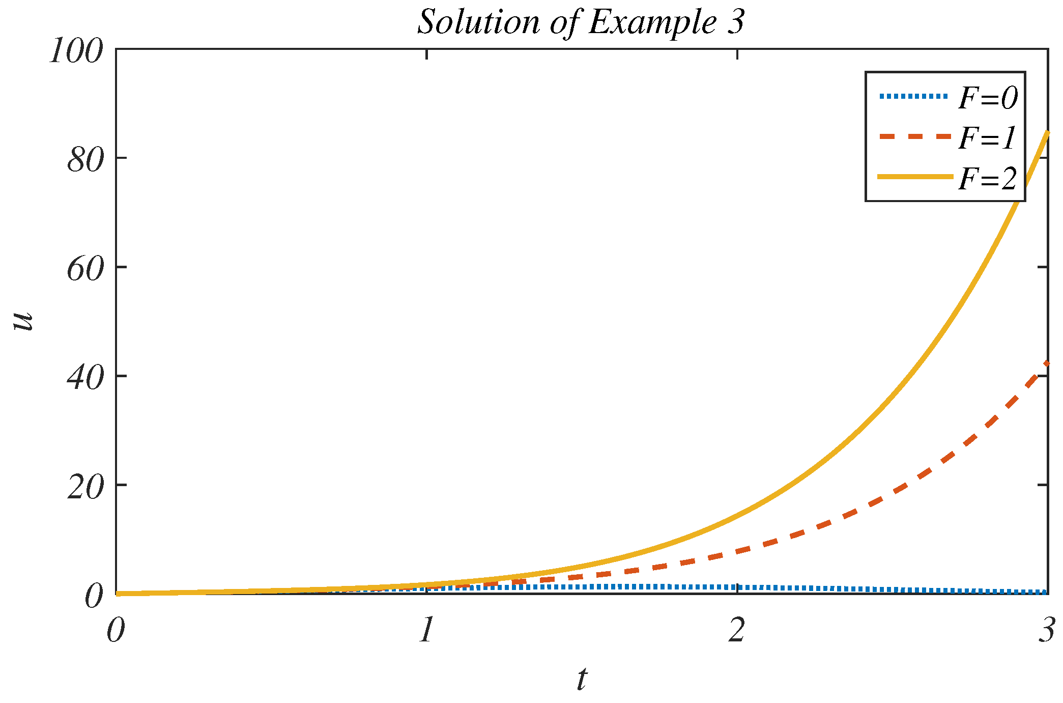
Example 3.
Consider the following Cauchy problem in terms of a Fuzzy fractional differential equation
on , with initial conditions
Compared to equations (1), in the above equation, , , and is a symmetric triangular fuzzy number. Hence, with , it is not difficult to prove that condition and are satisfied. Hence, as a consequence of Theorem 3, the Cauchy problem (11) and (12) has a [(i)-GH]-differentiable solution. The numerical solutions with respect to level are provided by utilizing the Adams–Moultan predictor–corrector method.
Furthermore, for , assume that the [(i)-GH]-differentiable fuzzy-valued function satisfies condition and
Assuming and , this means that condition satisfied. Hence, Equation (11) is –Ulam–Hyers–Rassias stable with respect to Theorem 7.
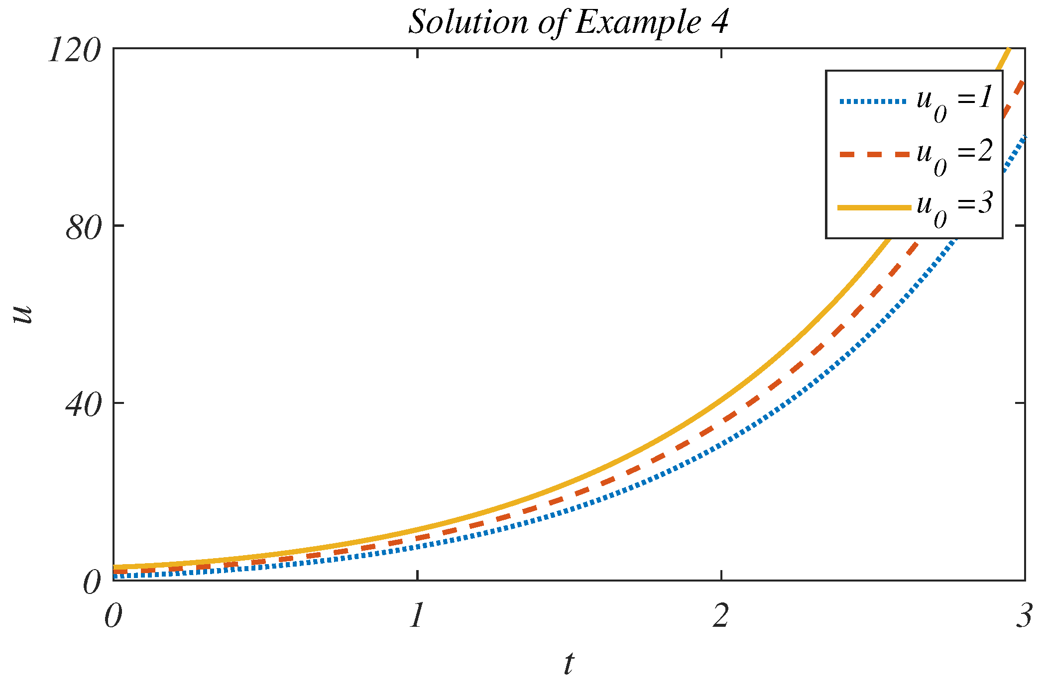
Example 4.
Consider the following Cauchy problem in terms of a Fuzzy fractional differential equation
with initial condition
Compared to Equation (1), in the above equations, , , and is a symmetric triangular fuzzy number.
Hence, with , the condition – are satisfied. Notice and for . It is not difficult to prove that condition – are satisfied. Hence, as a consequence of Theorem 4, the Cauchy problem (13) and (14) has a unique [(ii)-GH]-differentiable solution. The numerical solutions with respect to the level are provided by utilizing the Adams–Moultan predictor–corrector method.
Furthermore, for , assume that the [(ii)-GH]-differentiable fuzzy-valued function satisfies condition and
Assuming and , this means that condition satisfied. Hence, Equation (13) is –Ulam–Hyers–Rassias stable with respect to Theorem 8.
6. Graphical Presentation
We used the Adams–Bashforth–Moulton technique to acquire the numerical solution for this fractional differential equation for graphical representation of the solution of the problem presented in Equations (7), (9), (11) and (13). For simulation, the modified predictor–corrector scheme is used to examine the effect and contribution of the time-delayed factor. A graphical representation of the solution with different variations of the time delay factor, as well as other parameters, is made to check and demonstrate the stability of the model under consideration. We are able to see the Ulam–Hyers stability of varied accuracies and delays from the numerical data. The system will attain Ulam–Hyers stability more quickly with greater accuracy. This is also true when the number of delays increases. Figure 1, Figure 2, Figure 3 and Figure 4 show the stability of the system (7), (9), (11) and (13) for various time delays and fractional derivatives.
7. Conclusions
This paper aims to define the uniqueness and existence of a group of nonlinear fuzzy fractional differential equation of solutions to the Cauchy problem. Moreover, –Ulam-type stability of Equation (1) is observed by applying the inequality technique. We obtain uniqueness and existence results with the help of nonlocal conditions of the Caputo derivative. Moreover, future work may include broadening the idea indicated in this task and familiarizing observability, and generalize other tasks. Ulam-type stability of fuzzy fractional differential equations, similar to crisp situations for approximate solutions, provides a reliable theoretical basis. This a fruitful area with wide research projects, and it can bring about countless applications and theories. We have decided to devote much attention to this area. Furthermore, it is fruitful to investigate stability problems in a classical sense for the fuzzy fractional differential equation.
Author Contributions
A.U.K.N., J.H., R.S. and B.A. contributed equally to the writing of this paper. All authors studied and validated the final document. All authors have read and agreed to the published version of the manuscript.
Funding
The work was of Azmat Ullah Khan Niazi, and supported by post doctoral funding of Xiangtan University, Hunan, China.
Institutional Review Board Statement
Not applicable.
Informed Consent Statement
Not applicable.
Data Availability Statement
All the data is present within the manuscript.
Acknowledgments
The authors would like to express their sincere gratitude to the reviewers and the editors for their careful reviews and constructive recommendations. Jiawei He was supported by the Hunan key Laboratory for Computation and Simulation in Science and Engineering Xiangtan University.
Conflicts of Interest
All authors have no conflict of interest.
References
- Miller, K.S.; Ross, B. An Introduction to the Fractional Calculus and Fractional Differential Equations; Wiley: New York, NY, USA, 1993. [Google Scholar]
- Oldham, K.; Spanier, J. The Fractional Calculus Theory and Applications of Differentiation and Integration to Arbitrary Order; Elsevier: Amsterdam, The Netherlands, 1974. [Google Scholar]
- Samko, S.G.; Kilbas, A.A.; Marichev, O.I. Fractional Integrals and Derivatives (Theory and Applications); Gordon and Breach Science Publishers: Amsterdam, The Netherlands, 1993. [Google Scholar]
- Ahmad, B.; Nieto, J.J. Existence results for a coupled system of nonlinear fractional differential equations with three-point boundary conditions. Comput. Math. Appl. 2009, 58, 1838–1843. [Google Scholar] [CrossRef] [Green Version]
- Ahmad, B.; Ntouyas, S.K.; Agarwal, R.P.; Alsaedi, A. On fractional differential equations and inclusions with nonlocal and average-valued (integral) boundary conditions. Adv. Differ. Equ. 2016, 2016, 80. [Google Scholar] [CrossRef] [Green Version]
- Ding, Z.; Ma, M.; Kandel, A. Existence of the solutions of fuzzy differential equations with parameters. Inf. Sci. 1997, 99, 205–217. [Google Scholar] [CrossRef]
- Kilbas, A.A.; Srivastava, H.M.; Trujillo, J.J. Theory and Applications of Fractional Differential Equations; Elsevier: Amsterdam, The Netherlands, 2006; Volume 204. [Google Scholar]
- Lakshmikantham, V.; Vatsala, A.S. Basic theory of fractional differential equations. Nonlinear Anal. Theory Methods Appl. 2008, 69, 2677–2682. [Google Scholar] [CrossRef]
- Podlubny, I. Fractional Differential Equations: An Introduction to Fractional Derivatives, Fractional Differential Equations, to Methods of Their Solution and Some of Their Applications; Elsevier: Amsterdam, The Netherlands, 1998. [Google Scholar]
- Sakulrang, S.; Moore, E.J.; Sungnul, S.; de Gaetano, A. A fractional differential equation model for continuous glucose monitoring data. Adv. Differ. Equ. 2017, 2017, 150. [Google Scholar] [CrossRef]
- Agarwal, R.; Lakshmikantham, V.; Nieto, J. On the concept of solution for fractional differential equations with uncertainty. Nonlinear Anal. 2010, 72, 2859–2862. [Google Scholar] [CrossRef]
- Allahviranloo, T.; Salahshour, S.; Abbasbandy, S. Explicit solutions of fractional differential equations with uncertainty. Soft Comput. 2012, 16, 297–302. [Google Scholar] [CrossRef]
- Salahshour, S.; Allahviranloo, T.; Abbasbandy, S. Solving fuzzy fractional differential equations by fuzzy Laplace transforms. Commun. Nonlinear Sci. Numer. Simul. 2012, 17, 1372–1381. [Google Scholar] [CrossRef]
- Bede, B.; Gal, S.G. Almost periodic fuzzy-number-valued functions. Fuzzy Sets Syst. 2004, 147, 385–403. [Google Scholar] [CrossRef]
- Bede, B.; Gal, S.G. Generalizations of the differentiability of fuzzy-number-valued functions with applications to fuzzy differential equations. Fuzzy Sets Syst. 2005, 151, 581–599. [Google Scholar] [CrossRef]
- Chehlabi, M.; Allahviranloo, T. Concreted solutions to fuzzy linear fractional differential equations. Appl. Soft Comput. 2016, 44, 108–116. [Google Scholar] [CrossRef]
- Allahviranloo, T.; Armand, A.; Gouyandeh, Z. Fuzzy fractional differential equations under generalized fuzzy Caputo derivative. J. Intell. Fuzzy Syst. 2014, 26, 1481–1490. [Google Scholar] [CrossRef]
- Armand, A.; Allahviranloo, T.; Abbasbandy, S.; Gouyandeh, Z. Fractional relaxation-oscillation differential equations via fuzzy variational iteration method. J. Intell. Fuzzy Syst. 2017, 32, 363–371. [Google Scholar] [CrossRef]
- Wang, Y.; Sun, S.; Han, Z. Existence of solutions to periodic boundary value problems for fuzzy fractional differential equations. Int. J. Dyn. Syst. Differ. Equ. 2017, 7, 195–216. [Google Scholar] [CrossRef]
- Agarwal, R.P.; Baleanu, D.; Nieto, J.J.; Torres, D.F.; Zhou, Y. A survey on fuzzy fractional differential and optimal control nonlocal evolution equations. J. Comput. Appl. Math. 2018, 339, 3–29. [Google Scholar] [CrossRef] [Green Version]
- Huang, L.L.; Baleanu, D.; Mo, Z.W.; Wu, G.C. Fractional discrete-time diffusion equation with uncertainty: Applications of fuzzy discrete fractional calculus. Phys. A Stat. Mech. Its Appl. 2018, 508, 166–175. [Google Scholar] [CrossRef]
- Wang, Y.; Sun, S.; Han, Z. On fuzzy fractional Schrödinger equations under Caputo’s H-differentiability. J. Intell. Fuzzy Syst. 2018, 34, 3929–3940. [Google Scholar] [CrossRef]
- Wang, J.; Li, X. Eα-Ulam type stability of fractional order ordinary differential equations. J. Appl. Math. Comput. 2014, 45, 449–459. [Google Scholar] [CrossRef]
- Shen, Y. On the Ulam stability of first order linear fuzzy differential equations under generalized differentiability. Fuzzy Sets Syst. 2015, 280, 27–57. [Google Scholar] [CrossRef]
- Wang, Y.; Sun, S. Existence, uniqueness and Eq-Ulam type stability of fuzzy fractional differential equations with parameters. J. Intell. Fuzzy Syst. 2019, 36, 5533–5545. [Google Scholar] [CrossRef]
- Shen, Y. Hyers-Ulam-Rassias stability of first order linear partial fuzzy differential equations under generalized differentiability. Adv. Differ. Equ. 2015, 2015, 351. [Google Scholar] [CrossRef] [Green Version]
- Wang, C.; Xu, T.Z. Hyers-Ulam stability of fractional linear differential equations involving Caputo fractional derivatives. Appl. Math. 2015, 60, 383–393. [Google Scholar] [CrossRef] [Green Version]
- Brzdęk, J.; Eghbali, N. On approximate solutions of some delayed fractional differential equations. Appl. Math. Lett. 2016, 54, 31–35. [Google Scholar] [CrossRef]
- Lakshmikantham, V.; Mohapatra, R.N. Theory of Fuzzy Differential Equations and Inclusions; CRC Press: Boca Raton, FL, USA, 2004. [Google Scholar]
- Lakshmikantham, V.; Bhaskar, T.G.; Devi, J.V. Theory of Set Differential Equations in Metric Spaces; Cambridge Scientific Publishers: Cambridge, UK, 2006. [Google Scholar]
- Gorenflo, R.; Kilbas, A.A.; Mainardi, F.; Rogosin, S.V. Mittag-Leffler Functions, Related Topics and Applications; Springer: Berlin, Germany, 2014; Volume 2. [Google Scholar]
- Wang, J.; Feckan, M.; Zhou, Y. Presentation of solutions of impulsive fractional Langevin equations and existence results. Eur. Phys. J. Spec. Top. 2013, 222, 1857–1874. [Google Scholar] [CrossRef]
- Peng, S.; Wang, J. Cauchy problem for nonlinear fractional differential equations with positive constant coefficient. J. Appl. Math. Comput. 2016, 51, 341–351. [Google Scholar] [CrossRef]
- Melliani, S.; El Allaoui, A.; Chadli, L.S. Relation between fuzzy semigroups and fuzzy dynamical systems. Nonlinear Dyn. Syst. Theory 2017, 17, 60–69. [Google Scholar]
- Bede, B.; Stefanini, L. Generalized differentiability of fuzzy-valued functions. Fuzzy Sets Syst. 2013, 230, 119–141. [Google Scholar] [CrossRef] [Green Version]
- Ye, H.; Gao, J.; Ding, Y. A generalized Gronwall inequality and its application to a fractional differential equation. J. Math. Anal. Appl. 2007, 328, 1075–1081. [Google Scholar] [CrossRef] [Green Version]


Publisher’s Note: MDPI stays neutral with regard to jurisdictional claims in published maps and institutional affiliations. |
© 2021 by the authors. Licensee MDPI, Basel, Switzerland. This article is an open access article distributed under the terms and conditions of the Creative Commons Attribution (CC BY) license (https://creativecommons.org/licenses/by/4.0/).
Share and Cite
MDPI and ACS Style
Niazi, A.U.K.; He, J.; Shafqat, R.; Ahmed, B. Existence, Uniqueness, and Eq–Ulam-Type Stability of Fuzzy Fractional Differential Equation. Fractal Fract. 2021, 5, 66. https://0-doi-org.brum.beds.ac.uk/10.3390/fractalfract5030066
AMA Style
Niazi AUK, He J, Shafqat R, Ahmed B. Existence, Uniqueness, and Eq–Ulam-Type Stability of Fuzzy Fractional Differential Equation. Fractal and Fractional. 2021; 5(3):66. https://0-doi-org.brum.beds.ac.uk/10.3390/fractalfract5030066
Chicago/Turabian StyleNiazi, Azmat Ullah Khan, Jiawei He, Ramsha Shafqat, and Bilal Ahmed. 2021. "Existence, Uniqueness, and Eq–Ulam-Type Stability of Fuzzy Fractional Differential Equation" Fractal and Fractional 5, no. 3: 66. https://0-doi-org.brum.beds.ac.uk/10.3390/fractalfract5030066