Article

Solving a System of Fractional-Order Volterra-Fredholm Integro-Differential Equations with Weakly Singular Kernels via the Second Chebyshev Wavelets Method

1
Department of Mathematics, Faculty of Mathematics, Statistics and Computer Sciences, Semnan University, P.O. Box 35195-363, Semnan 35131-19111, Iran
2
Department of Electrical Engineering, University of Bojnord, P.O. Box 94531-1339, Bojnord 94531-55111, Iran
*
Authors to whom correspondence should be addressed.
Submission received: 1 April 2021 / Revised: 17 June 2021 / Accepted: 11 July 2021 / Published: 14 July 2021
(This article belongs to the Special Issue Fractional Calculus and Special Functions with Applications)

Abstract

:
In this paper, by means of the second Chebyshev wavelet and its operational matrix, we solve a system of fractional-order Volterra–Fredholm integro-differential equations with weakly singular kernels. We estimate the functions by using the wavelet basis and then obtain the approximate solutions from the algebraic system corresponding to the main system. Moreover, the implementation of our scheme is presented, and the error bounds of approximations are analyzed. Finally, we evaluate the efficiency of the method through a numerical example.

1. Introduction

Fractional calculus has been the interest of many scientists and engineers [1,2,3]. Many engineering and science phenomena, such as the heat conduction problem, radiative equilibrium, elasticity and fracture mechanics [4], viscoelastic deformation, viscoelasticity, viscous fluid [5], continuous population [6] and so forth, are modeled using the fractional integro-differential equations with a weakly singular kernel, fractional differential equations, fractional integral equations and system of nonlinear Volterra integro-differential equations. Many applied problems are transformed into the system of fractional differential and integral equations by mathematical modeling [7,8,9,10]. Consequently, it is essential to obtain the approximate solution of a system of integro-differential equations by numerical methods.
In this paper, we solve a system of fractional-order Volterra–Fredholm integro-differential equations with weakly singular kernels in the following form:
D α 1 y 1 ( t ) = λ 1 0 t y 1 ( s ) ( t s ) β 1 d s + λ 2 0 1 k 1 ( t , s ) y 2 ( s ) d s + f 1 ( t ) , D α 2 y 2 ( t ) = λ 3 0 t y 1 ( s ) ( t s ) β 2 d s + λ 4 0 1 k 2 ( t , s ) y 2 ( s ) d s + f 2 ( t ) , y 1 ( 0 ) = a 1 , y 2 ( 0 ) = a 2 ,
where y 1 ( t ) , y 2 ( t ) are unknown functions, the functions f 1 ( t ) , f 2 ( t ) , k 1 ( t , s ) , and k 2 ( t , s ) are known, and λ 1 , λ 2 , λ 3 , λ 4 , a 1 , a 2 are real constants, where 0 < α 1 , α 2 , β 1 , β 2 < 1 and D α 1 , D α 2 denote the Caputo fractional-order derivatives. Furthermore, 1 ( t s ) β 1 and 1 ( t s ) β 2 are the weakly singular kernels of the system of fractional-order Volterra–Fredholm integro-differential equations.
In recent years, researchers have proposed different methods for solving the system of differential equations. In 2015, Sahu and Ray [11] developed a numerical method based on the Legendre hybrid block pulse function to approximate the solution of nonlinear systems of Fredholm-Manhattan integral equations. In the same year, they presented another scheme to solve a system of nonlinear Volterra integro-differential equations using Legendre wavelets [6]. Yüzbasi [12] solved the system of linear Fredholm–Volterra integro-differential equations, which includes the derivatives of unknown functions in integral parts using the Bessel collocation method. In 2016, Deif and Grace [13] developed a new iterative method to approximate the solution of a system of linear fractional differential integral equations. In 2019, Xie and Yi [14] developed a numerical method for solving a nonlinear system of fractional-order Volterra–Fredholm integro-differential equations based on block-pulse functions. In 2020, Saemi et al. [15] developed a solution for the system of fractional-order Volterra–Fredholm integro-differential equations based on Müntz–Legendre wavelets.
Wavelets are one of the most important tools used in various fields such as quantum mechanics, signal processing, image processing, time-frequency analysis and data compression [16]. One of the methods that have been considered in recent years to solve various ordinary and fractional-order equations is the use of wavelets [17,18,19]. Wavelets provide a detailed accurate representation of different types of functions and operators, and their relationship with numerical algorithms [20,21]. The second Chebyshev wavelet is one of the wavelets, which has gained attention in solving many problems and is applicable for solving various types of Volterra integral equations with a weakly singular kernel [17], fractional-order nonlinear Fredholm integro-differential equations [20], fractional-order differential equations [22], a system of linear differential equations [23], fractional-order integro-differential equations with a weakly singular kernel [5], and Abel’s integral equations [16]. Approximation of equations using the second Chebyshev wavelets has been considered by many researchers, such as Zhu and Wang [17,24], Zhou and Xu [21], Wang and Fan [22], Tavassoli Kajani et al. [25], Zhou et al. [26], Yi et al. [27], Lal and Sharma [16], and Manchanda and Rani [23].
In this paper, we apply the second Chebyshev wavelets method to solve the system of fractional-order Volterra–Fredholm integro-differential equations with a weakly singular kernel. In fact, the main purpose of this study is solving the system of equations with singularity. The second Chebyshev wavelets method converts the system of fractional-order Volterra–Fredholm integro-differential equations with a weakly singular kernel to a system of algebraic equations, which can be solved using the conventional linear methods.

2. Preliminaries

In this section, we introduce fractional-order operators, block-pulse functions and explain their features.
Definition 1.
The Riemann–Liouville fractional-order integral operator of order α is given by [17,27]:
I α f ( t ) = 1 Γ ( α ) a t ( t τ ) α 1 f ( τ ) d τ , α > 0 ,
where α ( m 1 , m ] , m N .
The properties of this operator are as follows:
  • I a α I a β f = I a α + β f ,
  • I a α I a β f = I a β I a α f ,
  • I a α t c = Γ ( c + 1 ) Γ ( c + α + 1 ) t c + α .
Definition 2.
The Caputo fractional derivative operator of order α for a function f is given by [17,18,27]:
D α f ( t ) = 1 Γ ( n α ) a t f ( n ) ( τ ) ( t τ ) α n + 1 d τ , α ( n 1 , n ] ,
where n N , and Γ ( . ) is the Gamma function.
The properties between the Caputo fractional-order derivative operator and the Riemann–Liouville fractional-order integral operator is given by the following expressions [17,18,24]:
  • D α I α f ( t ) = f ( t ) ,
  • I α D α f ( t ) = f ( t ) k = 0 m 1 f ( k ) ( 0 ) k ! t k .
Definition 3.
The set of block pulse function on [ 0 , 1 ) is defined as:
b i ( t ) = 1 , i 1 m t < i m 0 , otherwise
where i = 1 , 2 , , m . Furthermore, the vector of block pulse functions is obtained as follows:
B m ( t ) = [ b 1 ( t ) , b 2 ( t ) , . . . , b m ( t ) ] T ,
and the important properties of these functions are as follows:
  • b i ( t ) b j ( t ) = b i ( t ) , i = j , 0 , i j ,
  • 0 1 b i ( t ) b j ( t ) d t = 1 m , i = j , 0 , i j .
Lemma 1.
The block pulse function operational matrix of fractional-order integration F α is obtained by:
I α ( B m ( t ) ) F α B m ( t ) ,
where
F α = 1 m α 1 Γ ( α + 2 ) 1 ξ 1 ξ 2 ξ 3 ξ m 1 0 1 ξ 1 ξ 2 ξ m 2 0 0 1 ξ 1 ξ m 3 0 0 0 1 ξ 1 0 0 0 0 1 ,
and ξ k = ( k + 1 ) α + 1 2 k α + 1 + ( k 1 ) α + 1 , k = 1 , 2 , , m 1 .
For example with α = 0.5 and m = 6 :
F 0.5 = 0.3071 0.2544 0.1656 0.1339 0.1156 0.1033 0 0.3071 0.2544 0.1656 0.1339 0.1156 0 0 0.3071 0.2544 0.1656 0.1339 0 0 0 0.3071 0.2544 0.1656 0 0 0 0 0.3071 0.2544 0 0 0 0 0 0.3071 .

3. The Second Chebyshev Wavelets and Function Approximation

In this section, we introduce the second Chebyshev wavelet and then use this basis to provide an approximation of functions.

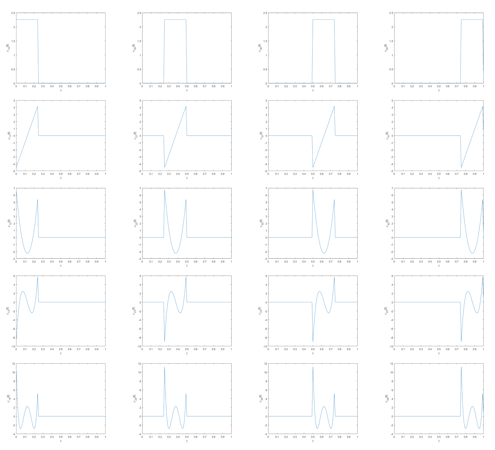
3.1. The Second Chebyshev Wavelets and Their Properties

In this part, we introduce the second Chebyshev wavelet and its features.
Definition 4.
The second Chebyshev wavelet on the interval [ 0 , 1 ) is defined as [16,23,27]:
ψ n m ( t ) = 2 k 2 2 π U m ( 2 k t 2 n + 1 ) , n 1 2 k 1 t < n 2 k 1 , 0 , otherwise ,
where n = 1 , 2 , , 2 k 1 , m = 0 , 1 , , M 1 , and k , M N . The coefficient 2 π is for orthonormality, and U m ( t ) is the Chebyshev polynomial of the second kind with degree m, which is as follows:
U 0 ( t ) = 1 , U 1 ( t ) = 2 t , U m + 1 ( t ) = 2 t U m ( t ) U m 1 ( t ) .
Furthermore, the weight function of the second kind Chebyshev polynomials is ω ( t ) = 1 t 2 , and with transmission and dilation, first we obtain ω ^ ( t ) = ω ( 2 t 1 ) , and then we get ω n ( t ) = ω ( 2 k t 2 n + 1 ) as the weight function of the second Chebyshev wavelets basis.
For example, with k = 2 and M = 3 , we have n = 1 , 2 , m = 0 , 1 , 2 , and for 0 t < 0.5 ,
ψ 10 ( t ) = 2 2 π U 0 ( 4 t 1 ) = 2 2 π , ψ 11 ( t ) = 2 2 π U 1 ( 4 t 1 ) = 2 2 π ( 8 t 2 ) , ψ 12 ( t ) = 2 2 π U 2 ( 4 t 1 ) = 2 2 π ( 64 t 2 32 t + 3 ) ,
and also for 0.5 t < 1 ,
ψ 20 ( t ) = 2 2 π U 0 ( 4 t 3 ) = 2 2 π , ψ 21 ( t ) = 2 2 π U 1 ( 4 t 3 ) = 2 2 π ( 8 t 6 , ) ψ 22 ( t ) = 2 2 π U 2 ( 4 t 3 ) = 2 2 π ( 64 t 2 96 t + 35 ) .
The second Chebyshev wavelets have an orthonormal basis of L 2 [ 0 , 1 ) , i.e.,
< ψ n m ( t ) , ψ n m ( t ) > ω n = 0 1 ψ n m ( t ) ψ n m ( t ) ω n ( t ) d t = 1 , m = m , n = n , 0 , o . w . ,
where < . , . > ω n denotes the inner product. The second Chebyshev wavelet has compact support [ n 1 2 k 1 , n 2 k 1 ] , n = 1 , , 2 k 1 . The Chebyshev wavelet charts for k = 3 and M = 4 are shown in Figure 1.
According to the second Chebyshev wavelet, the vector of this wavelet is given by [16,27]:
Ψ ( t ) = [ ψ 10 ( t ) , ψ 11 ( t ) , , ψ 1 ( M 1 ) ( t ) , ψ 20 ( t ) , ψ 21 ( t ) , , ψ 2 ( M 1 ) ( t ) , , ψ 2 k 1 0 ( t ) , ψ 2 k 1 1 ( t ) , , ψ 2 k 1 ( M 1 ) ( t ) ] T .
In other words, for 0 t < 0.5 :
Ψ ( t ) = 2 2 π 2 2 π ( 8 t 2 ) 2 2 π ( 64 t 2 32 t + 3 ) 0 0 0 ,
and for 0.5 t < 1 :
Ψ ( t ) = 0 0 0 2 2 π 2 2 π ( 8 t 6 ) 2 2 π ( 64 t 2 96 t + 35 ) .
Moreover, for the collocation points [24]
t i = 2 i 1 2 m , i = 1 , 2 , , m ,
with m = 2 k 1 M , the second Chebyshev wavelets matrix is obtained as follows [24,25]:
Φ m × m = [ Ψ ( 1 2 m ) , Ψ ( 3 2 m ) , , Ψ ( 2 m 1 2 m ) ] .
For k = 2 and M = 3 , i.e.,
Φ = 1.59576 1.59576 1.59576 0 0 0 2.12769 0 2.12769 0 0 0 1.24115 1.59576 1.24115 0 0 0 0 0 0 1.59576 1.59576 1.59576 0 0 0 2.12769 0 2.12769 0 0 0 1.24115 1.59576 1.24115 .
There is a relationship between the second Chebyshev wavelet and the block pulse function:
Ψ ( t ) = Φ B m ( t ) .
If I α is the fractional-order integration operator of the second Chebyshev wavelets, one can achieve [17,24]:
I α Ψ ( t ) P α Ψ ( t ) , with P α = Φ F α Φ 1 ,
where P α is named as the operational matrix of fractional-order integration of the second Chebyshev wavelet. For example,
P 0.5 = 0.5365 0.1575 0.0249 0.4366 0.0754 0.0214 0.0191 0.0449 0.0858 0.1287 0.2242 0.2105 0.0512 0.0470 0.1604 0.0948 0.0253 0.0100 0 0 0 0.5365 0.1575 0.0249 0 0 0 0.2105 0.2242 0.1287 0 0 0 0.0512 0.0470 0.1604 .

3.2. Function Approximation

Using the second Chebyshev wavelet, each function in L 2 can be approximated using the following lemma.
Lemma 2.
Any function f L 2 ( [ 0 , 1 ] ) can be expanded into the second Chebyshev wavelet as [16,27,28]:
f ( t ) = n = 1 m Z c n m ψ n m ( t ) ,
where
c n m = f ( t ) , ψ n m ( t ) ω n = 0 1 ψ n m ( t ) f ( t ) ω n ( t ) d t .
If Equation (6) is truncated, then with Equation (3)
f ( t ) n = 1 2 k 1 m = 0 M 1 c n m ψ n m ( t ) = C T Ψ ( t ) .
Remark 1.
Let X L 2 ( [ 0 , 1 ] ) , so
I α X ( t ) I α C T Ψ ( t ) = C T I α Ψ ( t ) = C T P α Ψ ( t ) .

4. Method Analysis

For solving the system (1), without reducing the generality of the equations under consideration, we assume that the initial conditions are zero, and we approximate D α y i ( t ) , f i ( t ) , and k i ( t , s ) for i = 1 , 2 in terms of the second Chebyshev wavelet as follows:
D α i y i ( t ) C i T Ψ ( t ) , f i ( t ) F i T Ψ ( t ) , k i ( t , s ) Ψ T ( t ) K i Ψ ( s ) .
From Equations (2), (7) and (8), we obtain
y i ( t ) = I α i D α i y i ( t ) C i T P α i Ψ ( t ) .
Thus,
0 t y i ( s ) ( t s ) β i d s = C i T P α i 0 t Ψ ( s ) ( t s ) β i d s = C i T P α i Γ ( 1 β i ) I 1 β i Ψ ( t ) = Γ ( 1 β i ) C i T P α i P 1 β i Ψ ( t ) ,
and from Equation (8) and 0 1 Ψ ( s ) Ψ ( s ) T d s = D , we have
0 1 k i ( t , s ) y i ( s ) d s = 0 1 Ψ T ( t ) K i Ψ ( s ) Ψ ( s ) T P α i T C i d s = Ψ T ( t ) K i 0 1 Ψ ( s ) Ψ ( s ) T d s P α i T C i = Ψ T ( t ) K i D P α i T C i = C i T P α i D T K i T Ψ ( t ) .
By substituting Equations (8)–(11) into (1), we get
C 1 T Ψ ( t ) = λ 1 Γ ( 1 β 1 ) C 1 T P α 1 P 1 β 1 Ψ ( t ) + λ 2 C 2 T P α 2 D T K 1 T Ψ ( t ) + F 1 T Ψ ( t ) , C 2 T Ψ ( t ) = λ 3 Γ ( 1 β 2 ) C 1 T P α 1 P 1 β 2 Ψ ( t ) + λ 4 C 2 T P α 2 D T K 2 T Ψ ( t ) + F 2 T Ψ ( t ) ,
and we obtain
C 1 T = λ 1 Γ ( 1 β 1 ) C 1 T P α 1 P 1 β 1 + λ 2 C 2 T P α 2 D T K 1 T + F 1 T , C 2 T = λ 3 Γ ( 1 β 2 ) C 1 T P α 1 P 1 β 2 + λ 4 C 2 T P α 2 D T K 2 T + F 2 T .
By solving system (13), one can get C 1 and C 2 . Then substituting them into (9), the unknown solutions can be obtained.

5. Error Analysis

In this section, we present an error estimation for the system of Equation (1).
Theorem 1.
Let y ^ 1 ( t ) and y ^ 2 ( t ) be the approximations of y 1 ( t ) and y 2 ( t ) , obtained by the second Chebyshev wavelets basis (6), as the solutions of system (1) with 0 < β 1 , β 2 < 1 / 2 . Assume also that there is a pair of constants k 1 and k 2 such that
k i ( t , s ) 2 = < k i ( t , s ) , k i ( t , s ) > 1 2 = 0 1 0 1 | k i ( t , s ) | 2 d t d s 1 2 k i , i = 1 , 2 .
If
| λ 1 | < Γ ( 2 + α 1 ) 1 2 β 1 ,
k 2 | λ 4 | < Γ ( 1 + α 2 ) ,
| λ 1 | ( 1 + α 1 ) 1 2 β 1 + k 1 | λ 2 λ 3 | ( 1 + α 2 ) 1 2 β 2 Γ ( 1 + α 2 ) k 2 | λ 4 | < Γ ( 1 + α 1 ) ,
and
k 1 | λ 2 λ 3 | ( 1 + α 1 ) 1 2 β 1 ( 1 + α 2 ) 1 2 β 2 Γ ( 2 + α 1 ) 1 2 β 1 | λ 1 | + k 2 | λ 4 | < Γ ( 1 + α 2 ) ,
then the approximate solutions of system (1) converge to the exact solutions with respect to L 2 norm.
Proof. 
Compute, by the assumptions,
y 1 y ^ 1 2 = I α 1 λ 1 0 t y 1 ( s ) y ^ 1 ( s ) ( t s ) β 1 d s + λ 2 0 1 k 1 ( t , s ) ( y 2 ( s ) y ^ 2 ( s ) ) d s 2 ,
and
y 2 y ^ 2 2 = I α 2 λ 3 0 t y 1 ( s ) y ^ 1 ( s ) ( t s ) β 2 d s + λ 4 0 1 k 2 ( t , s ) ( y 2 ( s ) y ^ 2 ( s ) ) d s 2 .
Using the triangular inequality, we get
y 1 y ^ 1 2 I α 1 | λ 1 | 0 t ( t s ) β 1 2 y 1 y ^ 1 2 d s + | λ 2 | 0 1 k 1 ( t , s ) 2 y 2 y ^ 2 2 d s ,
and
y 2 y ^ 2 2 I α 2 | λ 3 | 0 t ( t s ) β 2 2 y 1 y ^ 1 2 d s + | λ 4 | 0 1 k 2 ( t , s ) 2 y 2 y ^ 2 2 d s .
Furthermore, for 0 < β 1 , β 2 < 1 / 2 and 0 t 1 , we have
( t s ) β 1 2 = 0 1 1 ( t s ) 2 β 1 d s 1 2 1 1 2 β 1 , ( t s ) β 2 2 = 0 1 1 ( t s ) 2 β 2 d s 1 2 1 1 2 β 2 ,
and as a result, we obtain
y 1 y ^ 1 2 | λ 1 | Γ ( 2 + α 1 ) 1 2 β 1 y 1 y ^ 1 2 + k 1 | λ 2 | Γ ( 1 + α 1 ) y 2 y ^ 2 2 ,
and
y 2 y ^ 2 2 | λ 3 | Γ ( 2 + α 2 ) 1 2 β 2 y 1 y ^ 1 2 + k 2 | λ 4 | Γ ( 1 + α 2 ) y 2 y ^ 2 2 .
Now, we denote
e i ( t ) = y i ( t ) y ^ i ( t ) 2 , i = 1 , 2 ,
so,
e 1 ( t ) | λ 1 | Γ ( 2 + α 1 ) 1 2 β 1 e 1 ( t ) + k 1 | λ 2 | Γ ( 1 + α 1 ) e 2 ( t ) ,
and consequently by the assumption | λ 1 | < Γ ( 2 + α 1 ) 1 2 β 1 , one can conclude
e 1 ( t ) k 1 | λ 2 | Γ ( 1 + α 1 ) 1 | λ 1 | Γ ( 2 + α 1 ) 1 2 β 1 e 2 ( t ) .
We have similar relations for the second approximation, i.e.,
e 2 ( t ) | λ 3 | Γ ( 2 + α 2 ) 1 2 β 2 e 1 ( t ) + k 2 | λ 4 | Γ ( 1 + α 2 ) e 2 ( t ) ,
and attention to assumption k 2 | λ 4 | < Γ ( 1 + α 2 ) leads to
e 2 ( t ) | λ 3 | Γ ( 2 + α 2 ) 1 2 β 2 1 k 2 | λ 4 | Γ ( 1 + α 2 ) e 1 ( t ) .
Substituting (17) into (14), and (15) into (16), we have
( 1 ε 1 ) e 1 ( t ) 0 , ( 1 ε 2 ) e 2 ( t ) 0 ,
where
ε 1 = | λ 1 | Γ ( 2 + α 1 ) 1 2 β 1 + k 1 | λ 2 | Γ ( 1 + α 1 ) | λ 3 | Γ ( 2 + α 2 ) 1 2 β 2 1 k 2 | λ 4 | Γ ( 1 + α 2 ) ,
and
ε 2 = | λ 3 | Γ ( 2 + α 2 ) 1 2 β 2 k 1 | λ 2 | Γ ( 1 + α 1 ) ( 1 | λ 1 | Γ ( 2 + α 1 ) 1 2 β 1 ) + k 2 | λ 4 | Γ ( 1 + α 2 ) .
On the other hand, according to the assumptions of this theorem, we get 1 ε 1 > 0 and 1 ε 2 > 0 ; also, we know that e 1 ( t ) 0 and e 2 ( t ) 0 . Therefore, the relations in (18) are satisfied only for e 1 ( t ) , e 2 ( t ) = 0 . The conditions of this theorem are sufficient to find the appropriate approximate solution of system (1), but they can be met in certain cases rarely. Furthermore, according to the relation (6) and the expressed discretization, the approximation of the solution is done in some node points on [ 0 , 1 ] . In other words, according to Lemma 2, it is possible to get a suitable approximation so that e 1 ( t ) 0 and e 2 ( t ) 0 by the constant consideration of m and when k , even if the conditions of Theorem 1 do not hold.     □

6. Numerical Example

To demonstrate the efficiency of our proposed method, we consider the following example.
Example 1.
Consider the system of fractional-order Volterra–Fredholm integro-differential equations with a weakly singular kernel:
D 0.4 y 1 ( t ) = 0 t y 1 ( s ) ( t s ) 0.5 d s + 2 0 1 s t y 2 ( s ) d s + f 1 ( t ) , D 0.5 y 2 ( t ) = 0.5 0 t y 1 ( s ) ( t s ) 0.4 d s + 0 1 ( t + s ) y 2 ( s ) d s + f 2 ( t ) , y 1 ( 0 ) = 0 , y 2 ( 0 ) = 0 ,
where
f 1 ( t ) = 1 Γ ( 1.6 ) t 6 10 2 3 t 4 3 t 3 4 , f 2 ( t ) = 1 Γ ( 1.5 ) t 1 2 + 1 2 t + 25 48 t 8 5 + 1 3 .
The exact solutions of this system are y 1 ( t ) = t and y 2 ( t ) = t . The absolute errors of y 1 ( t ) and y 2 ( t ) for different values of t are listed in Table 1 and Table 2.
Figure 2, Figure 3, Figure 4 and Figure 5 display the results of comparing the errors of different approximations by the second Chebyshev wavelets method for various values of k and M. Furthermore, Table 3 shows the execution time.

7. Conclusions

In this paper, a numerical algorithm using the second Chebyshev wavelet was proposed for a system of fractional-order Volterra–Fredholm integro-differential equations with weakly singular kernels in the Volterra part. Applying the properties of the second Chebyshev wavelet, we transformed the main system into an algebraic system of equations with a sparse coefficient matrix. By solving this system, an approximate solution was obtained for the system of fractional integral equations. Furthermore, the error analysis of the proposed approach was presented.

Author Contributions

Conceptualization, E.B., L.T. and K.N.; methodology, E.B., L.T. and A.J.; validation, K.N. and A.J.; formal analysis, E.B., L.T. and K.N.; investigation, L.T., K.N. and A.J.; writing—original draft preparation, E.B. and K.N.; writing—review and editing, L.T. and A.J. All authors have read and agreed to the published version of the manuscript.

Funding

This research received no external funding.

Institutional Review Board Statement

Not applicable.

Informed Consent Statement

Not applicable.

Data Availability Statement

All the data is present within the manuscript.

Conflicts of Interest

The authors declare no conflict of interest.

References

  1. Baleanu, D.; Sajjadi, S.S.; Jajarmi, A.; Defterli, O. On a nonlinear dynamical system with both chaotic and non-chaotic behaviours: A new fractional analysis and control. Adv. Differ. Equ. 2021, 2021, 234. [Google Scholar] [CrossRef]
  2. Jajarmi, A.; Baleanu, D. On the fractional optimal control problems with a general derivative operator. Asian J. Control 2021, 23, 1062–1071. [Google Scholar] [CrossRef]
  3. Baleanu, D.; Sajjadi, S.S.; Asad, J.H.; Jajarmi, A.; Estiri, E. Hyperchaotic behaviours, optimal control, and synchronization of a nonautonomous cardiac conduction system. Adv. Differ. Equ. 2021, 2021, 157. [Google Scholar] [CrossRef]
  4. Yi, M.; Huang, J. CAS wavelet method for solving the fractional integro-differential equation with a weakly singular kernel. Int. J. Pure Appl. Math. 2015, 92, 1715–1728. [Google Scholar] [CrossRef]
  5. Wang, Y.; Zhu, L. SCW method for solving the fractional integro-differential equations with a weakly singular kernel. Appl. Math. Comput. 2016, 275, 72–80. [Google Scholar] [CrossRef]
  6. Sahu, P.K.; Saha Ray, S. Legendre wavelets operational method for the numerical solutions of nonlinear Volterra integro-differential equations system. Appl. Math. Comput. 2015, 256, 715–723. [Google Scholar] [CrossRef]
  7. Baleanu, D.; Jajarmi, A.; Mohammadi, H.; Rezapour, S. A new study on the mathematical modelling of human liver with Caputo-Fabrizio fractional derivative. Chaos Soliton. Fract. 2020, 134, 109705. [Google Scholar] [CrossRef]
  8. Baleanu, D.; Jajarmi, A.; Asad, J.H.; Blaszczyk, T. The motion of a bead sliding on a wire in fractional sense. Acta Phys. Pol. A 2017, 131, 1561–1564. [Google Scholar] [CrossRef]
  9. Baleanu, D.; Sajjadi, S.S.; Jajarmi, A.; Defterli, O.; Asad, J.H. The fractional dynamics of a linear triatomic molecule. Rom. Rep. Phys. 2021, 73, 105. [Google Scholar]
  10. Baleanu, D.; Ghanbari, B.; Asad, J.H.; Jajarmi, A.; Mohammadi Pirouz, H. Planar system-masses in an equilateral triangle: Numerical study within fractional calculus. CMES-Comput. Model. Eng. Sci. 2020, 124, 953–968. [Google Scholar] [CrossRef]
  11. Sahu, P.K.; Saha Ray, S. Hybrid Legendre Block-Pulse functions for the numerical solutions of system of nonlinear Fredholm–Hammerstein integral equations. Appl. Math. Comput. 2015, 270, 871–878. [Google Scholar] [CrossRef]
  12. Yüzbası, S. Numerical solutions of system of linear Fredholm-Volterra integro-differential equations by the Bessel collocation method and error estimation. Appl. Math. Comput. 2015, 250, 320–338. [Google Scholar] [CrossRef]
  13. Deif, A.S.; Grace, R.S. Iterative refinement for a system of linear integro-differential equations of fractional type. J. Comput. Appl. Math. 2016, 294, 138–150. [Google Scholar] [CrossRef]
  14. Xie, J.; Yi, M. Numerical research of nonlinear system of fractional Volterra-Fredholm integral-differential equations via Block-Pulse functions and error analysis. J. Comput. Appl. Math. 2019, 345, 159–167. [Google Scholar] [CrossRef]
  15. Saemi, F.; Ebrahimi, H.; Shafiee, M. An effective scheme for solving system of fractional Volterra–Fredholm integro-differential equations based on the Müntz–Legendre wavelets. J. Comput. Appl. Math. 2020, 374, 112–773. [Google Scholar] [CrossRef]
  16. Lal, S.; Sharma, R.P. Approximation of function belonging to generalized Hölder’s class by first and second kind Chebyshev wavelets and their applications in the solutions of Abel’s integral equations. Arab. J. Math. 2021, 10, 157–174. [Google Scholar] [CrossRef]
  17. Zhu, L.; Wang, Y. Numerical solutions of Volterra integral equation with weakly singular kernel using SCW method. Appl. Math. Comput. 2015, 260, 63–70. [Google Scholar] [CrossRef]
  18. Zhang, Z. Legendre wavelets method for the numerical solution of fractional integro-differential equations with weakly singular kernel. Appl. Math. Model. 2016, 40, 3422–3437. [Google Scholar]
  19. Maleknejad, K.; Nouri, K.; Torkzadeh, L. Operational matrix of fractional integration based on the shifted second kind Chebyshev Polynomials for solving fractional differential equationss. Mediterr. J. Math. 2016, 13, 1377–1390. [Google Scholar] [CrossRef]
  20. Zhu, L.; Fan, Q. Solving fractional nonlinear Fredholm integro-differential equations by the second kind Chebyshev wavelet. Commun. Nonlinear Sci. Numer. Simul. 2012, 17, 2333–2341. [Google Scholar] [CrossRef]
  21. Zhou, F.; Xu, X. Numerical solution of the convection diffusion equations by the second kind Chebyshev wavelets. Appl. Math. Comput. 2014, 247, 353–367. [Google Scholar] [CrossRef]
  22. Wang, Y.; Fan, Q. The second kind Chebyshev wavelet method for solving fractional differential equations. Appl. Math. Comput. 2012, 218, 8592–8601. [Google Scholar] [CrossRef]
  23. Manchanda, P.; Rani, M. second kind Chebyshev wavelet method for solving system of linear differential equations. Int. J. Pure Appl. Math. 2017, 114, 91–104. [Google Scholar] [CrossRef] [Green Version]
  24. Zhu, L.; Wang, Y. Solving fractional partial differential equations by using the second Chebyshev wavelet operational matrix method. Nonlinear. Dyn. 2017, 89, 1915–1925. [Google Scholar] [CrossRef]
  25. Tavassoli Kajani, M.; Hadi Vencheh, A.; Ghasemi, M. The Chebyshev wavelets operational matrix of integration and product operation matrix. Int. J. Comput. Math. 2009, 86, 1118–1125. [Google Scholar] [CrossRef]
  26. Zhou, F.; Xu, X.; Zhang, X. Numerical integration method for triple integrals using the second kind Chebyshev wavelets and Gauss–Legendre quadrature. Comp. Appl. Math. 2018, 37, 3027–3052. [Google Scholar] [CrossRef]
  27. Yi, M.; Ma, L.; Wang, L. An efficient method based on the second kind Chebyshev wavelets for solving variable-order fractional convection diffusion equations. Int. J. Comput. Math. 2018, 95, 1973–1991. [Google Scholar] [CrossRef]
  28. Negarchi, N.; Nouri, K. Numerical solution of Volterra—Fredholm integral equations using the collocation method based on a special form of the Müntz—Legendre polynomials. J. Comput. Appl. Math. 2018, 344, 15–24. [Google Scholar] [CrossRef]
Figure 1. The second Chebyshev wavelet charts for k = 3 and M = 4 .
Fractalfract 05 00070 g001
Figure 2. Absolute error of y 1 ( t ) for M = 3 and k = 3 , 4 , 5 (Example 1).
Fractalfract 05 00070 g002
Figure 3. Absolute error of y 2 ( t ) for M = 3 and k = 3 , 4 , 5 (Example 1).
Fractalfract 05 00070 g003
Figure 4. Exact and approximate solutions of y 1 ( t ) for M = 3 and k = 3 , 4 , 5 (Example 1).
Fractalfract 05 00070 g004
Figure 5. Comparison between the exact and numerical solutions of y 2 ( t ) for M = 3 and k = 3 , 4 , 5 (Example 1).
Fractalfract 05 00070 g005
Table 1. Absolute error of y 1 ( t ) for M = 3 and k = 4 , 5 , 6 (Example 1).
t M = 3 , k = 4 M = 3 , k = 5 M = 3 , k = 6
0.1 1.5733 × 10 3 5.3788 × 10 4 1.7841 × 10 4
0.2 8.1154 × 10 4 2.6760 × 10 4 8.9690 × 10 5
0.3 1.7912 × 10 4 5.1094 × 10 5 1.4128 × 10 5
0.4 1.4759 × 10 3 4.6674 × 10 4 1.4909 × 10 4
0.5 3.1524 × 10 3 1.0029 × 10 3 3.2290 × 10 4
0.6 5.2736 × 10 3 1.6820 × 10 3 5.4294× 10 4
0.7 7.9262 × 10 3 2.5301× 10 3 8.1767 × 10 4
0.8 1.1204 × 10 2 3.5784 × 10 3 1.1571 × 10 3
0.9 1.5225 × 10 2 4.8636 × 10 3 1.5733 × 10 3
Table 2. Absolute error of y 2 ( t ) for M = 3 and k = 4 , 5 , 6 (Example 1).
t M = 3 , k = 4 M = 3 , k = 5 M = 3 , k = 6
0.1 9.1898 × 10 3 2.9619 × 10 3 9.6013 × 10 4
0.2 1.2525 × 10 2 4.0140 × 10 3 1.3022 × 10 3
0.3 1.5780 × 10 2 5.0567 × 10 3 1.6400 × 10 3
0.4 1.9240 × 10 2 6.1633 × 10 3 1.9983 × 10 3
0.5 2.3036 × 10 2 7.3765 × 10 3 2.3910 × 10 3
0.6 2.7270 × 10 2 8.7311 × 10 3 2.8296 × 10 3
0.7 3.2061 × 10 2 1.0263 × 10 2 3.3254 × 10 3
0.8 3.7524 × 10 2 1.2009 × 10 2 3.8909 × 10 3
0.9 4.3800 × 10 2 1.4015 × 10 2 4.5404 × 10 3
Table 3. Run times of Example 1.
Values of M, kRun Time (s)
M = 3 , k = 4 0.78
M = 3 , k = 5 1.70
M = 3 , k = 6 6.55
Publisher’s Note: MDPI stays neutral with regard to jurisdictional claims in published maps and institutional affiliations.

