Visualization of Mandelbrot and Julia Sets of Möbius Transformations

Abstract

This work reports on a study of the Mandelbrot set and Julia set for a generalization of the well-explored function $\eta \left(z\right)=z^2+\lambda$. The generalization consists of composing with a fixed Möbius transformation at each iteration step. In particular, affine and inverse Möbius transformations are explored. This work offers a new way of visualizing the Mandelbrot and filled-in Julia sets. An interesting and unexpected appearance of hyperbolic triangles occurs in the structure of the Mandelbrot sets for the case of inverse Möbius transforms. Several lemmas and theorems associated with these types of fractal sets are presented.

1. Introduction

Arguably, the most familiar and well-studied set in the area of fractals is the Mandelbrot set for the function $\eta \left(z\right)=z^2+\lambda$ where $z,\lambda \in \mathbb{C}$ [1,2,3]. Associated with this set are the equally well-known Julia sets (often presented as filled-in Julia sets). The current work will address the nature of these sets with a straightforward generalization. Upon each iteration, a fixed Möbius transformation will be performed. This choice for generalization is a natural one because the Möbius transformations constitute the automorphism group for the closed complex plane (the Riemann sphere) [4,5]. The affine and inversion subgroups of the group of Möbius transformations will be discussed, with more attention paid to the inversion case. The former is a natural subgroup to consider because it is a representation of the automorphism group of the open complex plane [4,5]. One main result is a theorem about the nature of the symmetry of a Mandelbrot-like set for the case of the inversion subgroup. A second main result is a demonstration of an unexpected connection to hyperbolic triangles on the Poincaré disk [6]. While the information presented here is not inherently new, a key virtue of this work is the visualization of these systems.

There is wide interest in the nature of filled-in Julia sets and Mandelbrot sets. The recent work by Feijs, Toeters, et al. is one instance of this. They explore a Mandelbrot set in a taxicab-based platform, which has inspired an application in the fashion industry [7,8]. In addition to this, there are many applications of Julia and Mandelbrot sets. Yadav et al. have provided a recent review that discusses the control of Julia and Mandelbrot sets [9]. This review also has numerous references to physical applications. In the area of machine learning, Xiang, Zhou, and Guo have employed a class of random fractals in generative adversarial networks [10]. In engineering, Nazeer and Kang are currently studying Jungck Mann orbits and fractal generating along with escape time algorithms for finite polynomials based on the concept of S-convexity [11,12,13]. More mathematically, Abbas, Iqbal, and De la Sen have recently discussed the generation of Julia and Mandelbrot sets via fixed points [14]. In the past year, Kawahira has addressed the famous theorem by Tan [15] regarding the similarity between Mandelbrot sets and Julia sets at Misiurewicz points [16]. A recent study by Blankers et al. considers the dynamics of Julia sets over hyperbolic numbers [17]. Chaves and Trojovský studied quadratic Diophantine equations using generalized Fibonacci numbers [18]. In their work, they use the fact that this can be thought of in terms of consecutive values of an orbit in a quadratic dynamics related to the Mandelbrot set. Drakopoulos worked on comparing the efficiency of seven different methods to render Julia sets [19] and six methods to render Mandelbrot sets [20]. Finally, the current authors have discussed the nature of filled-in Julia sets and Mandelbrot sets for centered polygonal lacunary functions [21,22].

The current work proceeds as follows. First, the iteration procedure is briefly discussed. This is followed by a brief statement about the effect of affine transformations (phase rotation, scaling, and translation) on the Mandelbrot set and its corresponding filled-in Julia sets. Following this, inverse transformations (including scaled inversions) are considered. Due to the nature of inversions, the concept of j-averaged Mandelbrot sets and j-averaged filled-in Julia sets is needed. The j-averaged Mandelbrot sets exhibit unexpected rotational and dihedral mirror symmetries and a possible connection to hyperbolic geometry on the Poincaré disk. Finally, a brief conclusion is presented.

The computer code used to perform this study was written in house using Mathematica [23]. Computations were performed using Mathematica version 12.2 running on a personal computer. Snippets of Mathematica code used to generate the figures are given in the Appendix A.

2. Iteration Procedure

This work will focus on the fractal character of the filled-in Julia sets and their corresponding Mandelbrot sets [1,2,3]. To produce a filled-in Julia set requires iteration. Classically, a (usually complex) function $\eta \left(z\right)$ is iterated j times. In other words, the function itself is the input of that same function j times in a recursive fashion.

Definition 1.

A j-iterated function: A function that has been iterated j times.

$${}^{j}h\left(z\right)\equiv \eta (\stackrel{j}{\overbrace{\eta \left(\eta \right(...\eta \left(z\right)\left)\right)}}).$$

(1)

Allowing j to run over the positive integers gives a sequence of functions indexed by j.

The filled-in Julia set is defined to be the set of points in the complex z-plane that do not diverge to infinity upon iteration [1,2,3]. To produce the Mandelbrot set, one considers the fate of $z=0$ upon iteration. The Mandelbrot set is a set of points in the complex $\lambda$ plane in which $z=0$ is in the filled-in Julia set for a given value of $\lambda$ [1,2,3].

Fractals from Möbius transformed functions are created in a similar fashion except that a fixed Möbius transformation is applied at each step in the iteration. This was recently done in a more exotic case where $\eta \left(z\right)$ is a centered polygonal lacunary function defined on the unit disk (i.e., when $\eta \left(z\right)={\sum }_{n=1}^{\infty }{z}^{C(k;n)}$, where $C(k;n)=\frac{k{n}^2-kn+2}{2}$) [21,22].

A single member, ${\mu }^{\left(A\right)}=\frac{az+b}{cz+d}$, of the set of Möbius transformations, $\mathcal{M}\equiv \left\{{\mu }^{\left(A\right)}\right\}$, is parameterized by $A=(a,b,c,d)$ where $a,b,c,d\in \overline{\mathbb{C}}$. For the fractals from Möbius transformed functions, one has the following definition.

Definition 2.

j-iterated Möbius transformed function: Let a Möbius transformed function be the composition ${\mu }^{\left(A\right)}(\eta \left(z\right))$. Then the j-iterated Möbius transformed function is defined analogously to Definition 1:

$${}^j{h}^{\left(A\right)}\left(z\right)\equiv \eta (\stackrel{j}{\overbrace{{\mu }^{\left(A\right)}(\eta ({\mu }^{\left(A\right)}(\eta (...{\mu }^{\left(A\right)}(\eta \left(z\right))))))}}).$$

(2)

Letting j run over the positive integers gives a sequence of iterated functions $\mathcal{H}\equiv {\{}^j{h}^{\left(A\right)}\}$.

3. Affine Transformations

One particularly consistent parameter space is when the Möbius transformation is ${\mu }^{\left(I\right)}=\frac{az+b}{1}$ ($I=(a,b,0,1)$). These are the affine transformations. This parameter space consists of scaling, ($a\in \mathbb{R}$ and $b=0$), rotations, ($a\in e^{i\pi \theta }$ and $b=0$), and translations ($a=1$ and $b\in \mathbb{R}$).

Unintuitively, one sees that each transformation, while it is applied at each step of the iteration, does not change the general character of the set but is as if it was applied on the final iteration only. That is, a phase rotation simply rotates the Mandelbrot set, albeit by twice the phase angle. Likewise, scaling only scales the Mandelbrot set by the reciprocal of the scale factor, and a shift simply shifts the Mandelbrot set. This is not the case for all iterated functions as was discussed in reference [21]. The rotation and scaling behavior is captured in the following lemmas.

Lemma 1.

A phase rotation of $e^{i\pi \theta }$ rotates the Mandelbrot set of $\eta \left(z\right)=z^2+\lambda$ by $2\theta$.

Proof. 

The lemma can be established by writing out the j-iterated function, $\eta \left(z\right)$, as a power series as

$$\stackrel{j}{\overbrace{\lambda +{\left(\lambda +{\left(\lambda +\cdots {\left(\lambda +{\left(\lambda +{\lambda }^2\right)}^2\right)}^2\cdots \right)}^2\right)}^2}}=\sum _{n=1}^{N_j}{a}_n{\lambda }^n$$

(3)

for the function itself. Similarly, the Möbius iterated function is obtained by replacing $\lambda$ in Equation (3) by $\lambda e^{i\theta }$, obtaining an expression analogous to that of Equation (3). The coefficients $a_n$ are necessarily the same, and thus the lemma is proven.    □

Lemma 2.

A scaling factor of a scales the Mandelbrot set of $\eta \left(z\right)=z^2+\lambda$ by $\frac{1}{a^2}$.

Proof. 

The proof is similar to Lemma 1.    □

A natural question is whether or not the Julia set from corresponding points on the Mandelbrot sets is similar. Indeed, the rotated Mandelbrot produces a rotated Julia set. However the rotation of the Julia set is equal to $\theta$ rather than $2\theta$, as it is for the Mandelbrot set. The Julia sets arising from the scaled Mandelbrot are also scaled, but, similar to the rotations, they are scaled by the scaling factor rather than the scaling factor squared. Furthermore, the translated Julia set is identical to the Julia set arising from the original Mandelbrot set.

While these transformations are relatively straightforward, a more complicated of inversion Möbius transformations will be considered in the following section.

4. Inversion

A particularly interesting case is when the Möbius transformation is the simple inversion ${\mu }^{\left(I\right)}=\frac{1}{z}$ ($I=(0,1,1,0)$). A few moments of thought lead one to expect that the filled-in Julia set should depend on whether or not the number of iterations is even or odd (because of the inversion happening at each step). As it turns out, certain points are contained in the filled-in Julia set regardless of the parity of the iteration. Some points, however, fall in and out of the filled-in Julia set as the iteration changes. For the situations where there exists some sort of inversion ($c\ne 0$), it is these alternating points that exhibit the most interesting structure. The filled-in Julia sets are colored according to the average number of times a particular point is in the filled-in Julia set from the first through jth iteration. Points always in the filled-in Julia set are colored black. The color progresses through the rainbow from blue (mostly in the Julia set) to red (precisely alternating in and out with j even or odd, respectively.) These representations will be referred to as j-averaged filled-in Julia sets. One observation is that no points are never in a filled-in Julia set. This is summarized in the following definition.

Definition 3.

j-averaged filled-in Julia set: Each point $z\in \mathbb{C}$ is assigned a value $\frac{2l}{j}$ where j is the number of iterations of $\eta \left(z\right)$, and l is the number of times during the first j iterations that the given value of z is a member of the filled-in Julia set. The j-averaged Mandelbrot set is defined in the analogous way. Note: $0\le \frac{2l}{j}\le 1$.

The corresponding j-averaged Mandelbrot set is colored according to the same scheme as the j-averaged filled-in Julia set. The j-averaged Mandelbrot set has remarkable and unexpected three-fold rotational and dihedral mirror symmetry. It also has some connection to hyperbolic geometry.

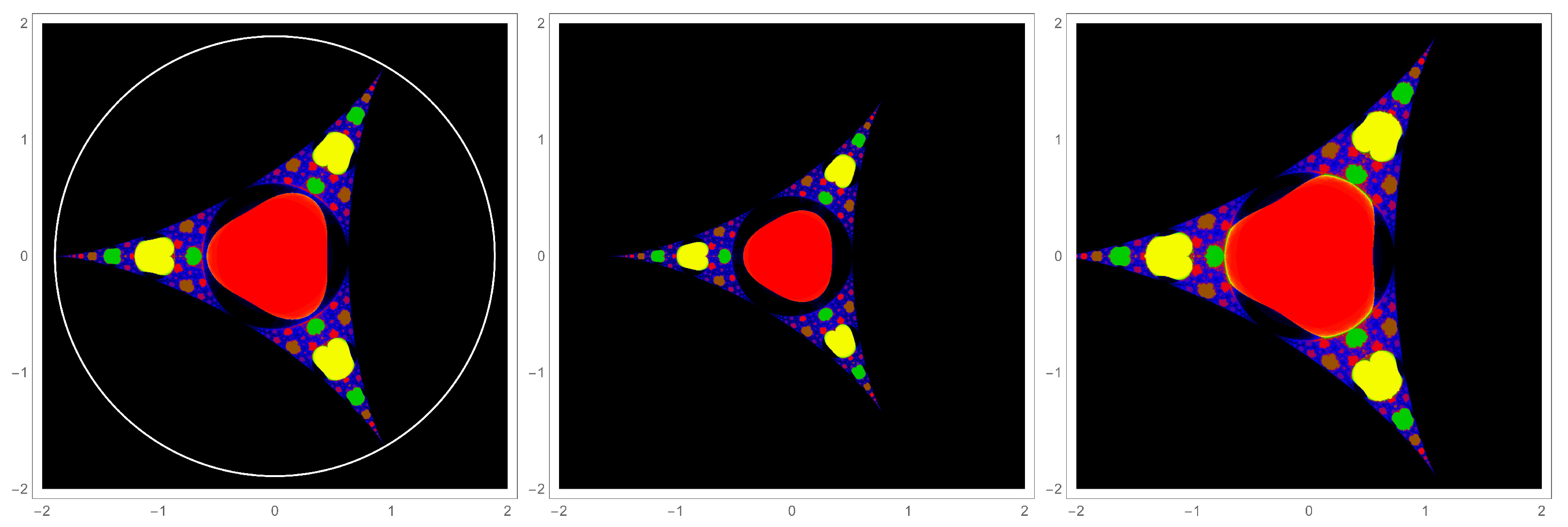
The left most panel of Figure 1 shows the j-averaged Mandelbrot set for the simple inversion case, ${\mu }^{\left(I\right)}=\frac{1}{z}$ ($I=(0,1,1,0)$) for $j=100$. The three-fold rotational symmetry and the three dihedral mirror planes are immediately evident and will be proven below. Another prominent feature is the presence of single-color domains, red, yellow, green, etc. These domains are very smooth. It so happens that the j-averaged Mandelbrot set for this case is circumscribed by a circle whose radius is numerically found to be $r=1.889090$ (white circle in Figure 1). The authors were unable to discover an analytic expression for this radius.  

One can introduce a scaling factor $\sigma$, ${\mu }^{\left(A\right)}=\frac{\sigma }{z}$ ($I=(0,\sigma ,1,0)$). The middle panel of Figure 1 shows a contraction ($\sigma =0.75$), while the right panel shows a dilation ($\sigma =1.25$). Though the overall appearances of these j-averaged Mandelbrot sets are similar, they are not simply scaled versions of the simple inverse case. The most notable change is the size of the central red domain relative to the encircling black region. For contractions, there is open black space completely surrounding the red central region.

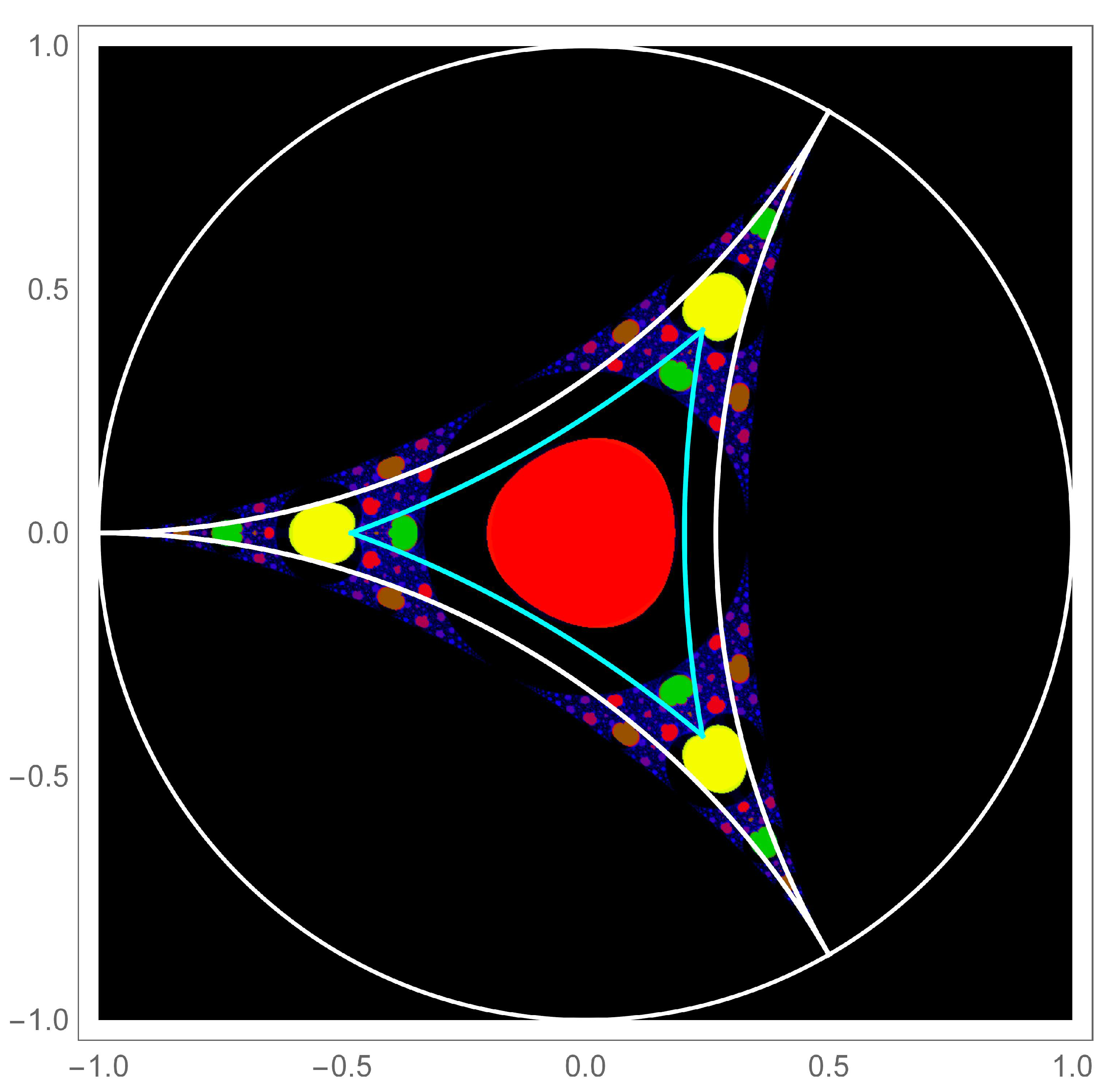
One can numerically find a scaling factor that contracts the resulting j-averaged Mandelbrot set such that it is circumscribed by the unit circle. The scaling factor is $\sigma =0.3851450$ and thus ${\mu }^{\left(U\right)}=\frac{0.3851450}{z}$ ($U\equiv A=(0,0.3851450,1,0)$). The j-averaged Mandelbrot set is plotted in Figure 2. The shape of this set is quite reminiscent of a hyperbolic triangle on the Poincaré disk [4]. The ideal regular triangle formed from the contact points of the j-averaged Mandelbrot set and the unit circle ($-1,e^{\frac{i\pi }{3}},e^{\frac{-i\pi }{3}}$) is superimposed as the white triangle.

The active part of the j-averaged Mandelbrot set is not, in fact, inscribed by the white hyperbolic triangle. Nonetheless, there are some quite interesting connections to the hyperbolic geometry of the Poincaré disk. The geodesic sides of the ideal regular triangle are tangent to the yellow domain. Figure 3 shows a blow-up of this area where the tangency is evident. Each of the yellow domains have a cleft on the proximal side, which shown more clearly in Figure 3. When these clefts are connected by a hyperbolic triangle (cyan triangle in Figure 2), the geodesics of the sides are tangent to the interior green regions. As the top left panel of Figure 3 reveals, there is actually a red corona around the green regions, and the geodesics are tangent to that corona. The central red domain is close to but not tangent to the sides of the cyan triangle, but it is entirely in the interior of the triangle.

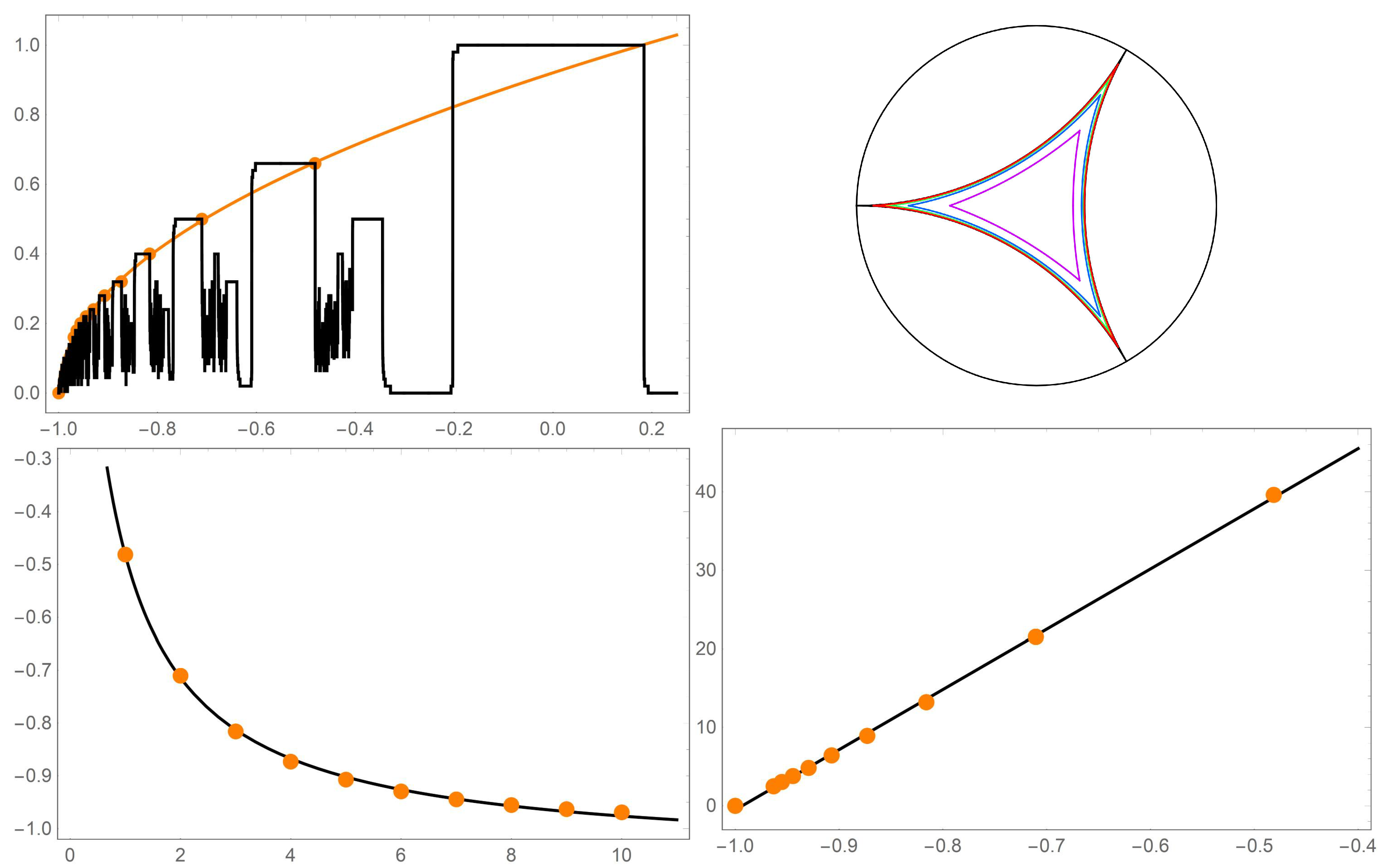
There are outer green domains similar to each of the yellow domains. They, too, have a cleft on the proximal side which form the vertices of another hyperbolic triangle. This is shown as the magenta colored geodesics in the bottom right panel of Figure 3. Although fairly small in the figure, these are seen to be tangent to a small red domain between the distal green domain and the yellow domain. This continues, producing a family of triangles. Five of those triangles are shown in the top right panel of Figure 4.

To better understand these hyperbolic triangles, the positions of the clefts of each subsequent domain, i.e., yellow, green, brown, etc., were determined numerically. Figure 4 captures the results of this analysis. The top right graph shows a one-dimensional slice along the real axis of the j-averaged Mandelbrot set shown in Figure 2 and Figure 3. The cleft positions are marked with orange dots. These data were fit to a single parameter function, $f=C\sqrt{x+1}$, the orange curve that shows remarkable agreement. The bottom left black curve shows a best fit of $f=\frac{C}{x+x_0}+C_0$ to the position versus domain number (counting outward from the center starting with the yellow domain). Finally, and not unexpectedly, there is a linear relationship between the position of the clefts and the interior angles of the hyperbolic triangles.

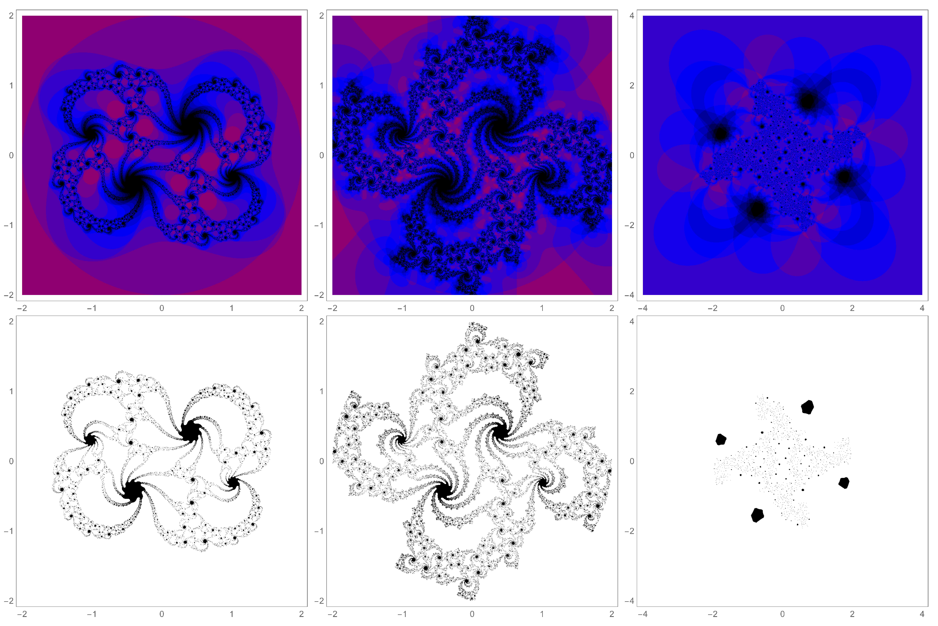
The effect of the three-fold and dihedral mirror symmetries of the j-averaged Mandelbrot set on the j-averaged filled-in Julia set is illustrated in Figure 5. The choice of $\lambda =-0.45+0.05i$ is used as the concrete example and is shown in the top left panel. This particular j-averaged filled-in Julia set has a blue porous appearance on a red background. Analytically, this indicates that, for this value of $\lambda$, many points are in the odd/even alternating set as j changes (red), and the rest of the others are a bit more often in the filled-in Julia set than not (blue). There do not appear to be any points that are always in the filled-in Julia set (those points would appear as black).

Moving across the top row of Figure 5 shows the corresponding $\lambda$ from each of the two other arms in the j-averaged Mandelbrot set: that is, $e^{\frac{2\pi }{3}}\lambda$ (top, middle) and $e^{\frac{-2\pi }{3}}\lambda$ (top, right). The j-averaged filled-in Julia sets are identical aside from a rotation.

The middle row of Figure 5 shows the j-averaged filled-in Julia sets corresponding to reflecting $\lambda$ across the dihedral mirror plane of the arm of the j-averaged Mandelbrot set it is drawn from: for example, $\lambda =-0.45-0.05i$ (the middle left panel).

Finally, it is interesting to compare with the simple inversion case ($A\equiv I=(0,1,1,0)$). This is done in the bottom row of Figure 5. Here, for example, the value of $\lambda$ in the bottom left panel is $1.889090\times (-0.45+0.05i)$ (note, $1.889090$ is the radius of the white circle in Figure 1). Indeed, the resulting j-averaged filled-in Julia sets shown across the bottom row have a similar appearance and orientation to those across the top row. One distinction is the appearance of the small green domains in each of the corners of the filled-in Julia set. These points are not in the filled-in Julia sets as j changes as often as their counter parts in the scaled inversion case. A second and perhaps more curious feature is that although the j-averaged filled-in Julia sets are bigger, they are only approximately 1.35 times bigger. This is smaller than the 1.889090 scale factor of $\lambda$ but is roughly its square root: $\sqrt{1.889090}=1.374417$.

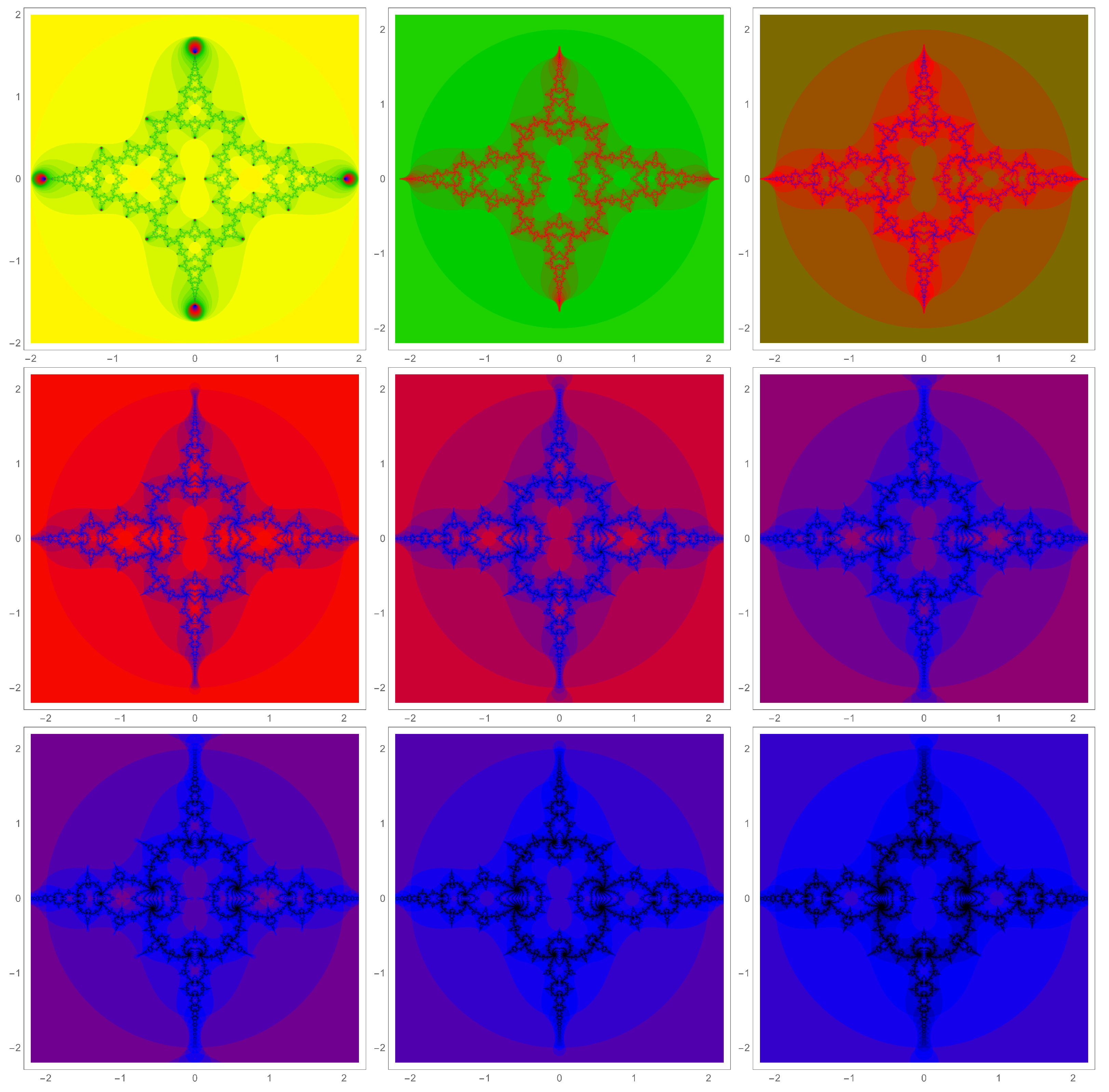
Returning to position of the nexus of the cleft for each of the yellow, green, brown, etc., domains in Figure 2, which are plotted as orange points in Figure 4, there is some interesting correspondence between the j-averaged filled-in Julia sets. The j-averaged filled-in Julia sets for the first nine of these points are collected in Figure 6. A first point of note is that the background color is the same as the color of the domain in the j-averaged Mandelbrot set as most clearly seen in Figure 3. Thus, most of the points in the j-averaged filled-in Julia set behave as they do in the local region in the j-averaged Mandelbrot set.

A second point of note is the symmetry of these structures. They have twofold rotational symmetry and dihedral mirror symmetry. However, there is a quasi-fourfold rotational symmetry present. Each figure has the appearance of a hyperbolic quadrilateral (this is just a descriptor to help guide the eye). Connecting the sides of this quadrilateral are strands running across each arm. Interestingly, as one goes from domain 1 (yellow) to 2 (green), each path bifurcates into two paths. This continues such that the number of paths is equal to the domain number. A final point of note is the scale. Each j-averaged filled-in Julia set is roughly the same size, even though the size of the domains in the j-averaged Mandelbrot set are monotonically decreasing.

Figure 7 shows a few j-averaged filled-in Julia sets in which the filled-in Julia set itself plays a prominent role in the appearance. The top row shows the j-averaged filled-in Julia sets, whereas the bottom row shows the filled-in Julia sets. The filled-in Julia sets are intricate and elaborate.

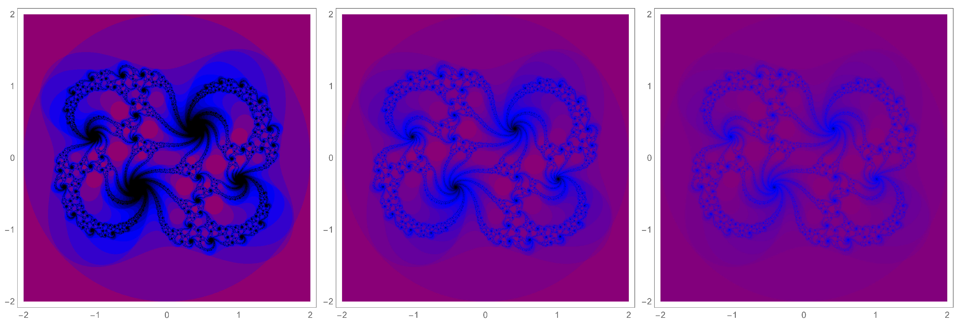
It is important to note, however, that, in a sense, Figure 7 is misleading. As j increases, the filled-in Julia set is whittled away as points along its edges fall out of the set. Eventually this outstrips the resolution of the plots, and the filled-in Julia sets disappear. This is illustrated in Figure 8. The leftmost panel is a repeat of the top left panel of Figure 7. In this case $j=100$. The middle panel shows $j=250$, and the right panel shows $j=500$. At a resolution of a one million point square lattice sampling, only the points in the eyes of the swirls remain black.

In addition to the qualitative description just presented, one can place the rotational and dihedral mirror plan symmetry on a firm foundation. This is done via the following theorem.

Theorem 1.

The j-averaged Mandelbrot set for $\eta \left(z\right)=z^2+\lambda$ has threefold rotational symmetry and dihedral mirror symmetry.

Proof. 

The proof is obtained by a direct calculation and recognition of a pattern, directly from the iteration process

$${\mathcal{H}}_0=\left\{0,\frac{1}{\lambda },\frac{1}{\frac{1}{{\lambda }^2}+\lambda },\frac{1}{\frac{1}{{\left(\frac{1}{{\lambda }^2}+\lambda \right)}^2}+\lambda },\frac{1}{\frac{1}{{\left(\frac{1}{{\left(\frac{1}{{\lambda }^2}+\lambda \right)}^2}+\lambda \right)}^2}+\lambda },\cdots \right\}.$$

(4)

Note that the symmetry of the j-averaged Mandelbrot set at a given value of j arises from the symmetry of the modulus of elements of ${\mathcal{H}}_0$ up to the jth term. The modulus of the first two elements of ${\mathcal{H}}_0$ is isotropic and thus does not contribute to the symmetry. The third term can be written as

$$\begin{array}{c}\hfill \left|\frac{1}{\frac{1}{{\lambda }^2}+\lambda }\right|=\left|\frac{{\lambda }^2}{1+{\lambda }^3}\right|=\left|{\lambda }^2\right|·\left|\frac{1}{1+{\lambda }^3}\right|.\end{array}$$

(5)

The first factor in the last term is also isotropic, but the second factor has threefold rotational symmetry (and dihedral mirror symmetry). In fact, it has poles at $-1$, $e^{\frac{\pi i}{3}}$, and $e^{\frac{-\pi i}{3}}$.

Now, set

$${\chi }_1\equiv \frac{1}{\frac{1}{{\lambda }^2}+\lambda }$$

(6)

for convenience, and consider the fourth member of ${\mathcal{H}}_0$:

$$\begin{array}{c}\hfill \left|\frac{1}{\frac{1}{{\left(\frac{1}{{\lambda }^2}+\lambda \right)}^2}+\lambda }\right|=\left|\frac{1}{{\chi }_1^2+\lambda }\right|\end{array}$$

(7)

which has threefold symmetry and dihedral mirror symmetry.

This process is can be continued as

$${\chi }_2\equiv \frac{1}{{\chi }_1^2+\lambda },$$

(8)

which, for the modulus of the fifth member of ${\mathcal{H}}_0$, gives

$$\left|\frac{1}{{\chi }_2^2+\lambda }\right|.$$

(9)

Repeating this procedure gives a sequence that is fully threefold rotationally symmetric with three dihedral mirrors, thus completing the proof.    □

One can go even further and consider the coefficients on the ${\lambda }^n$ terms in the nested series as $j\to \infty$. This leads to the following conjecture that is awaiting a formal proof.

Conjecture 2.

Let ${\mathcal{H}}_0$ be the sequence of iterated functions in Equation (4) in which the jth member of this sequence, ${}^j{h}^{\left(I\right)}\left(z\right)$, is given by Equation (2) (with $A=I$). Then, for even j ($j=2k$):

$$\underset{k\to \infty }{lim}{}^{2k}{h}^{\left(I\right)}\left(z\right)=\sum _{n=1}^{\infty }{C}_{n-1}{\lambda }^{3n-1}$$

(10)

and even j ($j=2k+1$):

$$\underset{k\to \infty }{lim}{}^{2k+1}{h}^{\left(I\right)}\left(z\right)=\frac{1}{\lambda }-\sum _{n=1}^{\infty }{C}_{n-1}{\lambda }^{3n-1}$$

(11)

where $C_n$ is the nth Catalan number. The disk of convergence is $0<\left|\lambda \right|<1$.

A justification (but not a proof) of this conjecture is as follows. Begin by considering the third member of ${\mathcal{H}}_0$ and expressing it as a series:

$$\begin{array}{c}\hfill \frac{1}{\frac{1}{{\lambda }^2}+\lambda }=\frac{{\lambda }^2}{1+{\lambda }^3}={\lambda }^2\left(1-{\lambda }^3+{\lambda }^6+\cdots \right),\end{array}$$

(12)

where the geometric series was recognized and employed in going to the last expression. For convenience, let $s=\left(1-{\lambda }^3+{\lambda }^6+\cdots \right)$. Notice that only the powers of multiples of three are active in s. Thus, this member of ${\mathcal{H}}_0$ has threefold symmetry and dihedral symmetry (consistent with Theorem 1).

Likewise, one can develop a series expression for the fourth term as

$$\begin{array}{cc}\hfill \frac{1}{\frac{1}{{\left(\frac{1}{{\lambda }^2}+\lambda \right)}^2}+\lambda }& =\frac{1}{\lambda +\frac{{\lambda }^4}{1+{\lambda }^3}}\hfill \\ \hfill & =\frac{1}{\lambda +\lambda \left({\lambda }^{3}s\right)}=\frac{1}{\lambda }\left(\frac{1}{1+{\lambda }^{3}s}\right)\hfill \\ \hfill & =\frac{1}{\lambda }\left(1-{\lambda }^{3}s+{\lambda }^6{s}^2\cdots \right).\hfill \end{array}$$

(13)

This is now a series of series, but, nonetheless, the overall series contains only powers of $\lambda$ that are multiples of three. This process is continued for j iterations. If j is odd, there will be a leading term of ${\lambda }^{-1}$, and if j is even, the leading term will be ${\lambda }^2$. In each case, the powers of the remaining terms increase by 3. The heavily nested series quickly becomes unwieldy to handle analytically. This can be aided by the use of Mathematica to produce the coefficients in succession, which are the Catalan numbers for the first $\frac{j}{2}$ terms, after which they deviate from the Catalan numbers. For example, the series expansion for the $j=10$ case is ($C_{\frac{j}{2}-1}$ underlined)

$${\lambda }^2+{\lambda }^5+2{\lambda }^8+5{\lambda }^{11}+\underline{14}{\lambda }^{14}-470{\lambda }^{17}+388{\lambda }^{20}+\cdots$$

(14)

and for the $j=20$ case, it is

$$\begin{array}{cc}\hfill {\lambda }^2& +{\lambda }^5+2{\lambda }^8+5{\lambda }^{11}+14{\lambda }^{14}+42{\lambda }^{17}+132{\lambda }^{20}+429{\lambda }^{23}+1430{\lambda }^{26}\hfill \\ \hfill & +\underline{4862}{\lambda }^{29}-507492{\lambda }^{32}+320930{\lambda }^{35}+\cdots \hfill \end{array}$$

(15)

Similarly for odd values of j, one finds, for example, for $j=21$

$$\begin{array}{cc}\hfill \frac{1}{\lambda }& -{\lambda }^2-{\lambda }^5-2{\lambda }^8-5{\lambda }^{11}-14{\lambda }^{14}-42{\lambda }^{17}-132{\lambda }^{20}-429{\lambda }^{23}\hfill \\ \hfill & -1430{\lambda }^{26}-\underline{4862}{\lambda }^{29}+1031780{\lambda }^{32}-1631650{\lambda }^{35}+\cdots \hfill \end{array}$$

(16)

5. Conclusions

The classic fractal $\eta =z^2+\lambda$ was generalized to include a fixed Möbius transformation at each iteration step. The nature of the filled-in Julia sets and the Mandelbrot sets for these fractals was the central focus of this work. Special cases of affine transformations and inversions were studied in detail.

While the affine transformations did not give rise to much surprise, the inversion subgroup led to interesting rotational and dihedral mirror symmetry in the Mandelbrot set. There was also a connection to hyperbolic triangles in the Poincaré disk. It proved convenient to define j-averaged Mandelbrot and j-averaged filled-in Julia sets to better illustrate the effects of inversion.

Three possible extensions of the current work could be to explore other subgroups of Möbius transformations, to study a different base function than $\eta =z^2+\lambda$, or to let the Möbius transformation change with each iteration.

References

- Peitgen, H.-O.; Jürgens, H.; Saupe, D. Chaos and Fractals, 2nd ed.; Springer: New York, NY, USA, 2004. [Google Scholar]
- Falconer, K. Fractal Geometry: Mathematical Foundations and Applications, 2nd ed.; Wiley: Chichester, UK, 2004. [Google Scholar]
- Barnsley, M. Fractals Everywhere, 2nd ed.; Academic Press: Boston, MA, USA, 1993. [Google Scholar]
- Lyndon, R.C. Groups and Geometry; Cambridge University Press: Cambridge, UK, 1985. [Google Scholar]
- Beals, R.; Wong, R.S. Explorations in Complex Functions; Springer: New York, NY, USA, 2020. [Google Scholar]
- Katok, S. Fuchsian Groups; University Chicago Press: Chicago, IL, USA, 1992. [Google Scholar]
- Feijs, L.; Toeters, M. Exploring a taxicab-based Mandelbrot-like set. In Bridges 2019 Conference Proceedings; Johannes Kepler University: Linz, Austria, 2019. [Google Scholar]
- Teoters, M.; Feijs, L.M.G.; Van Loenhout, D.; Tieleman, C.; Virtala, N.; Jaakson, G.K. Algorithmic fashion aesthetics: Mandelbrot. In Proceedings of the ISWC ’19: 23rd International Symposium on Wearable Computers, London, UK, 11–13 September 2019. [Google Scholar]
- Yadav, A.; Rani, M.; Verma, V.K.; Mundra, A. A review on controlling of Julia and Mandelbrot sets. Int. J. Adv. Sci. Technol. 2019, 28, 213–223. [Google Scholar]
- Xiang, Z.; Zhou, K.-Q.; Guo, Y. Gaussian mixture noised random fractals with adversarial learning for automated creation of visual objects. Fractals 2020, 28, 2050068. [Google Scholar] [CrossRef]
- Kwun, K.C.; Tanveer, M.; Nazeer, W.; Gdawiec, K.; Kang, S.M. Mandelbrot and Julia Sets via Jungck-CR Iteration with s-Convexity. IEEE Access 2019, 7, 12167–12176. [Google Scholar] [CrossRef]
- Kwun, K.C.; Tanveer, M.; Nazeer, W.; Abbas, M.; Kang, S.M. Fractal generation in modified Jungck-S orbit. IEEE Access 2019, 7, 35060–35071. [Google Scholar] [CrossRef]
- Li, D.; Tanveer, M.; Nazer, W.; Guo, X. Boundaries of filled Julia Sets in generalized Jungck Mann orbit. IEEE Access 2019, 7, 76859–76867. [Google Scholar] [CrossRef]
- Abbas, M.; Iqbal, H.; De la Sen, M. Generation of Julia and Mandelbrot Sets via Fixed Points. Symmetry 2020, 12, 1797. [Google Scholar] [CrossRef]
- Tan, L. Similarity between the Mandelbrot Set and Julia Sets. Commun. Math. Phys. 1990, 134, 587–617. [Google Scholar]
- Kawahira, T. Zalcman functions and similarity between the Mandelbrot set, Julia sets, and the tricorn. Anal. Math. Phys. 2020, 10, 16. [Google Scholar] [CrossRef] [Green Version]
- Blankers, V.; Rendfrey, T.; Shukert, A.; Shipman, P.D. Julia and Mandelbrot Setsfor Dynamics over the Hyperbolic Numbers. Fractal Fract. 2019, 3, 6. [Google Scholar] [CrossRef] [Green Version]
- Chaves, A.P.; Trojovský, P. A quadratic Diophantine equation involving generalized Fibonacci numbers. Mathematics 2020, 8, 1010. [Google Scholar] [CrossRef]
- Drakopoulos, V. Comparing rendering methods for Julia sets. J. WSCG 2002, 10, 155–161. [Google Scholar]
- Drakopoulos, V. Sequential visualisation methods for the Mandelbrot set. JCMSE 2010, 10, 37–45. [Google Scholar] [CrossRef]
- Mork, L.K.; Vogt, T.; Sullivan, K.; Rutherford, D.; Ulness, D.J. Exploration of filled-in Julia sets arising from centered polygonal lacunary functions. Fractal Fract. 2019, 3, 42. [Google Scholar] [CrossRef] [Green Version]
- Mork, L.K.; Sullivan, K.; Ulness, D.J. Lacunary Möbius fractals on the unit disk. Symmetry 2021, 13, 91. [Google Scholar] [CrossRef]
- Mathematica 12; Wolfram Research: Champaign, IL, USA, 2020.
Figure 1.
The j-averaged Mandelbrot set for simple inversion (left panel: ) and scaled inversion (middle panel: and right panel: ). A circle of radius circumscribes the simple inversion Mandelbrot set. Scaling with a number less than 1 leads to a smoothing of the Mandelbrot set relative to the unscaled set. Conversely, scaling by a factor greater than 1 leads to greater roughness of the set.
Figure 2.
Hyperbolic geometric features of . When the ideal regular triangle (white) is inscribed on the unit disk, the hyperbolic geodesics are tangent to the three larger orbiting domains. Figure 3 shows a blow-up of this region. The three pronounced yellow orbiting domains have an inward pointing mouth (see Figure 3) which form the vertices of the hyperbolic triangle shown in cyan (angles: ). The cyan geodesics are nearly but not tangent with the central domain (red) but they are tangent to the coronas of the inner green regions (see Figure 3).
Figure 3.
Several blow-ups on one of three arms of the j-averaged Mandelbrot set in Figure 2. The top two panels reveal the tangency to the geodesics of the ideal regular triangle shown in white in Figure 2 and the cyan-colored hyperbolic triangle formed from the clefts of the yellow domains. The bottom left panel shows a blow-up of the cleft region of the yellow domain. The j-averaged Mandelbrot set is quite active in the region emerging from the nexus of the cleft. The bottom right panel shows two sequential blow-ups of the tail of the arm of the j-averaged Mandelbrot set.
Figure 4.
Numerical fits for several features associated with the j-averaged Mandelbrot set for . The top left graph shows a linear slice of the Mandelbrot set for . The ordinate is a normalized scale representing the amount of times a point is not in the Mandelbrot set; 1 is the red domain in Figure 2, 0.667 is the yellow, 0.5 is the green, etc. The orange points are the values of at the proximal cleft of each domain. The orange line is the fit of to these data (best fit parameter ). The bottom left shows the position of the cleft (ordinate) versus the domain number (abscissa). The data are fit to (best fit parameters , , and ). The top right shows the first five hyperbolic triangles defined by the positions of the clefts. The bottom right graph shows the angle of the hyperbolic triangles (ordinate) versus position of the cleft (abscissa). The data are fit to (best fit parameters , ).
Figure 5.
Nature of the three-fold symmetry of the j-averaged Mandelbrot set on the j-averaged filled-in Julia sets. The top left panel shows the j-averaged filled-in Julia corresponding to . The top middle and right panels show and , respectively. The second row shows the j-averaged filled-in Julia sets corresponding to reflecting across the respective dihedral mirrors. The bottom row shows the j-averaged filled-in Julia set coming from the simple inversion case (). Each respective value of is times that from the top row. The j-averaged filled-in Julia sets look similar but not identical, and they are about 1.35 times bigger.
Figure 6.
j-averaged filled-in Julia sets from points in the j-averaged Mandelbrot sets at positions of the orange data points in Figure 4. Domains 1 through 9 are shown. The appearance has significant similarities. One important difference is that the number of strands crossing from one side of an arm to the other is equal to the domain number.
Figure 7.
A few intricate and impressive looking j-averaged filled-in Julia sets coming from the mouth regions of one of the three larger orbiting domains. For all plots , sampled as a 1M pt square lattice. Top left , top middle, , top right . The bottom row simply shows the filled-in Julia set.
Figure 8.
Effect of j on the appearance of the j-averaged filled-in Julia set associated with for (left-to-right) , , and . The set of points that are always in the filled-in Julia sets tighten up with increasing j.
Publisher’s Note: MDPI stays neutral with regard to jurisdictional claims in published maps and institutional affiliations. |
© 2021 by the authors. Licensee MDPI, Basel, Switzerland. This article is an open access article distributed under the terms and conditions of the Creative Commons Attribution (CC BY) license (https://creativecommons.org/licenses/by/4.0/).
Share and Cite
MDPI and ACS Style
Mork, L.K.; Ulness, D.J. Visualization of Mandelbrot and Julia Sets of Möbius Transformations. Fractal Fract. 2021, 5, 73. https://0-doi-org.brum.beds.ac.uk/10.3390/fractalfract5030073
AMA Style
Mork LK, Ulness DJ. Visualization of Mandelbrot and Julia Sets of Möbius Transformations. Fractal and Fractional. 2021; 5(3):73. https://0-doi-org.brum.beds.ac.uk/10.3390/fractalfract5030073
Chicago/Turabian StyleMork, Leah K., and Darin J. Ulness. 2021. "Visualization of Mandelbrot and Julia Sets of Möbius Transformations" Fractal and Fractional 5, no. 3: 73. https://0-doi-org.brum.beds.ac.uk/10.3390/fractalfract5030073