A Nonlocal Fractional Peridynamic Diffusion Model

Abstract

This paper proposes a nonlocal fractional peridynamic (FPD) model to characterize the nonlocality of physical processes or systems, based on analysis with the fractional derivative model (FDM) and the peridynamic (PD) model. The main idea is to use the fractional Euler–Lagrange formula to establish a peridynamic anomalous diffusion model, in which the classical exponential kernel function is replaced by using a power-law kernel function. Fractional Taylor series expansion was used to construct a fractional peridynamic differential operator method to complete the above model. To explore the properties of the FPD model, the FDM, the PD model and the FPD model are dissected via numerical analysis on a diffusion process in complex media. The FPD model provides a generalized model connecting a local model and a nonlocal model for physical systems. The fractional peridynamic differential operator (FPDDO) method provides a simple and efficient numerical method for solving fractional derivative equations.

1. Introduction

In recent decades, nonlocal models have attracted increasing attention for dealing with complex physical problems [1,2,3,4]. The applications of nonlocal models have been reported in various research areas, such as groundwater flow in heterogeneous porous media [5], heat conduction in composite materials [6], and the deformations of heterogeneous materials [7]. Numerical discretization of a traditional local model usually yields many degrees of freedom, which leads to excessive calculations and increases the computational complexity, despite providing low accuracy [8,9]. Therefore, nonlocal models have been proposed to facilitate numerical analysis [10,11,12].

As a nonlocal model, the fractional derivative model (FDM) has been widely used to describe the temporal history-memory and spatial nonlocality of physical behaviors [13,14,15,16]. Compared with the integer-order derivative model, the FDM has achieved great success in characterizing various anomalous phenomena in the physics and engineering fields [17,18,19]. Moreover, different power-law tail phenomena can be accurately documented by employing fractional derivative models, thanks to the nonlocal property of the fractional operator [20,21]. However, its application is hindered by the heavy computational burden of numerical simulations [22,23,24].

The peridynamic (PD) model is a newly developed nonlocal approach, the original prototype of which was conceived by Silling in 2000 [25,26]. In recent years, the PD model has been successfully applied to resolve various static and dynamic problems of different materials [27,28,29,30] and multi-scale problems [31,32,33]. The peridynamic differential operator (PDDO) is obtained by multiplying the kernel function with a Taylor series expansion of neighborhood field variables, and then integrating them in the interaction domain with orthogonality [34,35,36]. As a typical meshless method, the PDDO can greatly reduce the computational burden [37,38]. However, compared with the globally-dependent fractional derivative model, many nonlocal processes cannot be fully described by using the PD model, due to its limitation in the selection of memory area [39,40].

To combine the advantages of the FDM and the PD model, this paper attempts to introduce a fractional peridynamic (FPD) model to characterize different degrees of nonlocality. The FPD diffusion equation was constructed by employing the fractional Euler–Lagrange formula. The corresponding fractional peridynamic differential operator (FPDDO) was established with the help of a generalized Taylor series expansion. Since the FPDDO method can directly solve the fractional equation, the FPD model avoids the complex expression and heavy computational burden of the FDM. In the FPD model, the classical exponential kernel function of the PD model is replaced by a power-law kernel function. Therefore, the FPD model can describe different degrees of nonlocality via changing the index of the power-law kernel function and the size of the near-field range. Furthermore, here the PD model and FPD model are used to solve the diffusion process by considering a numerical example, to explore its advantages and characteristics.

The rest of this paper is organized as follows. In Section 2, the FPD model and the FPDDO are introduced. In Section 3, a numerical example is given to verify the accuracy of the FPD model with a power-law function kernel and discuss its nonlocality. Finally, some conclusions and remarks are provided in Section 4.

2. Materials and Methods

2.1. The FPD Anomalous Diffusion Model

Fick’s law to describe diffusion in porous media can be expressed as

$$J=-D\frac{dC}{dx},$$

(1)

in which $J$ is the diffusion flux, $D$ is the diffusion coefficient, $C$ is the concentration, and $dC/dx$ represents the concentration gradient [41].

The governing equation of diffusion is derived from the Euler–Lagrange equation. To introduce the FPD model, we first give the expression of fractional Lagrange function [42]:

$$L=L\left(t,C\left(x,t\right),C^{\left(\alpha \right)}\left(x,t\right)\right),\hspace{1em}\hspace{1em}\left(0<\alpha \le 1\right),$$

(2)

where $C^{\left(\alpha \right)}\left(x,t\right)=\frac{d^{\alpha }C\left(x,t\right)}{d{x}^{\alpha }}$; when $\alpha =1$, Equation (2) reduces to the classical Lagrange function. Based on the fractional Lagrange function, the fractional Euler–Lagrange equation can be given as

$$\frac{d}{dt}\left(\frac{\partial L}{\partial \left(C^{\left(\alpha \right)}\left(x,t\right)\right)}\right)-\frac{\partial L}{\partial C\left(x,t\right)}=0,\hspace{1em}\hspace{1em}\left(0<\alpha \le 1\right).$$

(3)

For the node $x_{\left(k\right)}$, assume the Lagrange function to be

$$L=T-V,$$

(4)

where $T$ and $V$ represent the kinetic and potential energies, respectively. In the hydrodynamic approach, molecular diffusion needs to satisfy the momentum equation for constant flow:

$$F={\displaystyle {\mathsf{\oint }}_{cs}C(\rho CdA)},$$

(5)

where $\rho$ is the fluid density and $\rho =1.0{\mathrm{kg}/\mathrm{m}}^3$. By summing the kinetic energy and potential energy of all particles [43], we can get

$$T={\displaystyle \sum _{k=1}^{\infty }\frac{1}{2}}C\left(C{V}_{\left(k\right)}\right),$$

(6)

and

$$V={\displaystyle \sum _{k=1}^{\infty }{W}_{\left(k\right)}{V}_{\left(k\right)}}-{\displaystyle \sum _{i=1}^{\infty }\left[b_{\left(k\right)}·C_{\left(k\right)}\right]V_{\left(k\right)}},$$

(7)

where $b_{\left(k\right)}$ is the particle source intensity representing the amount of particles produced by the particle source term per unit time and volume, and $W_{\left(k\right)}$ is the molecular potential energy of all nodes interacting with node $x_{\left(k\right)}$. Here we define: (1) $w_{\left(k\right)\left(j\right)}=w_{\left(k\right)\left(j\right)}\left(C_{\left(1^k\right)}-C_{\left(k\right)},C_{\left(2^k\right)}-C_{\left(k\right)},\cdots \right)$ and $w_{\left(j\right)\left(k\right)}=w_{\left(j\right)\left(k\right)}\left(C_{\left(1^j\right)}-C_{\left(j\right)},C_{\left(2^j\right)}-C_{\left(j\right)},\cdots \right)$; (2) $w_{\left(k\right)\left(j\right)}$ depends on the concentration difference between point $x_{\left(k\right)}$ and all interacting points; (3) $C_{\left(k\right)}$ is the concentration of point $x_{\left(k\right)}$; (4) $C_{\left(1^k\right)}$ denotes the concentration of the first point interacting with point $x_{\left(k\right)}$. Then $W_{\left(k\right)}$ is defined as

$$W_{\left(k\right)}=\frac{1}{2}{\displaystyle \sum _{j=1}^{\infty }\frac{1}{2}}\left[\begin{array}{l}{w}_{\left(k\right)\left(j\right)}\left(C_{\left(1^k\right)}-C_{\left(k\right)},C_{\left(2^k\right)}-C_{\left(k\right)},\cdots \right)+\\ w_{\left(j\right)\left(k\right)}\left(C_{\left(1^j\right)}-C_{\left(j\right)},C_{\left(2^j\right)}-C_{\left(j\right)},\cdots \right)\end{array}\right]V_{\left(j\right)}.$$

(8)

Based on Equation (8), Equation (7) can be rewritten as

$$V={\displaystyle \sum _{k=1}^{\infty }\left\{\frac{1}{2}{\displaystyle \sum _{j=1}^{\infty }\frac{1}{2}\left[\begin{array}{l}{w}_{\left(k\right)\left(j\right)}\left(C_{\left(1^k\right)}-C_{\left(k\right)},C_{\left(2^k\right)}-C_{\left(k\right)},\cdots \right)+\\ w_{\left(j\right)\left(k\right)}\left(C_{\left(1^j\right)}-C_{\left(j\right)},C_{\left(2^j\right)}-C_{\left(j\right)},\cdots \right)\end{array}\right]V_{\left(j\right)}-\left[b_{\left(k\right)}·C_{\left(k\right)}\right]}\right\}{V}_{\left(k\right)}}.$$

(9)

By substituting Equations (6) and (9) into Equation (4), the Lagrange function can be expressed as

$$L={\displaystyle \sum _{k=1}^{\infty }\left\{\frac{1}{2}{C}_{\left(k\right)}·C_{\left(k\right)}-\frac{1}{2}{\displaystyle \sum _{j=1}^{\infty }\frac{1}{2}\left[\begin{array}{l}{w}_{\left(k\right)\left(j\right)}\left(C_{\left(1^k\right)}-C_{\left(k\right)},C_{\left(2^k\right)}-C_{\left(k\right)},\cdots \right)\\ +w_{\left(j\right)\left(k\right)}\left(C_{\left(1^j\right)}-C_{\left(j\right)},C_{\left(2^j\right)}-C_{\left(j\right)},\cdots \right)\end{array}\right]V_{\left(j\right)}+b_{\left(k\right)}{C}_{\left(k\right)}}\right\}}{V}_{\left(k\right)}.$$

(10)

Then, Equation (3) leads to the fractional Euler–Lagrange equation as such:

$${\dot{u}}_{\left(k\right)}={\displaystyle \sum _{j=1}^{\infty }\frac{1}{2}\left\{{\displaystyle \sum _{i=1}^{\infty }\frac{{\partial }^{\alpha }{w}_{\left(k\right)\left(i\right)}}{\partial {\left(C_{\left(j\right)}-C_{\left(k\right)}\right)}^{\alpha }}}{V}_{\left(i\right)}\right\}}-{\displaystyle \sum _{j=1}^{\infty }\frac{1}{2}\left\{{\displaystyle \sum _{i=1}^{\infty }\frac{{\partial }^{\alpha }{w}_{\left(i\right)\left(k\right)}}{\partial {\left(C_{\left(k\right)}-C_{\left(j\right)}\right)}^{\alpha }}}{V}_{\left(i\right)}\right\}}+b_{\left(k\right)},\hspace{1em}\hspace{1em}\left(0<\alpha \le 1\right).$$

(11)

Here we define the fluid density $C^{\left(\alpha \right)}(x,t)\langle x^{\prime }-x\rangle$ and $C^{\left(\alpha \right)}(x^{\prime },t)\langle x-x^{\prime }\rangle$ as

$$\begin{array}{l}{C}^{\left(\alpha \right)}(x,t)\langle x^{\prime }-x\rangle =\frac{1}{2}\frac{1}{V_{\left(j\right)}}\left\{{\displaystyle \sum _{i=1}^{\infty }\frac{{\partial }^{\alpha }{w}_{\left(k\right)\left(i\right)}}{\partial {\left(C_{\left(j\right)}-C_{\left(k\right)}\right)}^{\alpha }}}{V}_{\left(i\right)}\right\},\\ C^{\left(\alpha \right)}(x^{\prime },t)\langle x-x^{\prime }\rangle =\frac{1}{2}\frac{1}{V_{\left(j\right)}}\left\{{\displaystyle \sum _{i=1}^{\infty }\frac{{\partial }^{\alpha }{w}_{\left(i\right)\left(k\right)}}{\partial {\left(C_{\left(k\right)}-C_{\left(j\right)}\right)}^{\alpha }}}{V}_{\left(i\right)}\right\},\end{array}$$

(12)

where $\langle x-x^{\prime }\rangle$ contains interacting pairs of particles, and clearly fluid density is a function of each pair of point sets. With the state notation of Equation (12), Equation (11) can be rewritten as

$$\dot{u}\left(x,t\right)={\displaystyle \sum _{j=1}^{\infty }\left(C^{\left(\alpha \right)}\left(x,t\right)\langle x^{\prime }-x\rangle -C^{\left(\alpha \right)}\left(x^{\prime },t\right)\langle x-x^{\prime }\rangle \right)}{V}_{\left(j\right)}+b\left(x,t\right),\hspace{1em}\hspace{1em}\left(0<\alpha \le 1\right).$$

(13)

When we consider the volume of each particle is infinitesimal, $V_{\left(j\right)}\to 0$, then infinite sums can be approximated by using integral ${\displaystyle \sum _{j=1}^{\infty }()}{V}_{\left(j\right)}\to {\displaystyle {\int }_H()d{V}_{x^{\prime }}}\to {\displaystyle {\int }_H()dH}$. Hereby, the FPD anomalous diffusion model is obtained as

$$\dot{u}\left(x,t\right)={\displaystyle {\int }_H\left[C^{\left(\alpha \right)}\left(x,t\right)\langle x^{\prime }-x\rangle -C^{\left(\alpha \right)}\left(x^{\prime },t\right)\langle x-x^{\prime }\rangle \right]}\mathrm{d}{V}_{x^{\prime }}+b\left(x,t\right),\hspace{1em}\hspace{1em}\left(0<\alpha \le 1\right),$$

(14)

and $C^{\left(\alpha \right)}\left(x,t\right)\langle x^{\prime }-x\rangle =0$ when $x^{\prime }\notin H$. The integral domain $H$ is defined by the horizon of the material point.

In order to fulfill completeness, the kernel function in FPD should satisfy the zeroth-order consistency conditions as

$${\displaystyle \underset{H_x}{\int }{C}_N^0}wd{V}_{x^{\prime }}=1,$$

(15)

where $C_N^0$ is defined as the polynomial function. We recall the fractional binomial formula

$${\displaystyle \sum _{k=0}^{\infty }\left(\begin{array}{c}\gamma \\ k\end{array}\right)z^k}={\left(1+z\right)}^{\gamma },$$

(16)

which is valid for any $\gamma >0$ and complex $\left|z\right|\le 1$. When $z=-1$, Equation (16) can be written as

$${\displaystyle \sum _{k=0}^{\infty }{\left(-1\right)}^k\left(\begin{array}{c}\gamma \\ k\end{array}\right)}=0.$$

(17)

The kernel function in fractional FPD should satisfy the zeroth-order consistency conditions as

$${\displaystyle \underset{H_x}{\int }{\left(x-x^{\prime }\right)}^{-\gamma }\xi d{V}_{x^{\prime }}}=1.$$

(18)

2.2. The Fractional Peridynamic Differential Operator

To solve real-world anomalous diffusion problem, a fractional peridynamic differential operator is necessary for the given fractional peridynamic model. Here we use fractional Taylor series expansion to establish the fractional peridynamic differential operator. The fractional Taylor series expansion is given as [44]

$$f\left(x+\xi \right)={\displaystyle \sum _{n=0}^{\infty }\frac{{\xi }^{n\alpha }}{\Gamma \left(1+n\alpha \right)}}{f}^{\left(n\alpha \right)}\left(x\right)+R^{\alpha }\left(N,x\right),\hspace{1em}\hspace{1em}\left(0<\alpha \le 1\right),$$

(19)

where $f^{\left(n\alpha \right)}\left(x\right)=\frac{d^{n\alpha }f\left(x\right)}{d{x}^{n\alpha }}$, $R^{\alpha }\left(N,x\right)$ is the remainder. When $\alpha =1$, Equation (19) is reduced to the classical Taylor series expansion. If the contribution of the remainder is very small, it can be neglected. In this case, we multiply each term in this expression by a PD function $g_N^P(\xi )\left(P=0,\alpha ,2\alpha ,\dots ,N\alpha \right),$ and integrate over the family of points; then Equation (19) becomes

$$\begin{array}{l}{\displaystyle {\int }_{H_x}f(x+\xi )g_N^P(\xi )d\xi }=f(x){\displaystyle {\int }_{H_x}{g}_N^0(\xi )d\xi }+\frac{{\partial }^{\alpha }f(x)}{\partial x^{\alpha }}{\displaystyle {\int }_{H_x}\frac{1}{\Gamma \left(1+\alpha \right)}}{\xi }^{\alpha }{g}_N^{\alpha }(\xi )d\xi \\ +\frac{{\partial }^{2\alpha }f(x)}{\partial x^{2\alpha }}{\displaystyle {\int }_{H_x}\frac{1}{\Gamma \left(1+2\alpha \right)}{\xi }^{2\alpha }{g}_N^{2\alpha }(\xi )d\xi }+\dots +\frac{{\partial }^{N\alpha }f(x)}{\partial x^{N\alpha }}{\displaystyle {\int }_{H_x}\frac{1}{\Gamma \left(1+N\alpha \right)}{\xi }^{N\alpha }{g}_N^{N\alpha }(\xi )d\xi }.\end{array}$$

(20)

For the two-dimensional case, the fractional Taylor series expansion of a scalar field $f\left(x^{\prime }\right)=f\left(x+\xi \right)$ can be expressed as

$$f(x+\xi )={\displaystyle \sum _{n_1=0}^N{\displaystyle \sum _{n_2=0}^{N-n_1}\frac{1}{\Gamma \left(1+n_1\alpha \right)\Gamma \left(1+n_2\alpha \right)}{\xi }_1^{n_1\alpha }{\xi }_2^{n_2\alpha }}}\frac{{\partial }^{n_1\alpha +n_2\alpha }f(x)}{\partial x_1^{n_1\alpha }\partial x_2^{n_2\alpha }}+R^{\alpha }(N,x),$$

(21)

where $\xi =x^{\prime }-x$, and $R^{\alpha }\left(N,x\right)$ is the remainder. Assuming the remainder is very small, the nonlocal expression of FPD is obtained by using the properties of orthogonal functions:

$$\left\{\begin{array}{c}\frac{{\partial }^{n_1\alpha }f(x)}{\partial x_1^{n_1\alpha }}\\ \frac{{\partial }^{n_2\alpha }f(x)}{\partial x_2^{n_2\alpha }}\\ \frac{{\partial }^{2n_1\alpha }f(x)}{\partial x_1^{2n_1\alpha }}\\ \frac{{\partial }^{2n_2\alpha }f(x)}{\partial x_2^{2n_2\alpha }}\\ \frac{{\partial }^{n_1\alpha +n_2\alpha }f(x)}{\partial x_1^{n_1\alpha }\partial x_2^{n_2\alpha }}\end{array}\right\}={\displaystyle \underset{H_x}{\int }f(x+\xi )\left\{\begin{array}{c}{g}_2^{10}(\xi )\\ g_2^{01}(\xi )\\ g_2^{20}(\xi )\\ g_2^{02}(\xi )\\ g_2^{11}(\xi )\end{array}\right\}}d{x}_{1}d{x}_2,$$

(22)

where $n_i\alpha$ denotes the derivative order. For a node located at $x$, the horizon $\delta$ defines the extent of its family as $H_x=\left\{x^{\prime }\in \left[a=-\delta ,b=\delta \right]\right\}$. According to the orthogonality of the function, the PD function $g_N^P(\xi )\left(P=0,\alpha ,2\alpha ,\dots ,N\alpha \right)$ possess the orthogonality property of

$$\frac{1}{\Gamma \left(1+n_1\alpha \right)\Gamma \left(1+n_2\alpha \right)}{\displaystyle \underset{H_x}{\int }{\xi }_1^{n_1\alpha }{\xi }_2^{n_2\alpha }}{g}_2^{P_1{P}_2}\left(\xi \right)d{x}_{1}d{x}_2={\delta }_{n_1\alpha }{\delta }_{n_2\alpha }.$$

(23)

The $g_2^{P_1{P}_2}\left(\xi \right)\left(P_1,P_2=0,1,2\right)$ is expressed in matrix form as

$$g_2^{P_1{P}_2}(\xi )={\displaystyle \sum _{q_1=0}^2{\displaystyle \sum _{q_2=0}^{2-q_1}{a}_{q_1{q}_2}^{P_1{P}_2}w(\left|\xi \right|){\xi }_1^{q_1\alpha }{\xi }_2^{q_2\alpha }}},$$

(24)

in which $w\left(\left|\xi \right|\right)$ is the kernel function. By substituting Equation (24) into Equation (23), we can get

$${\displaystyle \sum _{q_1=0}^2{\displaystyle \sum _{q_2=0}^{2-q_1}\begin{array}{c}{A}_{\left(n_1{n}_2\right)\left(q_1{q}_2\right)}\end{array}}}{a}_{q_1{q}_2}^{P_1{P}_2}=b_{n_1{n}_2}^{P_1{P}_2},\hspace{1em}\left(n_1,n_2,P_1,P_2=0,1,2\right),$$

(25)

where

$$A_{\left(n_1{n}_2\right)\left(q_1{q}_2\right)}={\displaystyle \underset{H_x}{\int }w(\left|\xi \right|){\xi }_1^{\left(n_1+q_1\right)\alpha }{\xi }_2^{\left(n_2+q_2\right)\alpha }d{x}_{1}d{x}_2},$$

(26)

$$b_{n_1{n}_2}^{P_1{P}_2}=\Gamma \left(1+n_1\alpha \right)\Gamma \left(1+n_2\alpha \right){\delta }_{n_1{p}_1}{\delta }_{n_2{p}_2}.$$

(27)

Then the unknown coefficients can be obtained by solving the above equation.

3. Results

In our numerical analysis of PD and FPD diffusion models, the spatial integral term is discretized by a single-point Gauss quadrature scheme, and then solved by using the PDDO or FPDDO method. The PDDO method employs the exponential function $w\left(\xi \right)=e^{\left(-{\left(2\xi /\delta \right)}^2\right)}$, whereas the FPDDO method adopts the power-law kernel function $w\left(\xi \right)={\left(x^{\prime }-x\right)}^{-\gamma }$. The discretization of the temporal derivative is obtained via finite difference scheme.

The PD diffusion equation can be written as below.

$$\{\begin{array}{l}\frac{\partial C\left(x,t\right)}{\partial t}={\displaystyle {\int }_H\left[C\left(x,t\right)\langle x^{\prime }-x\rangle -C\left(x^{\prime },t\right)\langle x-x^{\prime }\rangle \right]\mathrm{d}{V}^{\prime },}\\ \underset{x\to \pm \infty }{\lim }C(x,t)=0,\\ C\left(x,0\right)=\{\begin{array}{l}1\hspace{1em},x=\delta (x-L/2),\\ 0,\hspace{1em}\mathrm{otherwise}.\end{array}\end{array}$$

(28)

Then the governing equation is discretized by the meshless method of PDDO as

$$\frac{\partial C\left(x,t\right)}{\partial t}={\displaystyle {\int }_{H_x}\left(C\left(x+\xi \right)-C\left(x\right)\right)}{g}_1^2\left(\xi \right)d{V}_{x^{\prime }}.$$

(29)

The FPD anomalous diffusion equation is expressed as

$$\{\begin{array}{l}\frac{\partial C\left(x,t\right)}{\partial t}={\displaystyle {\int }_H\left[C^{\left(\alpha \right)}\left(x,t\right)\langle x^{\prime }-x\rangle -C^{\left(\alpha \right)}\left(x^{\prime },t\right)\langle x-x^{\prime }\rangle \right]}d{V}^{\prime },\hspace{1em}\left(0<\alpha \le 1\right),\\ \underset{x\to \pm \infty }{\lim }C(x,t)=0,\\ C\left(x,0\right)=\{\begin{array}{l}1,\hspace{1em}x=\delta (x-L/2),\\ 0,\hspace{1em}\mathrm{otherwise}.\end{array}\end{array}$$

(30)

Here the governing equation is discretized by the meshless method of FPDDO as

$$\frac{\partial C\left(x,t\right)}{\partial t}={\displaystyle {\int }_{H_x}\left(C\left(x+\xi \right)-C\left(x\right)\right)g_1^{\gamma }\left(\xi \right)}d{V}_{x^{\prime }},\hspace{1em}\left(1<\gamma \le 2\right).$$

(31)

The governing Equations (28) and (30) can be numerically evaluated as

$$C_i^{n+1}=C_i^n+\Delta t{\displaystyle \sum _{j=1}^{N_{(K)}}C\left(x_{\left(j\right)},t^n\right)}{g}_1^2\left(x_{\left(j\right)}-x_{\left(k\right)}\right)l_{\left(j\right)},$$

(32)

$$C_i^{n+1}=C_i^n+\Delta t{\displaystyle \sum _{j=1}^{N_{(K)}}C\left(x_{\left(j\right)},t^n\right)}{g}_1^{\gamma }\left(x_{\left(j\right)}-x_{\left(k\right)}\right)l_{\left(j\right)}.$$

(33)

For comparison purposes, here we also consider FDM for anomalous diffusion:

$$\{\begin{array}{l}\frac{\partial C\left(x,t\right)}{\partial t}=D_{\alpha }\left(1-q\right)\frac{{\partial }^{\alpha }C\left(x,t\right)}{\partial {\left(-x\right)}^{\alpha }}+D_{\alpha }q\frac{{\partial }^{\alpha }C\left(x,t\right)}{\partial x^{\alpha }},\hspace{1em}1<\alpha \le 2,\\ \underset{x\to \pm \infty }{\lim }C(x,t)=0,\\ C\left(x,0\right)=\{\begin{array}{l}1,\hspace{1em}x=\delta (x-L/2),\\ 0,\hspace{1em}\mathrm{otherwise}.\end{array}\end{array}$$

(34)

Here, we use a symmetric space FDM with $q=0.5$ [45]. The space fractional derivative is defined in Riemann–Liouville sense.

4. Discussion

In our numerical examples, a transient source released in the middle of the computational domain represented a typical contamination process. The fractional derivative model used a symmetric spatial decay process. Additionally, the diffusion coefficient $D_{\alpha }$ was given as 1 ${\mathrm{m}}^{\mathsf{\gamma }}/\mathrm{s}$, and the time-step size was $\Delta t=0.0005$. For the near-field range of the FPD model, $\delta =m\left(\Delta x\right)$, the range of $m$ was 3 to the total number of discrete points, and the discrete points (totally $N=600$) were uniformly distributed in the computational domain $\mathsf{\Omega }=[0,3]$.

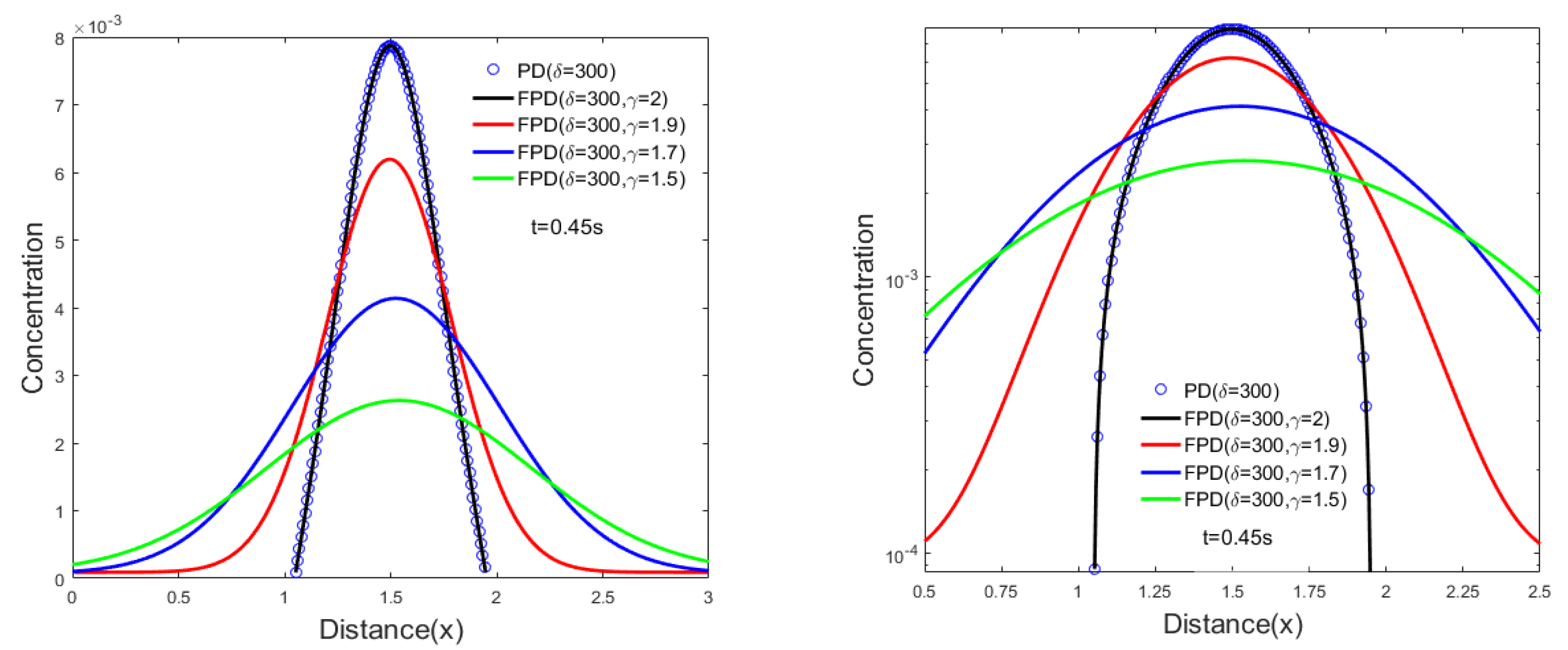
In order to explore the influence of index ($\gamma$) in the FPD model, we calculated the concentration profiles of FPD model with four different orders (Figure 1). The peak value of the FPD model increased with index ($\gamma$). In the super-diffusion, the heavy-tail phenomenon was stronger as index ($\gamma$) decreased. The peak value decreased dramatically. This indicates that the FPD model can characterize the nonlocality of anomalous diffusion. A smaller index ($\gamma$) represents stronger super-diffusion behavior. The numerical results also clearly show that the FPD model reduced to the PD model when the index of FPD model was equal to 1.

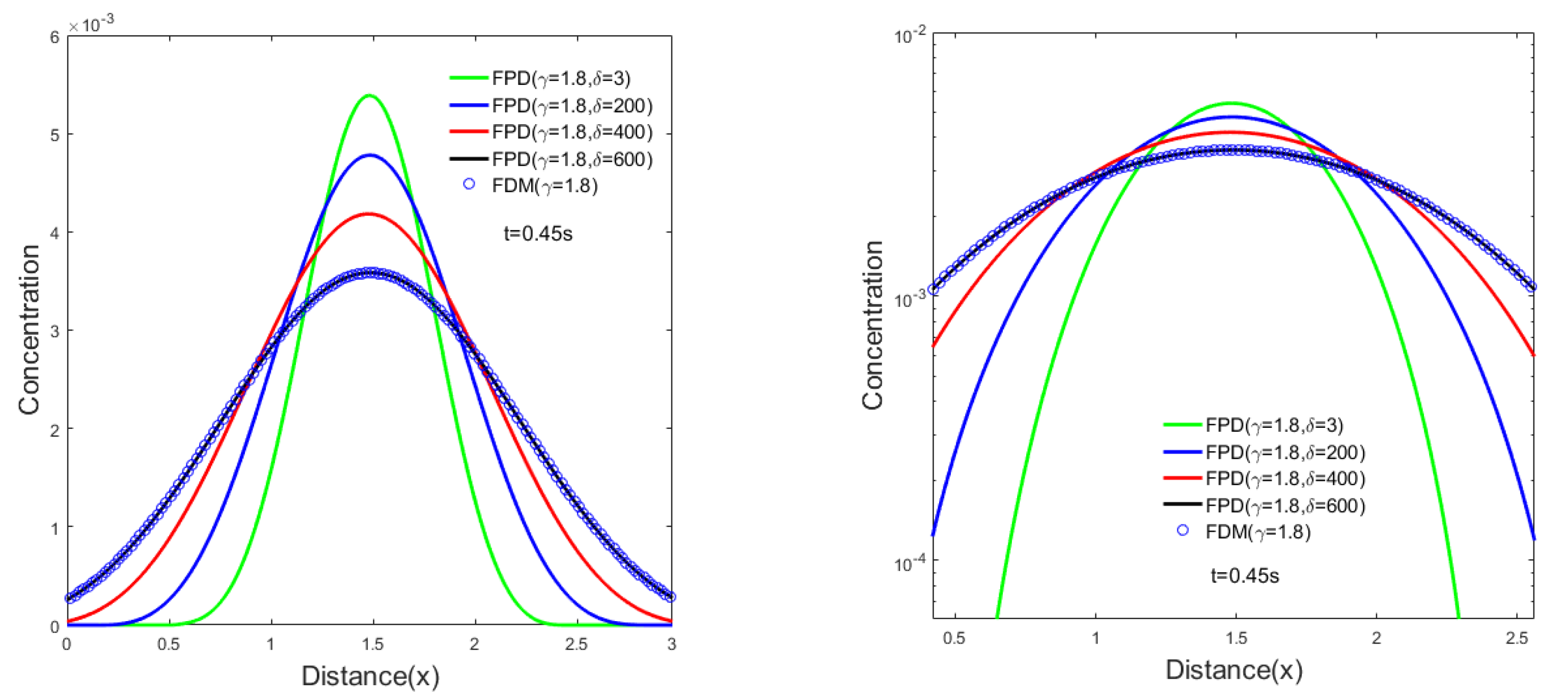
To investigate the effect of near-field range in the FPD model, different sizes of near-field range were used to achieve numerical simulation results of the diffusion processes. It is clear that the peak value of the FPD model decreased with the near-field range, when observing Figure 2. Additionally, heavy-tailing phenomena are present in the numerical results of the FPD model, due to the power-law distribution of jump size characterized by using kernel function. Figure 2 also tells us that the near-field range of the FPD model can determine the degree of spatial nonlocality. It is worth noting that the FPD model is equivalent to the FDM when we use the whole domain as the near-field range in the FPD model. Hence, the index ($\gamma$) together with the size of the near-field range played a critical role in characterizing the nonlocality of the FPD model. Therefore, the nonlocality of physical processes or systems can be more freely described by using the FPD model via introducing index ($\gamma$), and the FDM can be recognized as a special case of the FPD model.

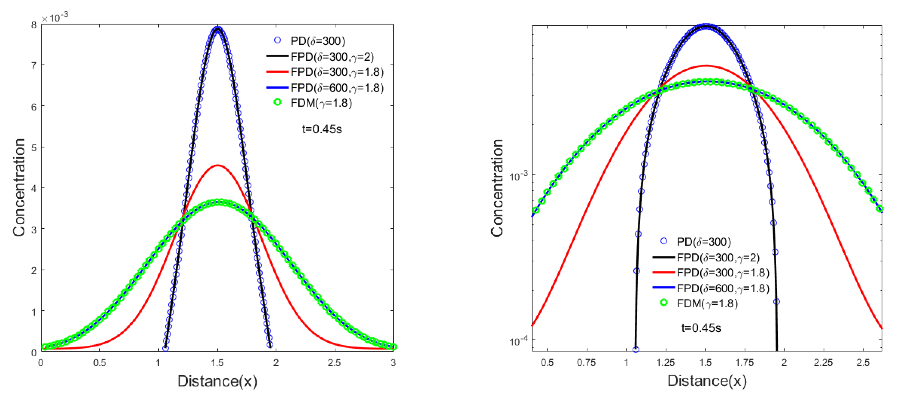
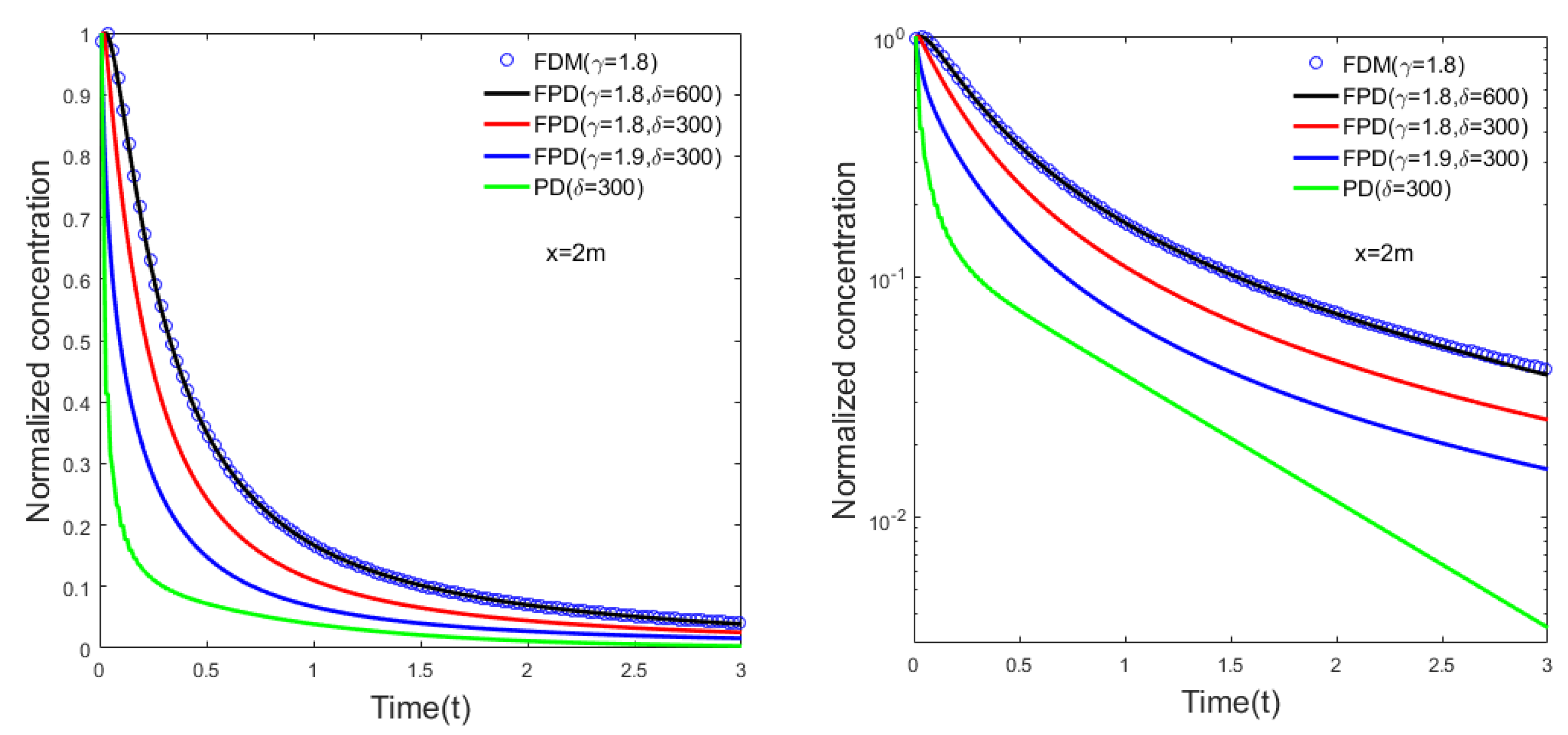
In our numerical simulation, we examined the relationships among the PD model, the FPD model, and the FDM. Two dominant characteristics, the near-source peak and heavy trail phenomenon of spatial nonlocality, are presented in Figure 3. First, our results show that the FPD model is equivalent to the PD model ($\delta =300$, $\gamma =2$) or FDM ($\delta =600$, $\gamma =1.8$). Second, the FPD model involves spatial nonlocality between the PD model and the FDM by adjusting the index ($\gamma$) and near-field range when the other parameters are same. Here we should note that the diffusion behavior of the FPD and PD models approximates to normal diffusion when $\delta =300$ and $\gamma =2$. When $\delta =300$ and $\gamma =1.8$, the FPD model exhibits two main characteristics of anomalous diffusion: (1) a rapidly decreasing peak value for solute concentration; (2) a heavy-tail phenomenon. The FPD model showed the global nonlocality as FDM when $\delta =600$ and $\gamma =1.8$. Therefore, we can conclude that the index ($\gamma$) and the size of the near-field range are crucial factors in characterizing the nonlocality of the FPD model. At last, Figure 4 tells us that the tailing phenomenon in time also existed, which indicates that nonlocality in space leads to a long-range correlation with anomalous diffusion.

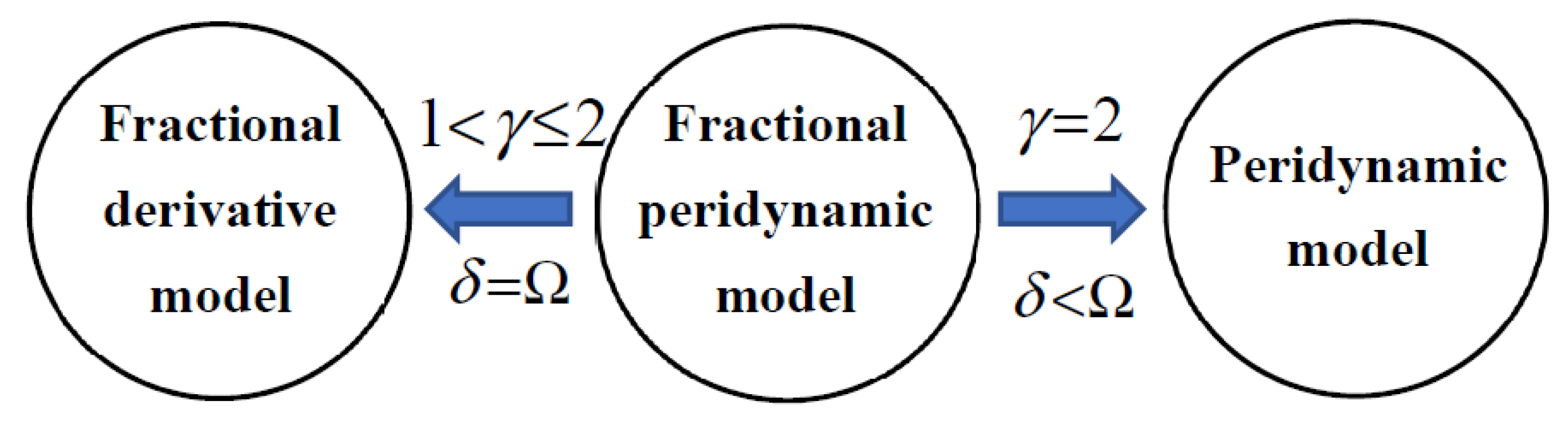
Based on the nonlocal theory, we can establish a connection among the PD model, the FDM, and the FPD model (Figure 5). The FPD model and the PD model are equivalent when $\gamma =2$ for small support areas. Otherwise, the FPD model and FDM are global ones, when $1<\gamma \le 2$ for large areas. It is clear that the FPD model can reduce to the PD model or FDM when choosing different indexes ($\gamma$) and near-field ranges. Thus, FPD model is a generalized nonlocal model.

5. Conclusions

We developed a nonlocal FPD model together with a meshless FPDDO method to solve the anomalous diffusion problem. Our analysis results indicate that the index ($\gamma$) of the power-law kernel function and the size of the near-field range ($\delta$) are critical parameters for describing the different degrees of nonlocality. It is noteworthy that for the indexes $1<\gamma \le 2$ and the near-field range encompassing the whole domain, the FPD model is equal to the FDM. The FPD model reduces to the PD model when the index $\gamma =2$ and the near-field range is small. In short, the FPD model provides a more general strategy for characterizing the nonlocality of physical systems. This model can be extended into 2D and 3D cases to solve nonlocal diffusion problems in multidimensional fields.

References

- Buryachenko, V.A. Generalized effective fields method in peridynamic micromechanics of random structure composites. Int. J. Solids Struct. 2020, 202, 765–786. [Google Scholar] [CrossRef]
- Gur, S.; Sadat, M.R.; Frantziskonis, G.N.; Bringuier, S. The effect of grain-size on fracture of polycrystalline silicon carbide: A multiscale analysis using a molecular dynamics-peridynamics framework. Comput. Mater. Sci. 2019, 159, 341–348. [Google Scholar] [CrossRef]
- Nayak, S.; Ravinder, R.; Krishnan, N.M.A.; Das, S. A peridynamics-based micromechanical modeling approach for random heterogeneous structural materials. Materials 2020, 13, 1298. [Google Scholar] [CrossRef] [PubMed] [Green Version]
- Khan, A.A.; Bukhari, S.R.; Marin, M.; Ellahi, R. Effects of chemical reaction on third-grade MHD fluid flow under the influence of heat and mass transfer with variable reactive index. Heat Transf. Res. 2019, 50, 1061–1080. [Google Scholar] [CrossRef]
- Zhang, Y.; Meerschaert, M.M.; Baeumer, B.; LaBolle, E.M. Modeling mixed retention and early arrivals in multidimensional heterogeneous media using an explicit Lagrangian scheme. Water Resour. Res. 2015, 51, 6311–6337. [Google Scholar] [CrossRef] [Green Version]
- Mortazavi, B.; Rabczuk, T. Multiscale modeling of heat conduction in graphene laminates. Carbon 2015, 85, 1–7. [Google Scholar] [CrossRef] [Green Version]
- Uchida, M.; Kaneko, Y. Nonlocal multiscale modeling of deformation behavior of polycrystalline copper by second-order homogenization method. J. Phys. Condens. Matter 2019, 92, 189. [Google Scholar] [CrossRef]
- Xi, Q.; Fu, Z.J.; Wu, W.J.; Wang, H.; Wang, Y. A novel localized collocation solver based on Trefftz basis for potential-based inverse electromyography. Appl. Math. Comput. 2021, 390, 125604. [Google Scholar] [CrossRef]
- Chen, H.X.; Sun, S.Y. A new physics-preserving IMPES scheme for incompressible and immiscible two-phase flow in heterogeneous porous media. J. Comput. Appl. Math. 2021, 381, 113035. [Google Scholar] [CrossRef]
- You, H.Q.; Yu, Y.; Kamensky, D. An asymptotically compatible formulation for local-to-nonlocal coupling problems without overlapping regions. Comput. Methods Appl. Mech. Eng. 2020, 366, 113038. [Google Scholar] [CrossRef] [Green Version]
- Leng, Y.; Tian, X.C.; Trask, N.A.; Foster, J.T. Asymptotically compatible reproducing kernel collocation and meshfree integration for the peridynamic Navier equation. Comput. Methods Appl. Mech. Eng. 2020, 370, 113264. [Google Scholar] [CrossRef]
- Saeed, T.; Abbas, I.; Marin, M. A GL model on thermo-elastic interaction in a poroelastic material using finite element method. Symmetry 2020, 12, 488. [Google Scholar] [CrossRef] [Green Version]
- Chen, W.; Sun, H.G.; Zhang, X.; Korošak, D. Anomalous diffusion modeling by fractal and fractional derivatives. Comput. Math. Appl. 2010, 59, 1754–1758. [Google Scholar] [CrossRef] [Green Version]
- Qiao, C.T.D.; Xu, Y.; Zhao, W.D.; Qian, J.Z.; Wu, Y.T.; Sun, H.G. Fractional derivative modeling on solute non-fickian transport in a single vertical fracture. Front. Phys. 2020, 8, 378. [Google Scholar] [CrossRef]
- Qiu, L.; Hu, C.; Qin, Q.H. A novel homogenization function method for inverse source problem of nonlinear time-fractional wave equation. Appl. Math. Lett. 2020, 109, 106554. [Google Scholar] [CrossRef]
- Sun, H.G.; Zhang, Y.; Wei, S.; Zhu, J.; Chen, W. A space fractional constitutive equation model for non-Newtonian fluid flow. Commun. Nonlinear Sci. Numer. Simul. 2018, 62, 409–417. [Google Scholar] [CrossRef]
- Sun, H.G.; Chen, W.; Li, C.; Chen, Y.Q. Fractional differential models for anomalous diffusion. Physica A 2010, 389, 2719–2724. [Google Scholar] [CrossRef]
- Brociek, R.; Chmielowska, A.; Slota, D. Parameter Identification in the Two-Dimensional Riesz Space Fractional Diffusion Equation. Fractal Fract. 2020, 4, 39. [Google Scholar] [CrossRef]
- Ganji, R.M.; Jafari, H.; Baleanu, D. A new approach for solving multi variable orders differential equations with Mittag-Leffler kernel. Chaos Solitons Fractals 2020, 130, 109405. [Google Scholar] [CrossRef]
- Chang, A.L.; Sun, H.G. Time-space fractional derivative models for CO2 transport in heterogeneous media. Fract. Calc. Appl. Anal. 2018, 21, 151–173. [Google Scholar] [CrossRef] [Green Version]
- Nikan, O.; Jafari, H.; Golbabai, A. Numerical analysis of the fractional evolution model for heat flow in materials with memory. Alex. Eng. J. 2020, 59, 2627–2637. [Google Scholar] [CrossRef]
- Hu, D.; Cai, W.; Song, Y.; Wang, Y.S. A fourth-order dissipation-preserving algorithm with fast implementation for space fractional nonlinear damped wave equations. Commun. Nonlinear Sci. Numer. Simul. 2020, 91, 105432. [Google Scholar] [CrossRef]
- Rezapour, S.; Mohammadi, H.; Jajarmi, A. A new mathematical model for Zika virus transmission. Adv. Differ. Equ. 2020, 2020, 589. [Google Scholar] [CrossRef]
- Tuan, N.H.; Ganji, R.M.; Jafari, H. A numerical study of fractional rheological models and fractional Newell-Whitehead-Segel equation with non-local and non-singular kernel. Chin. J. Phys. 2020, 68, 308–320. [Google Scholar] [CrossRef]
- Silling, S.A. Reformulation of elasticity theory for discontinuities and long-range forces. J. Mech. Phys. Solids 2000, 48, 175–209. [Google Scholar] [CrossRef] [Green Version]
- Silling, S.A.; Epton, M.; Weckner, O.; Xu, J.; Askari, E. Peridynamic states and constitutive modeling. J. Elast. 2007, 88, 151–184. [Google Scholar] [CrossRef] [Green Version]
- Shojaei, A.; Mossaiby, F.; Zaccariotto, M.; Galvanetto, U. An adaptive multi-grid peridynamic method for dynamic fracture analysis. Int. J. Mech. Sci. 2018, 144, 600–617. [Google Scholar] [CrossRef]
- Wang, J.; Xu, L.; Wang, J. Static and dynamic green’s functions in peridynamics. J. Elast. 2017, 126, 95–125. [Google Scholar] [CrossRef]
- Galvanetto, U.; Sarego, G.; Zaccariotto, M.; Luongo, F. Examples of applications of the peridynamic theory to the solution of static equilibrium problems. Aeronaut. J. 2015, 119, 677–700. [Google Scholar]
- Shojaei, A.; Hermann, A.; Seleson, P.; Cyron, C.J. Dirichlet absorbing boundary conditions for classical and peridynamic diffusion-type models. Comput. Mech. 2020, 66, 773–793. [Google Scholar] [CrossRef]
- Buryachenko, V.A. Variational principles and generalized Hill’s bounds in micromechanics of linear peridynamic random structure composites. Math. Mech. Solids 2020, 25, 682–704. [Google Scholar] [CrossRef]
- Zhang, H.W.; Li, H.; Ye, H.F.; Zheng, Y.G.; Zhang, Y.X. A coupling extended multiscale finite element and peridynamic method for modeling of crack propagation in solids. Acta Mech. 2019, 230, 3667–3692. [Google Scholar] [CrossRef]
- Mengesha, T.; Du, Q. Multiscale analysis of linearized peridynamics. Commun. Math. Sci. 2015, 13, 1193–1218. [Google Scholar] [CrossRef]
- Madenci, E.; Barut, A.; Dorduncu, M. Peridynamic Differential Operator for Numerical Analysis; Springer: Berlin/Heidelberg, Germany, 2019; pp. 14–24. [Google Scholar]
- Gu, X.; Zhang, Q.; Madenci, E. Refined bond-based peridynamics for thermal diffusion. Eng. Comput. 2019, 36, 2557–2587. [Google Scholar] [CrossRef]
- Shojaei, A.; Galvanetto, U.; Rabczuk, T.; Jenabi, A.; Zaccariotto, M. A generalized finite difference method based on the peridynamic differential operator for the solution of problems in bounded and unbounded domains. Comput. Methods Appl. Mech. Eng. 2019, 343, 100–126. [Google Scholar] [CrossRef]
- Khayyer, A.; Gotoh, H.; Falahaty, H.; Shimizu, Y. Towards development of enhanced fully-Lagrangian meshfree computational methods for fluid-structure interaction. J. Hydrodyn. 2018, 30, 49–61. [Google Scholar] [CrossRef]
- Bazazzadeh, S.; Shojaei, A.; Zaccariotto, M.; Galvanetto, U. Application of the peridynamic differential operator to the solution of sloshing problems in tanks. Eng. Comput. 2019, 36, 45–83. [Google Scholar] [CrossRef]
- Gerstle, W.; Silling, S.; Read, D.; Tewary, V.; Lehoucq, R. Peridynamic simulation of electromigration. Comput. Mater. Contin. 2008, 8, 75–92. [Google Scholar]
- Martowicz, A.; Bryła, J.; Staszewski, W.J.; Ruzzene, M.; Uhl, T. Nonlocal elasticity in shape memory alloys modeled using peridynamics for solving dynamic problems. Nonlinear Dyn. 2019, 97, 1911–1935. [Google Scholar] [CrossRef] [Green Version]
- Jiang, X.; Xu, M.; Qi, H. The fractional diffusion model with an absorption term and modified Fick’s law for non-local transport processes. Nonlinear Anal. Real World Appl. 2010, 11, 262–269. [Google Scholar] [CrossRef]
- Rabei, E.M.; Almayteh, I.; Muslih, S.; Baleanu, D. Frctional, Hamilton-Jacobi formulation of system within Caputo’s factional derivative. Phys. Scr. 2008, 77, 015101. [Google Scholar] [CrossRef]
- Madenci, E.; Oterkus, E. Peridynamic Theory and Its Applications; Springer: Berlin/Heidelberg, Germany, 2014; pp. 24–25. [Google Scholar]
- Lakshmikantham, V.; Vatsala, A.S. Theory of fractional differential equations. Nonlinear Anal. 2008, 69, 2677–2682. [Google Scholar] [CrossRef]
- Zhang, Y.; Benson, D.A.; Reeves, D.M. Time and space nonlocalities underlying fractional-derivative models: Distinction and literature review of field applications. Adv. Water Resour. 2009, 32, 561–581. [Google Scholar] [CrossRef]
Figure 1.
The concentration profiles using the peridynamic (PD) model and the fractional peridynamic (FPD) model with near-field range at four different space fractional indexes: , , , and . Other model parameters were , , and . The right plot is the semi−log form.
Figure 2.
The concentration profiles using the FDM with space fractional index and the FPD model with space index at four near-fields ranges : , , , and . Other model parameters were , , and . The right plot is the semi−log form.
Figure 3.
The concentration profiles of the PD model with near-field range , the FDM with space fractional index , and the FPD model at different space indexes and near-field ranges: , ; , ; , . Other model parameters were , , and . The right plot is the semi−log form.
Figure 4.
The normalized concentration profiles of PD with near-fields range , the FDM with space fractional index , and the FPD models with different indexes and near-field ranges: , ; , ; , . Other model parameters were , , and . The right plot is the semi−log form.
Figure 5.
The relationship among three models (PD model, FPD model, and FDM).
Publisher’s Note: MDPI stays neutral with regard to jurisdictional claims in published maps and institutional affiliations. |
© 2021 by the authors. Licensee MDPI, Basel, Switzerland. This article is an open access article distributed under the terms and conditions of the Creative Commons Attribution (CC BY) license (https://creativecommons.org/licenses/by/4.0/).
Share and Cite
MDPI and ACS Style
Wang, Y.; Sun, H.; Fan, S.; Gu, Y.; Yu, X. A Nonlocal Fractional Peridynamic Diffusion Model. Fractal Fract. 2021, 5, 76. https://0-doi-org.brum.beds.ac.uk/10.3390/fractalfract5030076
AMA Style
Wang Y, Sun H, Fan S, Gu Y, Yu X. A Nonlocal Fractional Peridynamic Diffusion Model. Fractal and Fractional. 2021; 5(3):76. https://0-doi-org.brum.beds.ac.uk/10.3390/fractalfract5030076
Chicago/Turabian StyleWang, Yuanyuan, HongGuang Sun, Siyuan Fan, Yan Gu, and Xiangnan Yu. 2021. "A Nonlocal Fractional Peridynamic Diffusion Model" Fractal and Fractional 5, no. 3: 76. https://0-doi-org.brum.beds.ac.uk/10.3390/fractalfract5030076