
The Fractal Tapestry of Life: III Multifractals Entail the Fractional Calculus


1
Office of Research and Innovation, North Carolina State University, Rayleigh, NC 27695, USA
2
Center for Nonliner Science, University of North Texas, Denton, TX 76203, USA
Fractal Fract. 2022, 6(4), 225; https://0-doi-org.brum.beds.ac.uk/10.3390/fractalfract6040225
Submission received: 10 March 2022
/
Revised: 29 March 2022
/
Accepted: 12 April 2022
/
Published: 15 April 2022
(This article belongs to the Special Issue Operators of Fractional Calculus and Their Multidisciplinary Applications)
Abstract
:This is the third essay advocating the use the (non-integer) fractional calculus (FC) to capture the dynamics of complex networks in the twilight of the Newtonian era. Herein, the focus is on drawing a distinction between networks described by monfractal time series extensively discussed in the prequels and how they differ in function from multifractal time series, using physiological phenomena as exemplars. In prequel II, the network effect was introduced to explain how the collective dynamics of a complex network can transform a many-body non-linear dynamical system modeled using the integer calculus (IC) into a single-body fractional stochastic rate equation. Note that these essays are about biomedical phenomena that have historically been improperly modeled using the IC and how fractional calculus (FC) models better explain experimental results. This essay presents the biomedical entailment of the FC, but it is not a mathematical discussion in the sense that we are not concerned with the formal infrastucture, which is cited, but we are concerned with what that infrastructure entails. For example, the health of a physiologic network is characterized by the width of the multifractal spectrum associated with its time series, and which becomes narrower with the onset of certain pathologies. Physiologic time series that have explicitly related pathology to a narrowing of multifractal time series include but are not limited to heart rate variability (HRV), stride rate variability (SRV) and breath rate variability (BRV). The efficiency of the transfer of information due to the interaction between two such complex networks is determined by their relative spectral width, with information being transferred from the network with the broader to that with the narrower width. A fractional-order differential equation, whose order is random, is shown to generate a multifractal time series, thereby providing a FC model of the information exchange between complex networks. This equivalence between random fractional derivatives and multifractality has not received the recognition in the bioapplications literature we believe it warrants.
1. Introduction
In [1], it was argued that Sir Isaac Newton transformed Natural Philosophy into today’s Science by explaining that motion is at the core of mechanics and describing the manner in which the planets orbit the sun using the inverse power law (IPL) of gravity. He described a planet’s trajectory using geometry, which was the contemporary mathematical language of scientific discourse and had been for over a millennium. Fluxions, his version of the differential calculus, were not mentioned in the Principia wherein he revealed his new vision of the universe. The lack of discussion of differentials is curious since that would have been the more natural way to create the orbits, as every college freshman learns today in their Introductory Physics course. However, a handful of contemporary mathematicians did recognize in a number of his more involved geometrical arguments that he clearly had the differential calculus in the back of his mind. A careful reading of his text makes this evident from our three-hundred-year-plus vantage point on the matter.
What Newton accomplished was to reveal what was entailed by fluxions (the deferential calculus) without explicitly referring to it; and in that way, he convinced generations of scientists of the value of analyzing how physical phenomena change in space and over time. Whether by serendipity or conscious plan, it is not clear which, Newton forged a path for less gifted investigators to follow and contribute to the nascent scientific discipline of mechanics and to physics generally. He enabled the more adventurous to step beyond the safeguards of geometry during that time of transition into the new and more encompassing world of the differential. It was speculated in prequel I that we have reached another epoch of transition [2]:
…it has occurred to a number of the more philosophically attuned contemporary scientists that we are now at another point of transition, where the implications of complexity, memory, and uncertainty have revealed themselves to be barriers to our future understanding of our technological society. The fractional calculus (FC) has emerged from the shadows as a way of taming these three disrupters with a methodology capable of analytically smoothing their singular natures.
Looking back over the past two centuries, it is evident that the view of how the human body operates paralleled our growth in understanding of how the physical universe operates as well as how our technological society came into being. This perspective was developed, in large part, using physical analogs and the adaptation of physical principles in some cases without the empirical evidence needed for its justification. Consider homeostasis, thought by many to be a guiding principle of medicine, and to be the biomedical consequence of Le Chattier’s Principle [3]. From this perspective, every human body is believed to have multiple automatic inhibitory mechanisms that suppress disquieting influences, whether those disruptions are generated by the environment external to the body or by malfunctioning internal systems. This particular notion has recently been replaced by homeodynamics, with the recognition that life is a non-equilibrium process and therefore requires rich dynamics to maintain stability [3,4].
Healthy physiologic networks give rise to erratic time series whose fluctuations contain the control information that guide the behavior of these complex networks. It is the statistics of physiological fluctuations that determine the spatial properties of the tree-like structures of the human lung, arterial and venous systems, and other ramified structures [5]. Statistical fractals [6,7] determine the probability density function (PDF) of time intervals in the beating human heart [2,8,9,10], in respiration [11,12,13,14], synchronous response to a metronome [15], in human locomotion [16,17,18,19], in the human nevous sysem [20], in the dynamics of the brain [21,22,23,24], in the walking rehabilitation of the elderly [25,26], motor control [27,28], and interpersonal coordination [29,30], and in human cognition [31].
It is not only fractal statistics that determine the behavior of physiologic networks but fractal dynamics [32] as well. For example, such behavior is found in the firing of certain neurons [22,33,34], as well as in the time series of posture control [35], which determine the dynamic properties of physiologic networks having a large number of characteristic time scales. These and other fractal physiology processes have been the focus of interdisciplinary research on complex networks for more than a decade; see [2,36,37,38].
The scaling of a dynamic network determines whether it is sufficiently complex to be able to efficiently carry out its function. In 2008, West et al. [39] determined preliminary conditions under which information is efficiently exchanged between complex dynamic networks under the rubric of the Principle of Complexity Matching (PCM), which subsequently was absorbed into the more general Principle of Complexity Management [40,41]. This latter principle has been shown to be operative in the flow of blood between the heart and brain [42], in the transmission of oxygen between the lungs and the heart [43], and in the more ephemeral transfer of information during rehabilitation of the elderly [26,28].
In addition, there are vast numbers of other phenomena that, due to their complexity, require increasingly complicated use of the integer calculus (IC) that has served us so well over the past three hundred years in describing the macroscopic world. Newton’s derivation of celestial orbits using geometry was shown to be an unnecessarily restrictive way to think about the phenomena being investigated and it turned out that the IC entered the thinking of most scientists via the back door, so to speak. In fact, it was by means of an entirely different mathematical concept, the fractal, that the non-integer calculus, which we herein refer to as the fractional calculus (FC) gained its present degree of popularity, if not acceptance, in the scientific community.
2. Fractality
Mandelbrot did much more than introduce a new mathematical concept into the scientific lexicon with his notion of fractals [6,44]. He pointed out the obvious and asked why scientists were not modeling the world the way it actually presents itself; much as the boy asked about the emperor’s new clothes in the fairy tale. As Mandelbrot noted, fractals come in three flavors: geometric, statistical and dynamic. Here, we do not dwell on the mathematical properties of each of these kinds of fractals, but instead focus on the statistical properties of experimental datasets and how their fractal nature may be determined and characterized.
As Bogdan et al. [45] emphasize in their brilliant editorial, the understanding of complexity is a fundamental problem in biology, physiology and medicine. Complexity enters into the discussion in a number of ways, including but not limited to multicomponent regulatory mechanisms, where efficient homeostatic control is maintained by means of non-linear feedback loops and disruptive pathologies are brought back into balance by means of homeodynamic control. This notion of homeodynamics offered a radically new concept departing from the traditional homeostatic idea that emphasizes the stability of the internal dynamics with respect to perturbation. Indeed, Lloyd et al. [4] argue in their review that biological systems are homeodynamic as a manifestation of a network’s ability to self-organize at behavior bifurcation points where they lose stability and restabilize in a new state. As a result of this self-organization, living systems displays complex behaviors with a spectrum of emergent characteristics, including bistable switches, thresholds, mutual entrainment, and periodic as well as chaotic behavior. These processes may proceed on different spatial and/or time scales, from very rapid processes on the molecular level to the enormously long time scales of evolutionary change. It is such dynamic organization under homeodynamic conditions that make possible the organized complexity of life.
Herein, we focus on the generic notion of fractality to facilitate our understanding of complexity in the life sciences [32,37,46,47,48] and its ultimate entailment of the FC, see [49] for an excellent introduction to bioengineering.
2.1. Fractal Time Series
Random fractals may at first sight appear strange, but fractal statistics have been shown to appear in all manner of familiar phenomena in physical, social and life sciences once they were revealed by Mandelbrot. One property of interest is long-time memory, which can be measured by an autocorrelation function. The proposal of Mandelbrot and van Ness [44], subsequently named fractional Brownian motion (FBM) by Mandelbrot [6], is not compatible with the traditional equilibrium statistical mechanics [50,51]. In FBM, the stationary correlation function of the noise , with a very short correlation time for ordinary diffusion, is replaced by a correlation function , which is still stationary, but not integrable, with a diverging correlation time. The solution to the rate equation for free diffusion with vanishing initial conditions is used to relate the autocorrelation functions:
where the normalized stationary autocorrelation for the noise is defined by
With a proper choice of autocorrelation function, setting and sending t, and to infinity has the effect [52] of reducing Equation (1) for the correlation index to the FBM form [6]:
where the symbol H was adopted by Mandelbrot to denote the scaling first implemented by Hurst [53].
Feder [50] emphasizes, for , the correlation of past and future increments of the time series vanish for all t, thereby yielding an uncorrelated random process. However, for , the process is persistent, indicating that an increasing trend in the past entails an increasing trend in the future for all . Similarly, for , the process is anti-persistent, indicating that an increasing (decreasing) trend in the past entails that a decreasing (increasing) trend in the future is more probable.
Note that the autocorrelation function given for FBM is in direct conflict with what is normally assumed or can be proven from the statistical records of physical networks. Thermal equilibrium requires that events correlated when separated in time by become uncorrelated in the limit which is certainly not the case above. Moreover, in a second-order phase transition, e.g., as the critical point of a fluid is approached from above the fluid density, autocorrelation function transitions from being an exponential with independent increments to being an inverse power law (IPL) with a long-time correlation [54].
The correlation index defined by Equation (3) is expressed in terms of the correlation dimension and is the dimension of an uncorrelated random process for which as seen in Brownian motion. On the other hand, a regular one-dimensional curve has , corresponding to a completely correlated process with . A fractal time series , in general, satisfies the homogeneous scaling relation:
and generates another fractal process with the same statistics and typically . As the size of a network increases, it provides increasing opportunity for variability, which is necessary in order to maintain stability. Scaling provides a measure of complexity in dynamic networks, indicating that the network’s observables can simultaneously fluctuate over many time and/or space scales.
The FBM process proposed by Mandelbrot and van Ness [44] lies between Brownian motion and white noise. In both cases, the continuum is characterized by the homogenous scaling law given by Equation (4) but in the frequency domain [44]:
which is the power spectrum for a fractal process. The statistics for Brownian motion are Gaussian and the spectral scaling index is , since . Similarly, the statistics for white noise are Gaussian as well but with a flat spectrum such that . The situation with is the well-known situation of 1/f noise [55,56] which has been empirically determined in a large number of natural and physical phenomena as recorded in the excellent review article by Deligniéres and Marmelat [57] on the connections between fractal fluctuations and complexity.
Scaling PDF: The hallmarks of fractal statistics are spatial (x) inhomogeneity, temporal (t) intermittency and the phase space trajectory () exchanged for the dynamic variable . In phase space, the scaling of the dynamic variable is replaced by a scaling of the PDF :
as we subsequently show for quite general complex phenomena. There is a broad class of PDFs for which the functional form of is left unspecified. It is straightforward to calculate the average value of using the PDF given by Equation (6):
and the overall constant is determined by the scaling variable averaged over the PDF :
Notice that using the scaling PDF that it is the average of the dynamic variable that now manifests the scaling property:
For FBM, it is clear that the scaling parameter is given by and the PDF given by is Gaussian, which is not the situation in general. The more general case is only constrained by the complexity of the network through the scaling behavior of the moments of the PDF.
2.2. Multifractal Time Series
One property that stands out from the multiple studies performed on the information transfer between complex dynamic physiologic networks is that such living networks exist at, or are on the edge of, a phase transition [58,59]. Such network configurations optimize both intra- and inter-network information transmission [39]. Moreover, the generic statistical distribution that characterizes a diverse collection of complex networks is the IPL, whether modeling the connectivity of the internet or social groups [60], the frequency or magnitude of earthquakes [61], the number of solar flares, the time intervals in conversational turn taking [62], and many other phenomena; see, for example, [63,64,65] for reviews of exemplars and the discussion of mathematics.
As pointed out by West and Grigolini [7], 1/f noise is not strictly speaking noise, since noise by definition does not carry useful information about network dynamics. The IPL index of a 1/f spectrum is the temporal signature of the self-similarity property of a critical dynamic state. Bak [66] proposed the first theory of critical behavior that is independent of an external control parameter such as temperature, in which a network’s internal dynamic attracts the network elements into a critical state [67]. This attraction is called self-organized criticality (SOC) and the associated 1/f variability occurs in catastrophic phenomena such as brainquakes [22,33,68,69], spral waves in astrocyte syncytia [70], earthquakes, the highly optimized tolerant (HOT) theory of forest fires [64,71] and punctuated equilibria [57]. Finally, there exists a connection between neural organization and information theory, the empirical laws of perception [72], and the production of 1/f noise [73], with the remarkable property that 1/f signals are encoded and transmitted by sensory neurons more efficiently than are white noise signals [74].
The signature of SOC is the IPL index of the 1/f spectrum of the time intervals between critical events, with an IPL waiting-time PDF, a property historically referred to as temporal complexity. We therefore refer to this form of SOC as self-organized temporal criticality (SOTC) and identify the critical events as crucial [7,75]. The 1/f variability IPL index and that of the underlying time series statistics are related and taken to be measures of the network complexity and the relation to multifractality is emphsized by Mandelbrot [63].
We closed prequel II [76] with a brief discussion of multifractals along with a promise to expand on its overlap with the FC. These earlier comments began with the observation of the need to replace the historical engineering paradigm of ‘signal-plus-noise’ with a model of biomedical time series having fractal statistics. The scaling behavior of such biomedical time series entails the fact that no single scale or frequency carries the signal, but rather pieces of the signal are distributed across a spectrum of scales. However, even this generalization of the engineering paradigm was shown to be too restrictive to properly describe the richness of physiologic time series. A number of physiologic time series were found to be characterized by a distribution of scaling parameters and therefore to belong to a broader class of complex processes known as multifractals. Such multifractal time series appear in the rich variability of healthy physiological networks, including but not restricted to human gait [32], cerebral blood flow (CBF) [77,78] and heart rate variability (HRV) [79,80,81], and changes in scaling behavior [82] reflect certain kinds of pathologies, as discussed in prequel I [2] of this series.
There are many fractal time series generated by multiple processes having long-term memory of the underlying dynamic networks, with FBM being only one exemplar. For example, physiological signals, such as cerebral blood flow (CBF), are typically generated by complex self-regulatory networks that handle inputs with a spectrum of characteristics. The importance of this self-regulation was recognized by Ivanov et al. [81], who determined that time series for healthy human HRV, rather than being fractal, are multifractal, which is to say that the time series are not restricted to a single fractal but described by a spectrum of fractal dimensions. They also uncovered the fact that a narrowing of the multifractal spectrum is diagnostic of congestive heart failure as well as other cardiac pathologies [83]. It is noteworthy that multifractals are defined by time series with spectra of fractal dimensions (scaling exponents). Such an effect arises due to the scaling index changing over time—see, e.g., Feder [50]—resulting in the underlying process being characterized by a spectrum of fractal dimensions, or scaling parameters. West et al. [78] similarly determined that CBF in healthy humans is also multifractal, and showed that CBF time series have a broad uni-modal multifractal spectrum and the width of this spectrum is greatly reduced for people who suffer from ”severe” migraines.
In [76], it was pointed out that multifractals are made up of many interwoven subsets with different local scaling exponents. The statistical properties of these subsets are characterized by the spectral distribution of fractal dimensions as depicted therein in Figure 11. In that figure, we fit the multifractal spectrum for the middle CBF velocity time series for a healthy control group using the solution to a linear Langevin equation [78], compared with a group of migraineurs. The width of the multifractal distribution centered on the local scaling exponent for the CBF velocity for the migraineurs is constricted by a factor of three over that of the control group, suggesting that the underlying process has lost a great deal of flexibility. The physiological advantage of multifractal processes is that they are highly adaptive, so that the brains of healthy individuals readily adapt to the multifractality of the interbeat interval time series [84,85].
Multifractal signal processing: Mandelbrot was the first to recognize that signals that are singular at almost every point, fractal signals, are typical of physiological datasets. So how do we interpret a multifractal signal, or a fractal signal for that matter? A long-standing strategy for interpreting a signal is to construct the Fourier transform applied to an experimental time series. Although the method is mathematically unassailable, the utility of the various derived quantities has been questioned. The basis for these queries is the mutually exclusive treatment of time and frequency in the specification of the signal, that is, the time series is assumed to be infinitely long and each frequency is defined for a monochromatic infinitely long wave train. However, all time series in medicine are of finite duration and dominant frequencies change over time. The recognition of this limitation of the (time, frequency) representation of Fourier signals lead to the development of the wavelet transform method for representing one-dimensional signals as a function of time and frequency; see, e.g., [86].
One can develop the mathematical infrastructure for analyzing the properties of multifractals following the wavelet-transform modulus-maxima method (WTMM) laid out by Mallat [86] or by adopting the more intuitive box counting techniques used by Feder [50]. The singularity spectrum can be calculated from the WTMM [86,87,88] at each data point in the time series. Given the time series and the WTMM time series at a scale l denoted by , the partition function can be expressed in terms of the qth moment:
where is the position of the local maxima of the transformed dataset at the fixed scale . The quantity is the mass exponent and is related to the generalized dimension where the fractal dimension is the information dimension is and the correlation dimension is . Measurements of the and the spectrum of singularities provide global and statistical information of the scaling properties of fractal measures. This information is similar to the power spectral density obtained from the Fourier transform of a time series that quantifies the relative contributions of the underlying frequencies. The spectral function quantifies the relative contribution of the underlying singularities. However, just as the Fourier transform does not keep track of the time-ordering of the frequencies contributing to a power spectral density, neither does denote the temporal locations of the singularities.
An important consequence of this analysis is that the Hölder exponent will not be constant, if and only if, large fluctuations scale differently from small fluctuations. The multifractal spectrum describes how the local fractal exponents h contribute to a multifractal time series. We note that h and f are independent variables, as are q and . These two sets of variables are interrelated by the general formalism of Legrendre transform pairs:
using the sign convention of Feder [50]. The local fractal exponent h varies with the q-dependent Hölder exponent through:
The singularity spectrum given by Equation (11) can therefore be written:
where both the mass exponent and its derivative are determined using WTMM on the dataset. Thus, a multifractal spectrum can only give an indication of the span of dimensions being accessed by the dynamic process and not the order in time at which they occur.
A vast literature has become available on multifractals and their processing techniques over the last quarter century, including the brain–heart connection [9,42,43,89,90], the behavioral experiments on syncopated finger tapping [27,28,91,92], dyadic conversation [62] and information flow through different parts of the brain [12,36,93]. The current research work on extended cognition, a recent theory in which mental processes are hypothesized to extend beyond the brain and incorporate interactions with the environment in which it is embedded [94,95], is entailed by the information transferred between complex networks, such as the environment and the brain.
Our goal is to compare the multifractal spectra of a complex network perturbed by another complex network as a function of their respective IPL indices, as in [41], since the IPL indices are the proposed measures of complexity. A stable procedure to generate the singularity spectrum from the events of the complex networks is needed. A number of such procedures have been proposed, but only one of which has proven satisfactory for non-ergodic networks and which we now discuss.
2.2.1. Ergodicity Breaking
Piccinini et al. [96] generate a single time series using an IPL PDF, which is then used to construct a multifractal spectrum equivalent to creating a Lévy process. This construction creates an apparent contradiction, since using the generalized central limit theorem it is possible to conclude that Lévy processes are monofractal, with the fractal dimension being related to the Lévy index [97]. Why, then, does the algorithm [98] used produce wide parabolas when applied to this time series, since such a parabola is a clear indication of multifractality? As they explain, the reason is that the constant fractal exponent resulting from the generalized central limit theorem is tied to the fact that averages are carried out using ensemble PDFs, whereas the procedure used by Piccinini et al. [96] evaluates averages using a single time series. Consequently, if the time series is non-ergodic, the two kinds of averages can be very different [41].
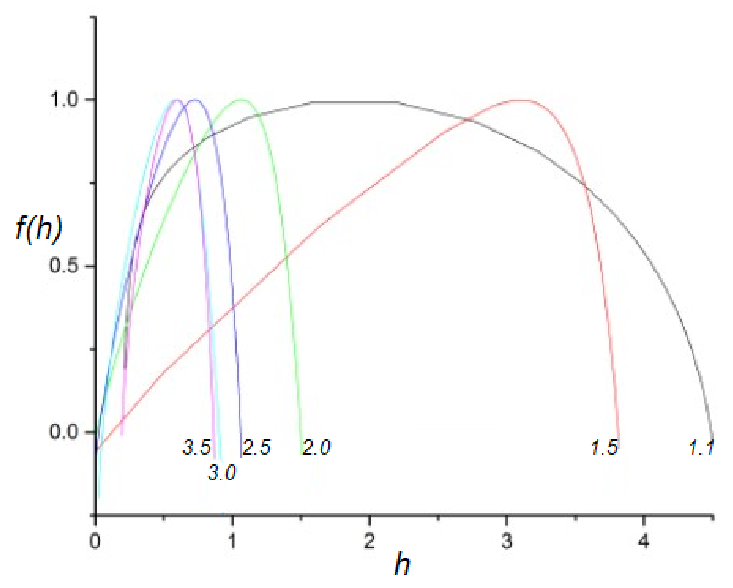
Let us plot the multifractal spectra obtained for time series generated using various IPL indices . As shown in Figure 1, the spectrum for is very broad, while the spectrum for is still broad, but with significantly less weight in the tails. As expected, when is further increased, the generated spectra become narrower, their peaks shift towards , and the networks they represent deviate less and less from being ergodic with an increasing IPL index. Thus, this figure compliments the IPL index as a representation of the complexity of a dynamic time series series by explicitly showing the width of the multifractal spectrum.
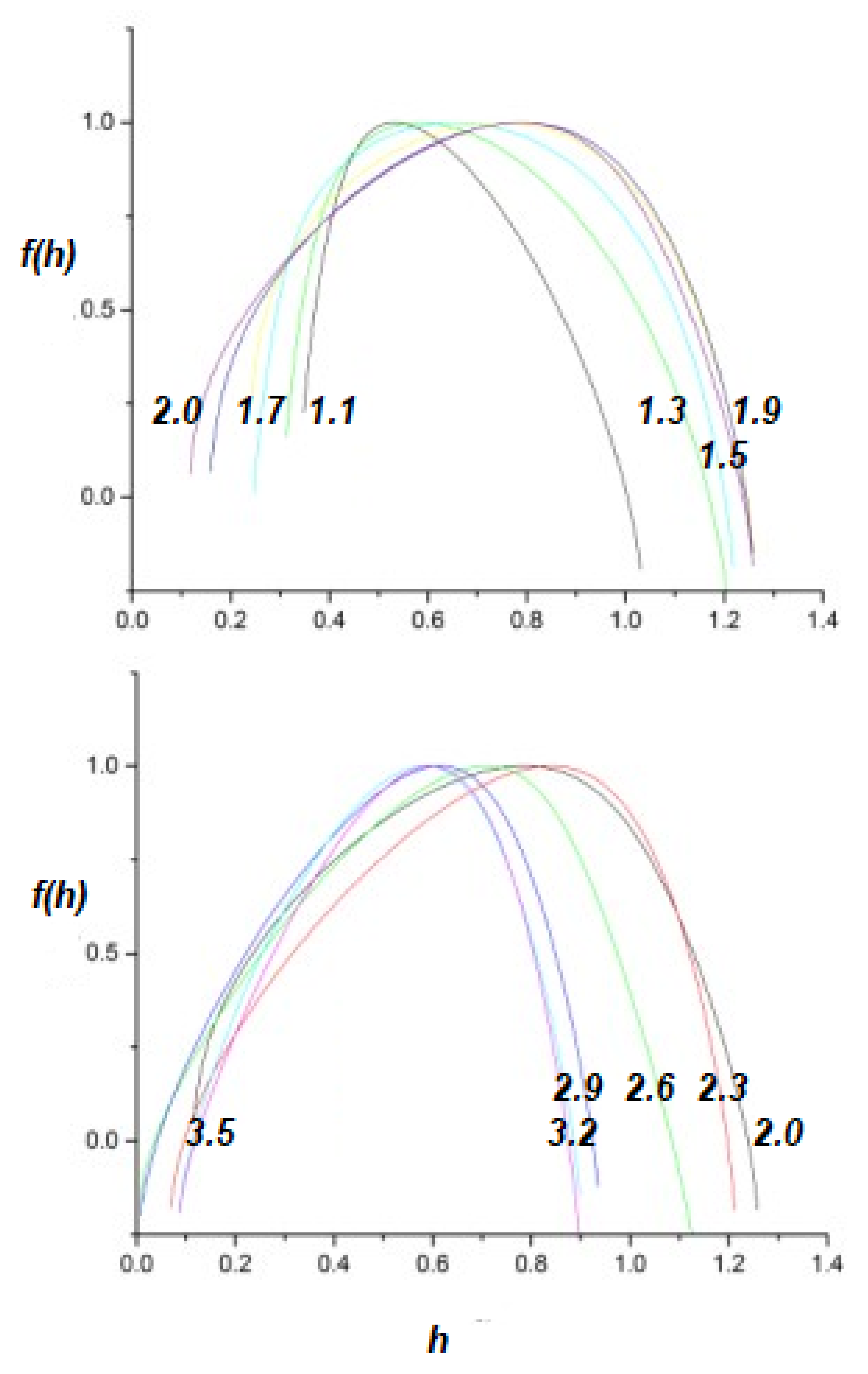
Introducing a truncation into the IPL waiting-time PDF has a dramatic effect, as can be seen in Figure 2. While networks with , which have a finite first moment, are essentially unaffected by truncation, networks with , whose first moment diverges, behave differently than they did without truncation. The smaller the IPL index , the more the parabola is shifted to a smaller scaling index h and becomes more sharply peaked at approximately . The reason for this change becomes clear when we stop and consider that the truncation mainly affects networks that have longer tails (). More significantly, truncating a PDF affects the scaling of the large fluctuations (since the tail of the distribution is suppressed) and leaves the scaling of the small fluctuations unaffected. Thus, the multifractal properties of these networks are substantially altered by truncation. When , the average length of the laminar regions between critical events would diverge when unaltered, but the truncation prevents it from doing so, which attracts the peak of the singularity spectrum to a value closer to .
2.2.2. Information Transfer
The newly emerging fields of network physiology and network medicine [99,100,101] have stimulated research that spans the gap between microbiology and neurophysiology, and has benefited from the significant advances recently made in the field of dynamic complex networks. One of the more significant advances in these new fields of research is understanding the efficiency of the transport of information from one complex network to another, during their interaction. We show that the transport of information from one dynamic complex network to another is equivalent to the transmission of the multifractality property. This information transport is captured by the PCM, which relies on the roles played by criticality [102] and ergodicity breaking in the network dynamics [37]. Moreover, as subsequently pointed out by Mahmoodi et al. [103], the PCM is consistent with the notion of transporting global properties from one complex network to another. This mechanism has also been called 1/f resonance to denote the increase in information transfer associated with the enhanced increase in information transfer efficiency between networks associated with a single frequency and that associated with the matching of IPL indices of the interacting networks [40].
The organ–organ interaction perspective of the new network physiology enriches the therapeutic culture, with the infusion of basic concepts such as comorbidity being a manifestation of different diseases being interconnected [104]. The degree and fidelity of a network’s response are a consequence of both the average h and the width of the singularity spectrum of the perturber relative to the responder. The communication between two complex networks is frequently interpreted [27,28,62], following West et al. [39,40,105], to be a manifestation of complexity matching and consequently of the information exchange being facilitated when the interacting networks share the same dynamical complexity as measured by the IPL index of the PDF for the time interval between crucial events. In turn, the IPL index is related to the fractal dimension of the underlying stochastic process. The signature of the shared dynamical complexity is multifractality [106,107], namely the dynamic processes having the same range of values of fractal dimensions, or equivalently, comparable spectra of IPL indices, activated by the emergence itself of cognition [108,109,110,111,112].
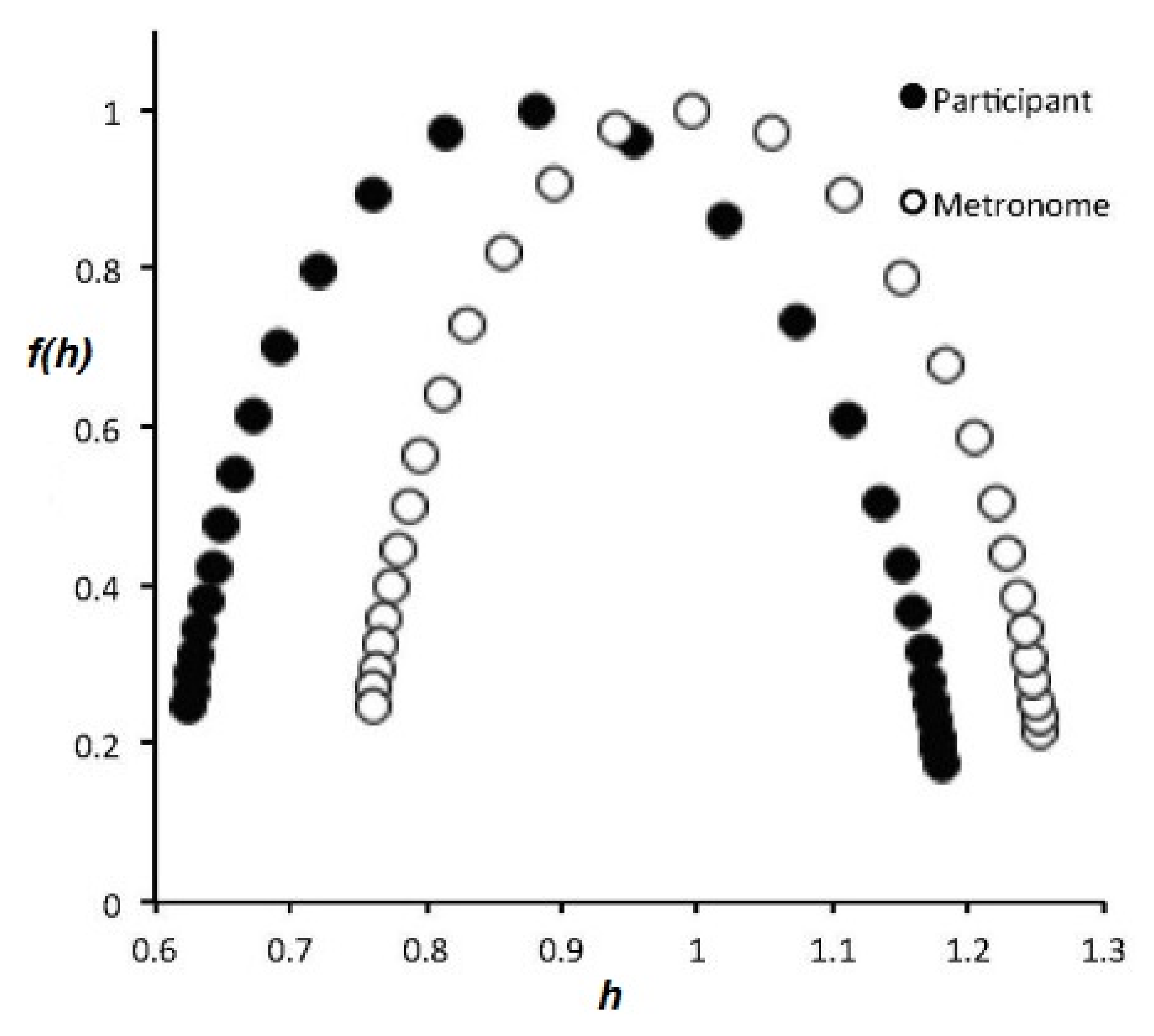
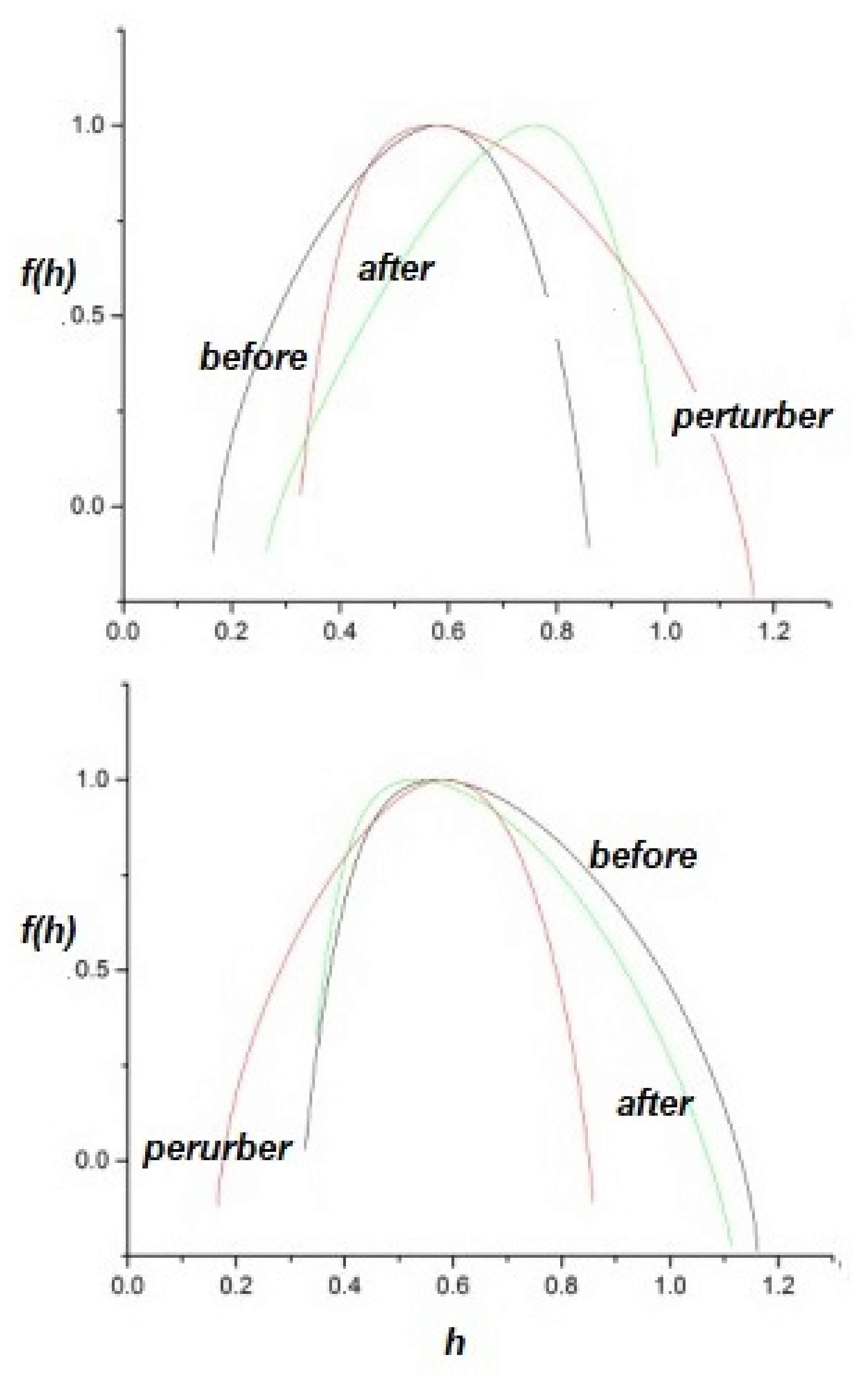
One way to visualize the multifractal spectrum that has been used extensively herein is by means of the singularity spectrum . The broader the parabola, the more multifractal a network, in the sense that more values of fractal dimensions contribute to the variability of the time series. A very narrow parabola centered on h = 0.5 indicates an essentially monofractal ergodic system. This interpretation is confirmed by experimental results [113] based on the transfer of global properties from one complex network to another. In these latter experiments, a multifractal metronome generates a spectrum of fractal dimensions as a function of the excitatory signal and it is this multifractal spectrum that is captured by the brain-response stimulation. As noted in prequel I, the multifractal behavior depicted by the uni-modal spectrum provides a unique measure of complexity of the underlying network. It is worth noting further that the same displacement of the metronome spectrum, from the body response spectrum, is observed for walking in response to a multifractal metronome, as depicted in Figure 3.
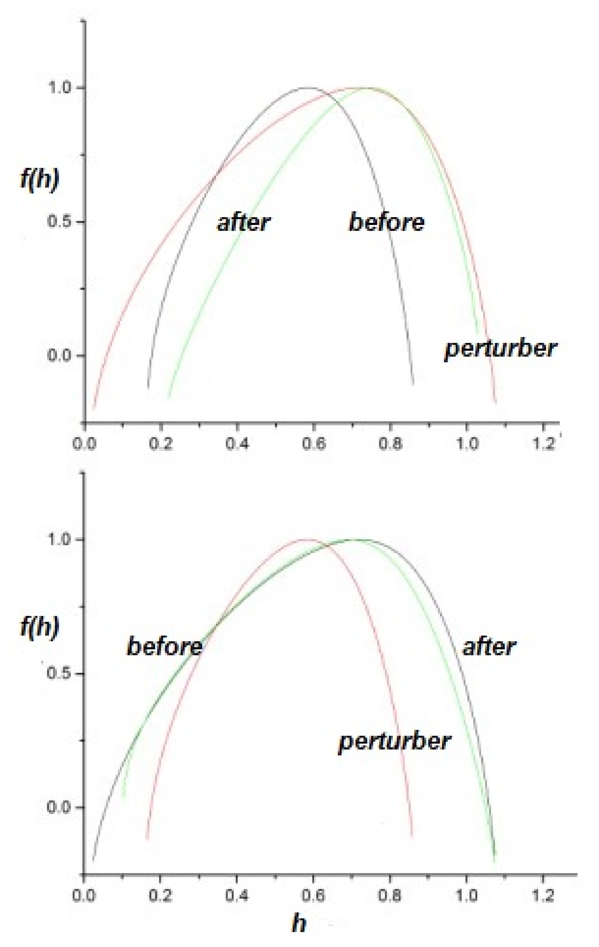
To perturb the multifractal spectrum of a complex network, consider a complex network P perturbing a responsive complex network R, with appropriately indexed parameters. The upper panel of Figure 4 depicts the response of a network with to a perturbing network having . The inverted parabola of the responding network becomes broader in this case and shifts to increasing h, so the perturbed network becomes more multifractal and less ergodic than it was before being perturbed. This result is not unexpected, since the response of the perturbed network is high for these values of the IPL indices, . One can interpret this result as the responding network acquiring certain of the characteristics of the perturbing network.
By way of contrast, the lower panel of Figure 4 depicts the complimentary scenario, in which the multifractality exchange when a network with is perturbed by a network with . The responding multifractal spectrum is changed only slightly in this case and this result was qualitatively expected.
The upper panel of Figure 5 depicts the effects of a network having perturbing a network having . As we discussed, the suppression of the tails by the truncation induces a multifractal spectrum whose peak is close to for close to 1. However, the multifractal spectrum of the responding network, with is shifted to higher values of h in this case, as well. This behavior can be understood by considering that, as the result of the perturbation, the responding network acquires some of the characteristics of the perturbing network, with . Comparing the parabola of the perturbed network depicted in the upper panel of Figure 5 with the parabolas of the lower panel of Figure 2, we can see that it is close to the one generated by a system with .
Again the complimentary scenario is shown in the lower panel of Figure 5, where the network with perturbs the network having . As is evident, the multifractal spectrum of the responding network is only slightly affected by the perturbation. This asymmetric result for the effects of perturbation was expected for the same reasons as before: extrapolating from the predictions of Non-Ergodic Complexity Management Cube in the next section, we see that, in the first case, the response of the perturbed network is maximal, while, in the second case, it is minimal.
3. Cross-Correlation Cube
Familiar examples of two complex dynamic networks, which through their interaction exchange information, include but are certainly not limited to: two people talking to one another, or walking together and only occasionally talking with one another; a patient’s body ’talking’ to a physician during a physical examination; and the music of a symphony orchestra exciting an audience member’s brain. Each complex network has its own characteristic exponent at a given time and the efficiency of the information transfer is determined by the relative values of the IPL indices of the sender and receiver at that time.
One measure of the efficiency of information transfer between two complex networks is the cross-correlation between the output of the perturbing network and that of the responding network. A crucial event (CE) time series is generated by an IPL PDF having renewal statistics and is denoted here by . The normalized output of perturbing network is , that of responding network by and the cross-correlation function:
The notation is introduced to indicate an average because the results discussed here are proven for both the ensemble averages [40] and time averages [41] by explicit calculation. The cross-correlation function is the simplest measure of the asymptotic information transfer efficiency from the perturbing to the responding network.
Non-ergodic renewal processes have been shown by multiple authors [114,115,116,117,118,119] to be asymptotically insensitive to periodic perturbations, thereby apparently sanctioning the death of linear response, a building block of non-equilibrium statistical physics. Aquino et al. [105] showed in Beyond the Death of Linear Response: Optimal Information Transport that it is possible to go beyond the “death of linear response†and establish a permanent correlation between an external stimulus and the response of a complex network generating non-ergodic renewal processes, by taking as stimulus a similar non-ergodic process. They proposed a theory for the transport of information through non-ergodic networks that explains why noise variability is an efficient stimulus for complex networks. The ideal condition of noise, in fact, corresponds to a singularity that is expected to be relevant in several experimental conditions of physical and biological interest.
Aquino et al. [40,105] developed a generalized linear response theory (GLRT) and established that the death of LRT, like that of Mark Twain, was seriously exaggerated. The first proof of GLRT was restricted to ensemble averages, and was subsequently generalized to the successful treatment of time averages [41] as well. Here, we illustrate the results of applying the perturbation arguments of GLRT along with the modified algorithm [96] used to determine the multifractality of a single time series to the question of quantifying the transfer of multifractality between complex dynamic networks.
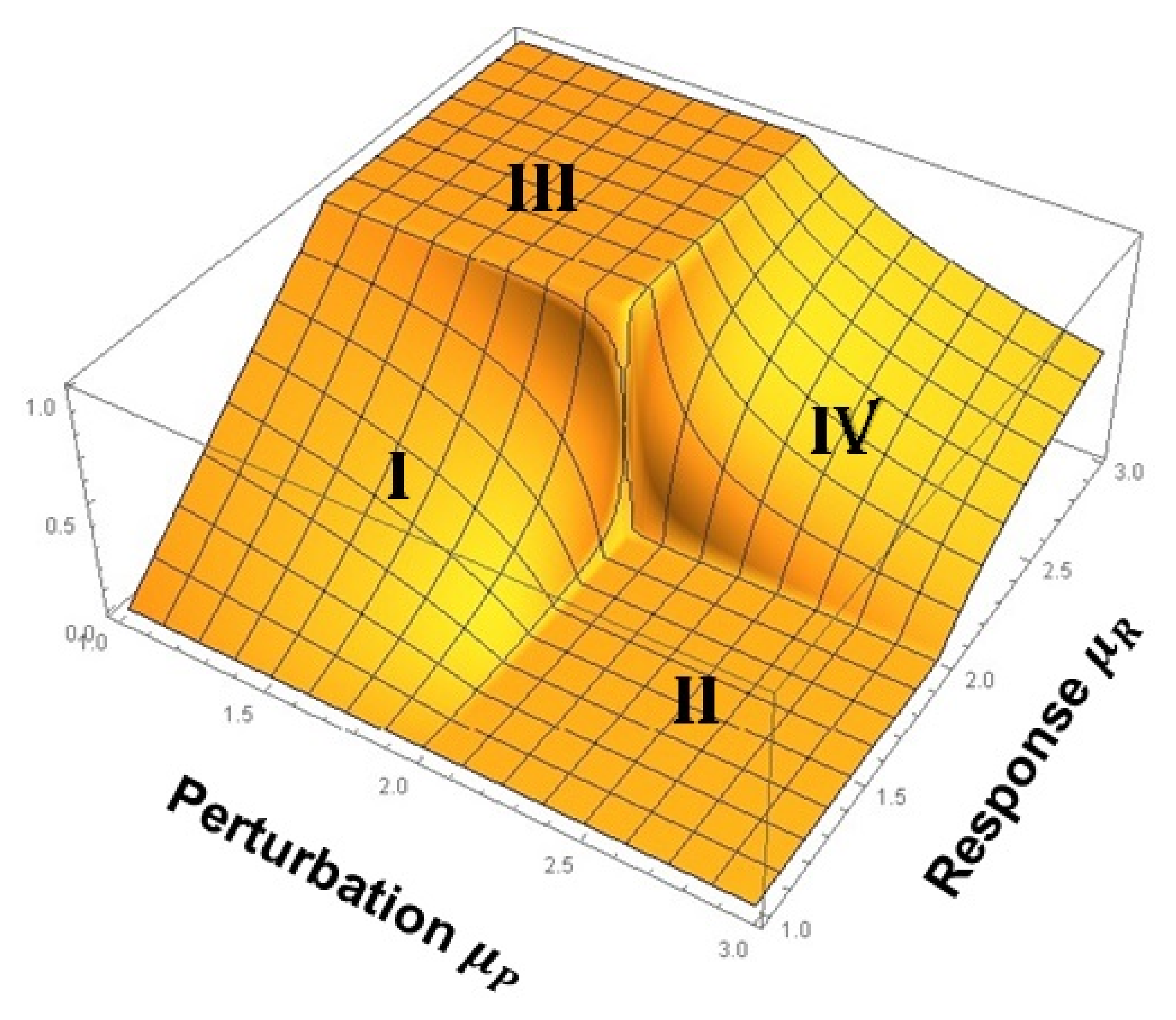
In Figure 6, the asymptotic cross-correlation function, evaluated using ensemble distribution functions, is normalized to one and graphed as a function of the IPL indices of the two networks to form a cross-correlation cube (CCC). As mentioned, captures the complexity of the perturbing network and that of the responding network; and taken together, these values define a plane. The value of the cross-correlation function at each point on the plane defines a third dimension, so that the three together give rise to the CCC. Note that this cube denotes the asymptotic values of the cross-correlation function and displays a number of remarkable properties.
In keeping with our definition of complexity, the networks of interest are complex and each have an IPL strictly in the domain and we do not truncate the time series in the calculations as we did in the multifractal time series perturbation calculations. For the moment, we focus our attention on networks whose complexity is high corresponding to (region 1) and networks whose complexity is lower corresponding to (region 2). Summarizing the asymptotic influence of one network in a given complexity region on another network in a second complexity region, it has been shown that [2,40,41]:
- (1)
- A complex network belonging to region 2 cannot exert any asymptotic influence on a complex network belonging to region 1. This is the square denoted II on the CCC and is where LRT supposedly died.
- (2)
- A complex network belonging to region 2 exerts varying degrees of influence on a complex network belonging to region 2. This follows from PCM and is indicated by IV on the CCC.
- (3)
- A complex network belonging to region 1 exerts varying degrees of influence on a complex network belonging to region 1. This follows from PCM and is indicated by I on the CCC.
- (4)
- (5)
- When the two IPL indices are equal to 2 there is an abrupt jump up from zero (square II) to one (square III), or down from one to zero, depending on the values of the IPL indices just before they converge on 2. This is a singular point where the spectra of the two networks display exact -noise fluctuations.
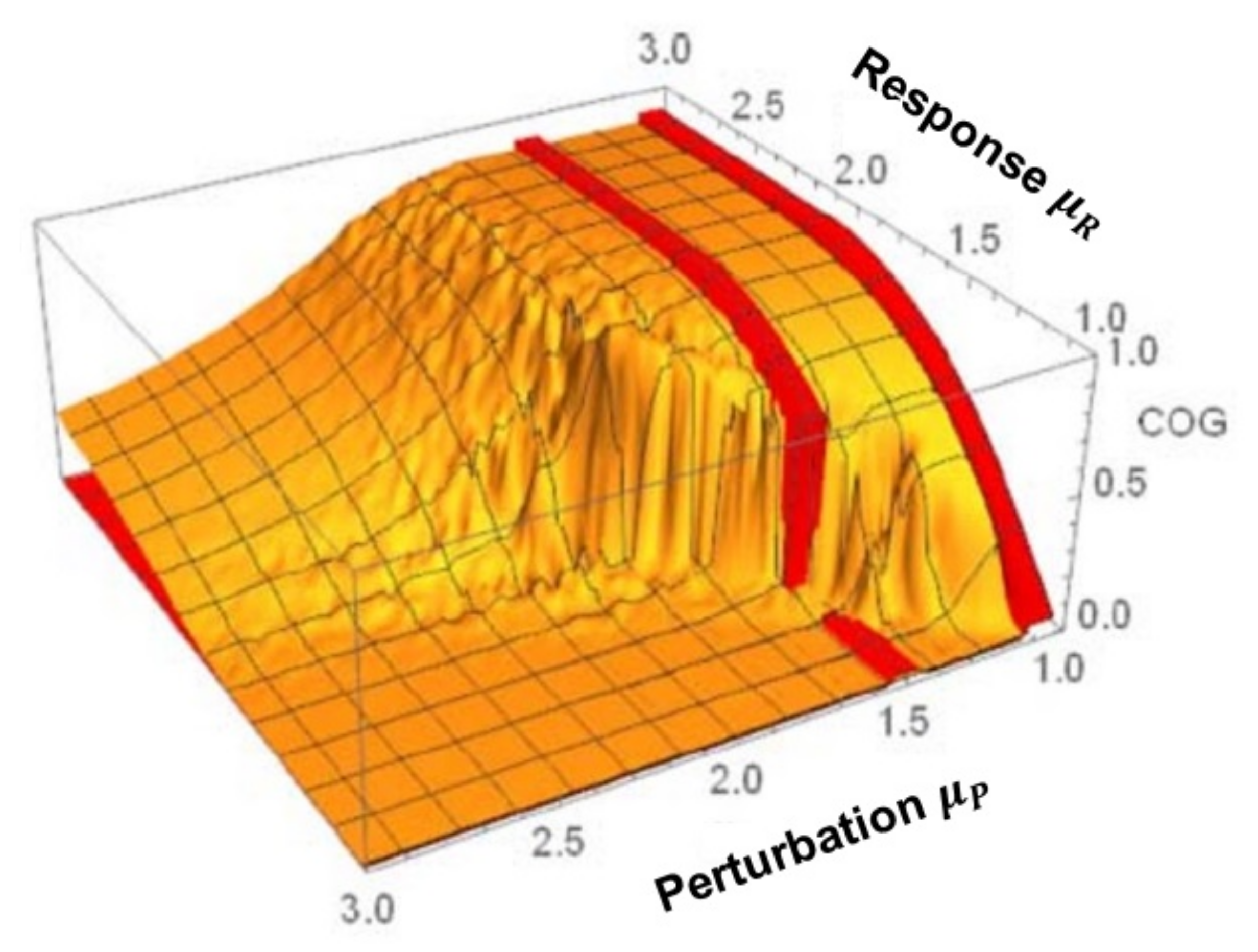
It is possible that one could have extrapolated the results obtained for the transfer of multifractal behavior between complex networks discussed in the preceding section to sketch the results obtained from the CCC—at least in the case where the regions in which the two networks were generating ergodic time series, i.e., where the IPL indices were both in region 1. Things are more complicated when one network is ergodic (region 1) and the other network is non-ergodic (region 2). Piccinini et al. [41] were able to prove that a nearly identical CCC to that depicted in Figure 6 could be numerically constructed using time averages rather than ensemble averages by being cautious with the numerics. The latter CCC is referred to as the Non-Ergodic Complexity Management CCC and is include here as Figure 7 for ease of reference.
The main result of this section is a demonstration that the mechanism that gives rise to the exchange of information between two complex networks, following as it does from the PCM [37,39], is the same as that which transfers multifractal properties from one network to the other, that mechanism being the information gradient arising from the relative complexity and thereby producing an information force [76]. It is also worth emphasizing that all the results obtained here for the interaction of two complex networks were also obtained using yet another method in a recent paper [103].
4. Fractional Calculus
The Introduction briefly presented the case for not being able to use the IC to successfully demystify complex phenomena and thereby not be able to replicate in the life sciences the success enjoyed in the physical sciences by the use of IC dynamic models. At its core, the barrier to be overcome is the inability to define complexity using a reductionistic approach. One of the clearest discussions of the distinction between complicated and complex networks is given by Deligniéres and Marmelat [57], wherein a complex phenomenon is argued to consist of a very large number of infinitely entangled components such that the phenomenon cannot be decomposed into elementary units. In such a network, the interactions are more important than the components themselves, and the whole is greater than the sum of its parts.
Just as Newton’s shift from the positional focus of geometry to that of motion was entailed by his fluxions, along with the eventual development of the reductionist perspective of science, so too is a modern-day shift from simplicity to complexity entailed by the giant steps made in our ability to measure, coallate and compute. Consequently, today’s situation is thought to be comparable to the time of Newton requiring a new way of thinking, in large part because of the confusion over how the world’s complexity influences our undertanding of the world.
There is the mathematics that all the physics community knows and understands, which is dominated by the IC paired with Newton’s forces. However, this robust view of how to understand the world has been subverted by the three-body problem, where, as described by Poincaré, a planet orbiting two suns finds itself on a fractal trajectory (of course, the term fractal did not come into existence for another 100 years in the work of Mandelbrot). More generally, a non-linear mechanical system with three or more degrees of freedom is chaotic [121] and, given the proper conditions, a trajectory can break up into a spray of points [122], or, if dissipative, can be drawn onto a fractal attractor [123]. This state of affairs was summarized by Sir James Lighthill, a leader in applied mathematics, who in 1986, when he was the president of the International Union of Theoretical and Applied Mechanics, presented a paper to the Royal Society entitled The recently recognized failure of predictability in Newtonian dynamics [124]: (It is probably worth pointing out here that a reviewer suggested deleting this quote from from this paper. My reluctance to do this stems from the fact that the strength of science is, in part, a consequence of the willingness to acknowledge mistakes made being a necessary part of the process. The more fundmental the error, say one of interpretation, the more value associated with its uncovering. Few scientists today remember the luminiferous aether or spontaneous generation, but might recall phlogiston theory or even more recently cold fusion. These conceptual errors stood as barriers to understanding the true nature of the phenomenon being misunderstood and their removal was necessary in order to move forward using the knowledge gained from those mistakes).
We are all deeply conscious today that the enthusiasm of our fore bears for the marvelous achievements of Newtonian mechanics lead them to make generalizations in this area of predictability which, indeed, we may have generally tended to believe before 1960, but which we now recognize were false. We collectively wish to apologize for having misled the general educated public by spreading ideas about determinism of systems satisfying Newton’s laws of motion that, after 1960, were to be proved incorrect…
In this section, we consider how the FC can bridge the gap between the multifractality of empirical time series and the equations of motion required to described the behavior of the phenomena generating the multifractal time series. The familiar phenomena of motor mobility by walking, exchanging CO for oxygen to fuel the body through breathing, and circulating the blood to supply oxygen and nutrients to the body by the heart pumping blood, share a common feature having to do with the variability in the frequency of their cycles. Heart rate variability (HRV), breath rate variability (BRV), and stride rate variability (SRV) each provides a distinct measure of the statistical changes in a nearly cyclic underling process. Many of the physiologic details leading to the inescapable conclusion that each of these processes is multifractal in nature have been recorded [37]. In fact, multifractal time series appear to be ubiquitous in biomedical phenomena.
In prequel II, we reviewed the evidence for the need to describe the dynamics of fractal phenomena by the FC with constant fractional-order (FO) derivatives. Herein, we use the FC with FO derivatives that are stochastic to establish the required equations of motion for multifractal phenomena. We use datasets of rate variability of physiologic processes to securely establish the need for such FC equations of motion to describe the dynamics of complex physiologic phenomena.
4.1. Nexus with Multifractality
The nexus of multifractality and the FC can be established using a number of modeling strategies. A rather broad review of the fractal time series that arise in physiology and medicine was presented in prequel I. The mathematical properties of these empirical fractal time series were used to establish that the IC was not sufficient to model these phenomena, because the evolution of fractal functions over time do not have traditional integer-order equations of motion. A brief introduction to the FC was provided therein in anticipation of the more extended discussion of the formalism in prequel II.
The utility of the FC in determining the properties of physiological networks was taken up in prequel II, including a summary of how to solve certain fractional equations of motion, and which will not be reproduced here. However, we did replace integer-order (IO) growth models, both linear and non-linear, with FC generalizations and discussed the network properties entailed for each kind of generalization. Two distinct arguments were made in making these replacements; one based on the network effect and the other on the time subordination method. These were followed by a third generalization in making the fractional-order index of the time derivative itself a function of time .
The primary focus of the time dependence of the non-integer index discussed in prequel II was to demonstrate the utility of a time-varying order parameter using a previously fitted tumor growth dataset. This was achieved using an exploratory approach and captured the 14 data point history of a tumor by the time-dependent value of the order of the time derivative using Taylor series [125]. We do not reproduce those results here but instead take the next logical step and consider two additional kinds of variability in the derivative parameter by considering the effect of the order of the derivative being either a random or a stochastic variable.
The latter equations address fractional Langevin equations (FLE) and introduce the need for a fractional probability calculus (FPC).
4.1.1. Fractional Linear Langevin Equation (FLLE)
The proposed fractional linear Langevin equation (FLLE) can be cast in the form:
where is a zero-centered random force, is the Riemann–Liouville fractional derivative of order , the range of the fractional index is , the constant has the dimensions of 1/time, and is the dynamical variable of interest. Finally, the quantity is the Euler integral of the second kind and is called the gamma function [126]. Note that the dynamic variable does not need to be continuous at the origin, nor does it need to be differentiable. The solution to this equation is obtaind in prequel II:
where for ease of notation we choose . Averaging this solution over the fluctuations in the additive random force, indicated by a suitably subscripted bracket, yields:
The solution to the fractional-order equation with no random force was first obtained by the mathematician Mittag-Leffler at the turn of the 20th century in terms of the series which now bears his name:
the Mittag-Leffler function (MLF).
This FLLE was used to model the influence of a network on the probability that a single element in the network will change its decision (state) [60]. As mentioned, this was termed the network effect and describes how a network consisting of N interacting element influences the behavior of a single element. In the decision-making model (DMM), the network is described by integer-order dynamic equations for the probability of each of the network members being in one of two states. These equations were transformed into one fractional-order (FO) equation of motion for a typical individual in the network. The solution given by Equation (16) is shown in Figure 2 of prequel II to coincide with the numerical calculation of the survival probability of a single element in a 10,000 element network. Here, the MLF is the homogenous solution and is also the Greens function weighing the contribution of each fluctuation to the nuanced changes in opinion of an individual element due to the influence of the other 9999 members of the network.
In this case, the non-integer order of the fractional derivative is obtained as a fitting parameter to the results obtained by large-scale numerical calculations. However, we do not have, as yet, a theory explicitly relating to the detailed properties of the numerical calculation, which is to say, we do not see the connection between the properties of the network and the fractional rate equation for the individual member of the network. However, we do see that the FC equation is a consequence of the critical dynamics of the network and is like the mathematical theorem of Carlman that tells us that a finite dimensional non-linear dynamical system has an equivalent infinite dimensional linear system description, but does not indicate how to construct the latter representation of the former. The network effect we discovered is like that and remains an intriguing formal result supported by numerical experiment [60].
4.1.2. Stochastic Fractional Index
An even simpler FLE can provide us with insight into the influence of another kind of FO. Consider the dissipation-free form of the FLLE, i.e., , whose formal solution is:
where is the kernel corresponding to the dynamic operator in Equation (14):
which can be interpreted as a filter and . The simplest FLE (SFLE) to which Equation (18) is the formal solution could be obtained from the construction of the FLE for a free particle coupled to a fractal heat bath when the inertial term is negligible [127].
As written, the solution to the SFLE is a monofractal if the statistics of the random force are specified to be monofractal. What makes the solution a multifractal time series is choosing the index of the fractional operator to also be a random variable. Generally, if the additive random force is chosen to have fractal Gaussian statistics, it scales as:
which, for a Wiener process, has [44,51]. The kernel given by Equation (19) scales as:
consequently, the solution to the SFLE scales as:
The time dependence of the second moment is given by which is obtained by inserting into Equation (22) and it agrees with the second moment obtained for anomalous diffusion if we identify with the Hurst exponent. If the stochastic force is that of classical diffusion, that is, and , then the interval of values for the fractional operator index in Equation (18) is given by . Consequently, the process described by the SFLE can cover the full range of values .
Multifractals: As reviewed in [65], the interval has in the past been interpreted in terms of an anti-persistent random walk. An anti-persistent explanation of time series was made by Peng et al. [10] for the differences in time intervals between heart beats, now called HRV. They interpreted their time series, as did a number of subsequent investigators, in terms of random walks with . In this model, the anti-persistent behavior lead to an avoidance of the extremes, so that the time intervals became neither too large nor too small. However, from these results, it is clear that the SFLE as a model for the dynamics provides an equivalent description of the underlying dynamics. The scaling behavior alone cannot distinguish between these two models. What is needed is a complete statistical distribution and not just the time dependence (scaling behavior) of the central moments.
There are a number of ways to test the interpretation of the scaling behavior observed in Equation (18). For example, Podlubny [128] showed that when reality manifests the dynamics of a FO, rather than an IO, differential equation, attempting to control it with IO feedback leads to extremely slow convergence, if not divergence, of the network output. On the other hand, using a FO feedback, with the indices appropriately chosen, leads to rapid convergence of the output to the desired signal. Thus, we anticipate that dynamic physiologic networks with scaling properties, because they can be described by fractional dynamics, would have FO controls.
The solution to the SFLE is monofractal if the additive fluctuations are monofractal. One way to make the solution to the SFLE a multifractal when the fluctuations of the random force are monofractal is to assume that the parameter in the kernel given by Equation (21) is a random variable. To construct the traditional measures of multifractal statistical processes, we calculate the qth moment of the solution Equation (22) by averaging over both the random force and the random parameter to obtain [78]:
Consequently, when the exponent in the memory kernel in the SFLE is random, the solution consists of the product of two random quantities, giving rise to a multifractal process. To determine the structure function exponent , we make an assumption about the statistics of since we can always write the average as:
where is the random variable. The expression on the RHS of this equality is the Laplace transform of the PDF.
We assume the random variable has Lévy statistics so that the PDF is given by:
with and . Inserting the PDF into the average and integrating over z yield the delta function , which integrating over k in the Fourier transform yields:
so that the structure function exponent extracted from Equation (23) can be written:
This expression produces a q-order structure function exponent determined by the scaling relation in Equation (23). Note that if the structure function exponent is linear in q, the underlying process is monofractal, whereas, when it is non-linear in q, the process is multifractal. The structure function exponent has been related to the mass exponent [129]:
Consequently, we have so that , as it should because of the well-known relation between the fractal dimension and the global Hurst exponent .
Note that for an infinitely long time series, the Hölder exponent h and the Hurst exponent H are identical; however, for a time series of finite length, H and h are not necessarily the same. We stress that the fractal dimension and the Hölder exponent are local quantities, whereas the Hurst exponent is a global quantity, consequently the relation is only true for an infinitely long time series. The multifractal spectrum describes how the local Hölder (fractal) exponents contribute to such time series.
We can see from Equation (24) that the solution to the SFLE corresponds to a monofractal process only in the case that and , otherwise the process is multifractal [50].
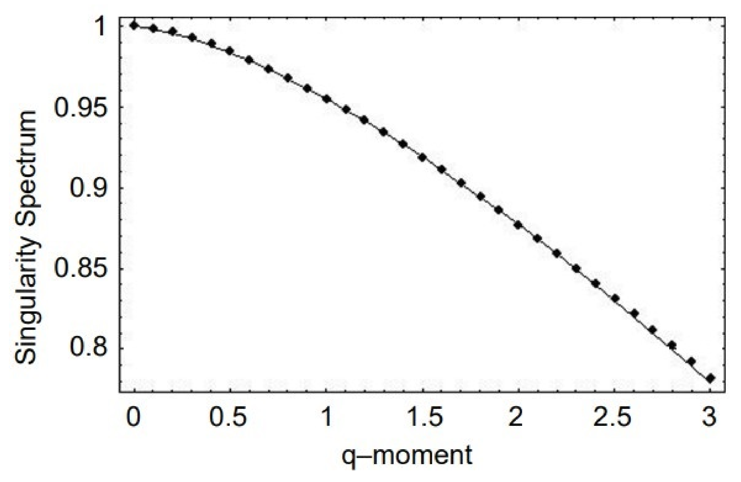
This approach has been applied to BRV, HRV, and SRV time series datasets and interpreted for the statistics of the FO exponent given by Lévy statistics. The singularity spectrum as a function of the positive moments shown by the points in Figure 8 for human gait data. The solid curve in this figure is obtained from the analytic form of the multifractality spectrum:
which was determined by substituting Equation (24) into the equation for the singularity spectrum given by Equation (12), through the relationship between exponents Equation (25). It is clear from Figure 8 that the data are well fit by the solution to the SFLE with the parameter values and , obtained through a mean square fit of Equation (26) to the SRV time series datasets.
As mentioned earlier, the multifractal spectrum for the middle CBF velocity time series for a healthy control group using the solution to a linear Langevin equation [130], was compared with a group of migraneurs as depicted therein in Figure 11. We note here that in the fit to the spectrum using Equation (26), indicating that the statistics of the fractional-order derivative in this case is Gaussian, that being the only member of the Lévy PDFs that has a finite variance. An alternative way to express the singularity spectrum the CBE is:
where we observe that the fractal dimension is given by , which is the value of the spectral function at . The width of the multifractal distribution for the CBF velocity of the migraneurs is constricted by a factor of three from 0.038 averaged over the control group to 0.013 averaged over the group of migraineurs, suggesting that the underlying process has lost a great deal of flexibility. However, both of these multifractal spectra are centered at so that the average scaling behavior between the two groups remains the same.
It is the case that disease—here, that is migraine—may be associated with the loss of complexity [131]. Complexity is lost along with flexibility in proportion to the narrowing of the spectral width, and consequently the loss of adaptability, thereby suppressing the normal healthy multifractality of blood flow within the brain. More generally, the narrowing of the multifractal spectrum indicates a loss of adaptability of the associated physiologic network and therefore there is an attendant reduction in the network’s ability to carry out its function. This may also suggest the reason for the associated headache, since pain is often the biomedical indicator of a network’s inability to preform its function.
5. Fractional Probability Calculus
It is useful here to recall the two paths that lead many if not most physical scientists to an understanding of uncertainty in the dynamics of physical processes, which is nowhere better contrasted than in the distinct treatments of Brownian motion by Einstein [132] and Langevin [133]. Each investigator explained the uncertain influence of the environment on the movement of the Brownian particle in their own way; Einstein used the physical notion of probability in phase space in a thermodynamic analysis, whereas Langevin used the idea of random forces resulting from the dynamic equations. However, both were satisfied that the Brownian particle moved according to Newton’s force law, but they differed in the manner of taking into account the thermal motion of the environment on the Brownian particle’s motion.
In prequel II, the IO force laws were replaced with FO force laws based on empirical evidence. For example, this replacement was proposed when an ostensibly deterministic linear process of interest yielded experimental results that systematically deviated from any linear Newtonian model of the phenomenon. When such a process was described by a fractal rate equation (FRE) as, for example, given by the generalization of Newton’s law of cooling by Mondol et al. [134], the Newtonian IO model was abandoned in favor of the FO model.
When the process of interest is a monofractal, its IO derivative diverges, but a FO derivative of that same function is well defined, with only a shift in the fractal dimension resulting [135]. Consequently, we argued that the equation of motion for a process described by a fractal function must contain FO derivatives and the solution to such equations are formally expressed in terms of FO integrals.
5.1. Fractal Diffusion
The traditional discussion of the LE typically begins with Newton’s force law for a system of interest coupled to the environment. The description developed in any of a number of excellent texts on statistical mechanics [136,137] expresses the coupling of a system to its environment through a deterministic force and a random force. The first and second moments of the dynamic variables in the LE are then used to construct the Fokker–Planck equation (FPE) for the corresponding PDF. The simplest FPE is that for a freely diffusing particle:
where the dependence of the PDF on the initial state is not explicitly indicated, x is the dynamic variable and the diffusion coefficient D is related to the mean-square strength of the random force. The corresponding LE given by:
and is a memoryless Wiener process. The Gaussian PDF is obtained by solving the FPE for a delta function in space initial condition, or by inserting the time integral over the fluctuations in the LE into the characteristic function and using the properties of the Wiener process to obtain the PDF. All of this has been known since the turn of the last century. Knowledge of a more recent vintage has to do with replacing the LE Equation (28) with the FLLE and the solution to which is given by Equation (18).
Consider a random walk (RW) process to model the LE given by Equation (28). The properties of the RW determine the statistics of the random force along with its correlation properties. We select to be a dichtomous unit step process such that whose two-point autocorrelation function has the stationary form:
The probability that the dynamic variable has the value in the phase space interval () at time t is , and its evolution is determined by the diffusion equation [130,138]:
Note that here the diffusion equation is a convolution in time and that the autocorrelation function plays the role of a memory kernel.
Lévy statistics: The theory of the influence of long-time memory on stochastic phenomena was developed to explain diffusion in which the second moment of the diffusion variable does not increase linearly in time, that is, the diffusion is anomalous. Following West et al. [130], this long-time memory is captured by assuming an IPL form for the autocorrelation function:
with and from the second moment yields for the Hurst exponent , from which the discussions for Brownian motion follow.
Under the assumption that the RW is constrained to walkers whose steps have a constant finite speed, say unity, such that the two positions x and are related through the two times t and
where the Dirac delta function confines the step size due to the finite speed of a step. Allegrini et al. [138] show that this expression enables the rewriting of Equation (30) without approximation as:
where b and are each a collection of known constants and we have used . Making the plausible assumption that the short-range region does not contribute to the long-time evolution of the PDF, Equation (33) becomes identical to the fractional diffusion equation for the PDF:
where and the operator is the Riesz–Feller fractional derivative [139].
The characteristic function is given by the Fourier transform of the PDF:
such that [7]:
and the Fourier transform of Equation (34) becomes a rate equation for the characteristic function:
The inverse Fourier transform of the solution to the rate equation with the initial condition therefore yields the Lévy stable PDF:
and does not have a simple analytic form except for a few values of the Lévy index among which are the Gaussian for and the Cauchy for . Note that the Lévy PDF satisfies the scaling relation given by Equation (6), where the scaling index is and the function is a known integral in this case.
Fractional in time and space: Memory can be introduced into the FPE by means of a subordination process whereby two times are introduced into the process and one is subordinated to the other. The concept of using different clocks to measure different aspects of interacting complex dynamic networks dates back to the middle of the 19th century. It was then proposed that the two clocks defined subjective and objective times and were used to justify the empirical Weber–Fechner law [140]. Due to the present-day availability of time resolved datasets, life science investigators have begun adopting the notion of multiple clocks to distinguish between cell-specific and organ-specific clocks in biology, which is analogous to person-specific and group-specific clocks in sociology. While the global activity of an organ, such as the brain or the heart, might be characterized by quite regular behaviors, the activity of single neurons or pacemaker cells demonstrate statistical intermittency resulting in global 1/f variability.
In this way, interpreting the time in Equation (27) as the intrinsic time of the system of interest and subordinating that time to the clock time of the environment yields [7]:
which was called fractional time FPE. The fractional time derivative is of the Caputo type, which, for the purposes here, we define in terms of its Laplace transform:
where the Laplace transform of is and the initial state of the PDF is given by the Dirac delta function: .
Of course introducing subordination into the simplest FPE was an arbitrary choice. It is probably more reasonable to consider subordination in a network where spatial heterogeneity is also present and for that you need a fractional kinetic theory (FKT). Zaslavsky [141] considered chaotic dynamics to be the bridge between deterministic and stochastic dynamic systems, and developed the mathematics for the fractional kinetics corresponding to chaotic dynamics intermediate between completely regular (integrable) and completely random networks. The kinetics are “strange” in that the low-order moments of the PDF can be infinite and the Onsager Principle is violated because it takes infinitely long for fluctuations to relax back to the equilibrium state. West and Grigolini [130] present an alternative to the fractional kinetic equation (FKE) developed by Zaslavsky [141].
Zaslavsky’s arguments [141] lead to a FKT resulting from the underlying dynamics being chaotic and consequently to the dynamic trajectories being fractal. The historical kinetic theory argument was generalized by taking into account the fractal nature of the set generated by the ensemble of chaotic trajectories initiated by a non-integrable Hamiltonian. Inserting the time limit for a fractional time differential into the chain condition for a stationary PDF yields:
where is the stationary PDF of having a particle at position x a time after it was at the position y. This expression can be simplified by introducing the generalized Taylor expansion:
for a set characterized by the fractal dimension . (Note that this is only a sketch of the much more detailed arguments presented by Zaslavsky. The purpose here is to show the connection between the FC and multifractality). Inserting this expansion into Equation (40) simplifies the generalized chain condition by introducing the quantity:
to obtain the fractional Fokker–Planck equation (FFPE):
The FFPE has fractional indices in the domains and , the fractional time derivative is of the Caputo form, and the fractional spatial derivative is of the symmetric Riesz–Feller form.
Zaslavsky [142] explained that the limit in Equation (42) is the result of the fractal dimensionality of the space–time set, along which the state of the system is meandering in the limit. In this all too brief discussion of Zaslavsky’s contribution to a FKT, we should mention the work that he along with collaborators did to visualize the underlying landscape produced by averaging over chaotic trajectories, which enabled them to describe the formal structure uncovered by extensive numerical calculations. They discuss the idea of a “stochastic web” characterizing the dynamics in which “weak” chaotic orbits, generated by Hamiltionian systems, are concentrated on small measure domains of phase space thereby constituting a “web”. This argument can be recast as a random walk which we do in the next section.
They note that transport through stochastic webs could produce non-Gaussian, i.e., intrinsically anomalous, diffusion. We do not reproduce the mathematical details from the open literature and instead jump to the result for the one-dimensional fractional kinetic equation (FKE) [130,142] for one of the simplest dynamical processes described by the FFPE, thereby reducing Equation (43) to:
This is one of the simplest forms of anomalous diffusion, first discussed in terms of the continuous time random walk (CTRW) by Montroll and Scher [143].
The solution to this fractional diffusion equation is readily obtained by taking its combined Fourier–Laplace transform to obtain from the Fourier–Laplace transform of the FFPE:
where the astrix denotes the double transform of the PDF. This equation is simplified for the initial value problem ⇒ to the form:
The inverse Fourier–Laplace transform of this expression yields the solution to the initial value problem for the PDF.
Metzler and Klafter [144] derived the FFPE using the CTRW formalism of Montroll and Weiss [145] and reviewed the potential functions for various combinations of indices. It was also derived using subordination theory by West [139]. The inverse Laplace transform of yields the characteristic function:
expressed in terms of the MLF given by Equation (17). The inverse Fourier transform of the characteristic function yields the PDF solution:
The simple substitution into Equation (48), with after some algebra reduces the formal solution to:
or in a more familiar scaling form given by Equation (6), where the new function is defined from the inverse Fourier transform in Equation (49). The new function is analytic in the scaled variable , is properly normalized and can therefore be treated as a PDF. For a diffusion process with no intrinsic memory, ; in which case, the MLF becomes an exponential so that for , the Fourier transform can be carried out and this function becomes a Gaussian with . When and , the result is a stable Lévy process [146,147] with the Lévy index given by . However, for general chaotic systems, there is a broad class of distributions for which the functional form is neither Gaussian nor Lévy.
Mainardi et al. [148] obtained a variety of other solutions to the FKE in terms of the properties of the MLF for . The inverse Fourier transform of the scaled PDF solution for asymptotically relaxes as the IPL in time with an IPL index .
5.2. Fractal Random Walks
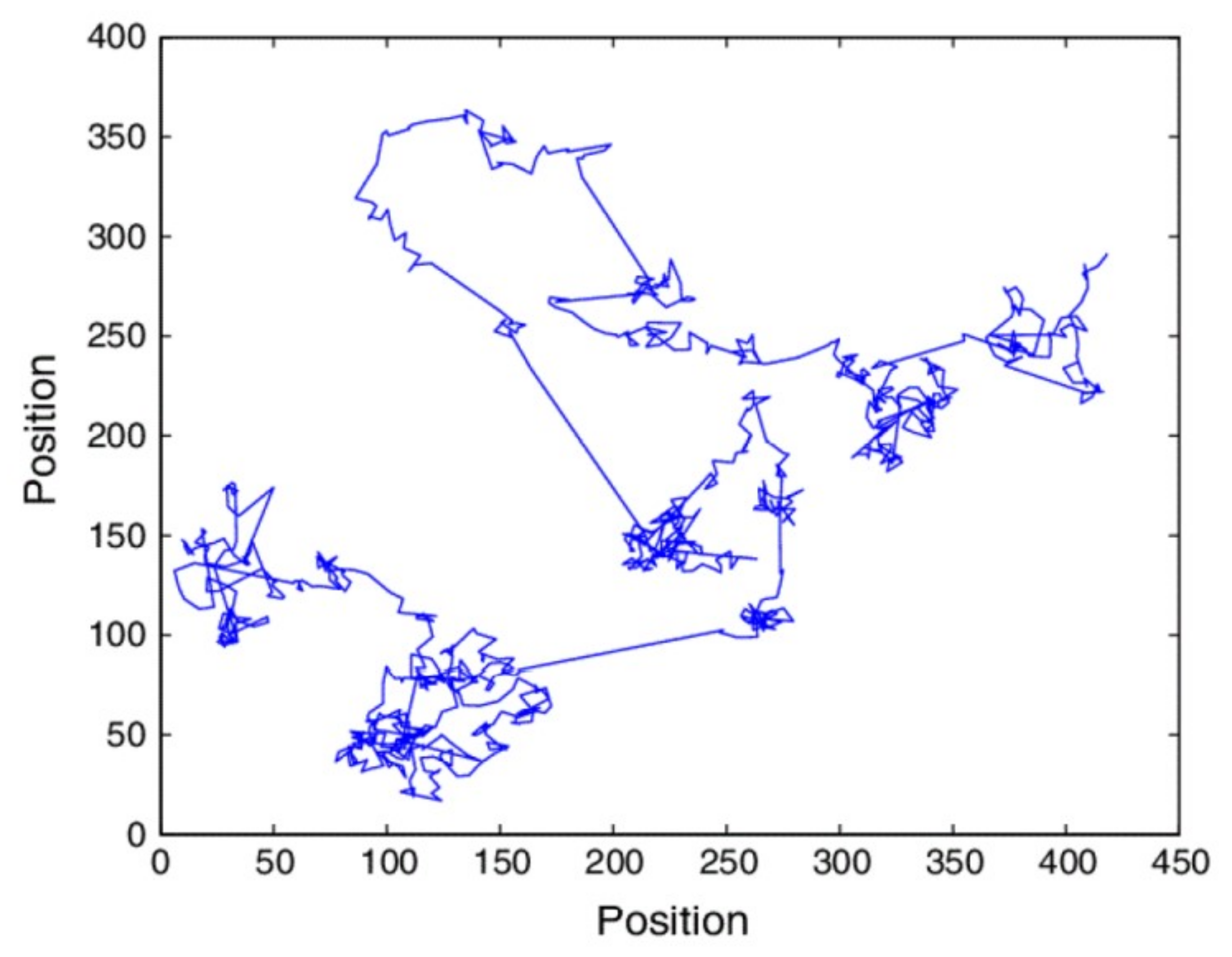
The web connectivity discussed by Zaslavsky is made up of traps where homoclinic points have dissolved into sprays of local points that locally entrap trajectories for sojourn times of intermittent length described by an IPL of waiting times. Once it has exited a trap, the trajectory undergoes a long-range flight having self-similar properties. This argument can be realized by replacing the complete simulation of the Hamltoian dynamics involving turnstiles and cantori [149] with a RW containing the approriate features. This can be performed using a RW determined by a Weierstrass (W) function to construct a Weierstrass random walk (WRW) for a discrete PDF with sites on a one-dimensional lattice indexed by x [150]:
As the WRW process unfolds, the set of sites visited mimics the influence of localized chaotic islands, interspersed by gaps, nested within clusters of clusters over ever-increasing spatial scales. The WRW generates a hierarchy of traps that are statistically self-similar, as suggested by the RW process depicted in Figure 9. The parameter a determines the number of subclusters within a cluster and the parameter b determines the scale size between clusters subject to the condition , which ensures that the second moment diverges.
The discrete Fourier transform of Equation (50) yields the characteristic function which has the form of a Weierstrss function (WF). The solution to the WRW can be determined analytically using the scaling properties of the WF to apply renormalzation group theory. The complete characteristic function has a homogeous and a singular part; the former is analytic in the neighborhood of and the latter is singular in this neighborhood. We obtain the scaling relation for the singular part of the characteristic function:
which has the renormalization group solution:
with the complex power law index:
The analytic forms of the Fourier coefficients in Equation (52) are given in [150].
They [150] establish that the dominant behavior of the WRW is determined by the lowest-order term in Equation (52), and the term in the series: whose inverse Fourier transform is determined by a Tauberian theorem to be the IPL:
and is a known function of . Thus, the singular part of the WRW has an IPL stepping PDF and this dominant behavior intuitively justifies ignoring all the other terms in the series.
We can now write for the asymptotic time-dependent form of the discrete PDF resulting from the WRW process:
in which each step n in WRW process occurs at equal time intervals. This equation was analyzed by Gillis and Weiss [151], who determined that its solution to a Lévy PDF, thereby relating the RG solution of the WRW to the discussion of the FDE.
Stable Lévy processes can therefore arise from the “weak” chaotic nature of the phase space trajectories. This is, in part, a consequence of the asymptotic behavior corresponding to the asymptotic , which is of significance in determining the transport behavior of the anomalous diffusion process.
6. Discussion and Conclusions
One difficulty encountered in writing a sequence of interrelated essays is the challenge of restricting the discussion and conclusions to the narrow perspective of a single essay. In prequel II, it was found that rather than attempting a detailed summary of what had been presented therein, the general results obtained were instead itemized and their significance articulated. This strategy turned out to be successful and we apply it here as well.
Let us begin by identifying the most important points covered in the two prequels and touched on herein as well:
- (1).
- The simple analytic functions of the IC have been found to be insufficient to describe the time dependence of most physiology networks. The notion of fractality was introduced to capture the true complexity of such biomedical network time series through fractal geometry, fractal statistics and fractal dynamics.
- (2).
- A fractal function diverges when an integer-order derivative is taken, so that such a fractal function cannot be the solution to a Newtonian equation of motion. However, when a fractional-order derivative of a fractal function is taken, it results in a new fractal function. Consequently, a time-dependent fractal process can have an equation of motion that is a FDE.
- (3).
- The network effect is the influence exerted by a complex dynamic network on each member of the network. When the network dynamics is a member of the Ising universality class, the interconnected set of IDEs for the probability of an individual being in one of two states during its non-linear interaction with the other members of the network can be replaced by an equivalent linear FDE and solved using the FC.
- (4).
- Even the simplest FDEs has a built-in memory resulting from the hidden interaction of the observable with its environment, which is manifest in the non-integer order of the time derivative, as in the network effect.
- (5).
- The solution to a linear FRE is a MLF for and becomes an exponential function for . The MLF is the workhorse of the FC just as the exponential is for the IC.
- (6).
- A truly complex stochastic dynamic process can have more than one fractal dimension. A multifractal process is characterized by a uni-modal spectrum peaked at the value of the Hurst exponent .
These points have been developed further in the present essay whose most important points are as follows:
- (7).
- The flow of information due to interaction of two complex networks each generating a multifractal time series is from the network with the broader to that with the narrower multifractal spectrum. This is summarized in the interpretation of the efficiency of information transfer using the CCC.
- (8).
- FREs with random fractional derivatives are shown to generate multifractal processes and therefore can be used to model the dynamics of both healthy and pathological physiologic networks.
- (9).
- Multifractality emerges from three distinct sources: (1) the introduction of random fractional derivatives into the dynamics of complex networks; (2) a FKT developed to define the evolution of PDF over fractional trajectories; (3) fractional random walks with diverging central moments.
- (10).
- A simple FDE that has a built-in non-locality in space is the FSDE. The solution to this fractional diffusion equation in space is a Lévy PDF, whose index is given by the order of the spatial fractional derivative. Yet another fractional diffusion equation differs in having a built-in memory and is the FTDE. The solution to this fractional diffusion equation in time is expressed in terms of the inverse Fourier transform of a MLF.
- (11).
- The health of a physiologic network is manifest by the width of the multifractal spectrum of the time series generated by that network. Experiments include but are not limited to CBF, HRV, BRV and SRV, which also show that pathologies in each of the underlying networks narrow the approprate multifractal spectrum.
The empirical evidence supports the interpretion that physiologiv time series are described by fractal stochastic networks. Moreover, the fractal nature of these time series is not constant but often changes with the vagaries of the interactions of one network with another, since other networks are the environment in a network of networks. In addition, there is the SOTC produced by a network’s internal dynamics. Consequently, physiologic phenomena are nearly always multifractal and the multifractal spectral width is a measure of the state of health of that network.
A remarkable aspect of multifractality is that it is not just a consequence of the critical dynamics of complex networks, inwhich SOTC would be a reasonable driver for such behavior. The three-body problem and its subsequent generalization to chaos theory along with the limited predictability of non-linear dynamics systems hold the key to deciphering the information contained in physiologic time series. Nature uses multifractality to adapt to the breakdown of classical dynamics into chaos, resulting in fractal trajectories to go a step beyond what Taleb called ’antifragile’ behavior [152]. The antifragility concept articulates how things gain from disorder rather than being weakened by it. The enhanced uncertainty that antifragility promotes in order to become stronger in the face of disruption and adversity, whether internally or externally produced, is precisely what is measured by the width of the multifractal spectrum.
The degree of flexibility required to attain and maintain health is part of the stochastic control process that for generations was interpreted as random noise in physiologic time series. It seems to the author that rather than being noise, the multifractality character of physiologic time series is nature’s real-time prescription for how to adapt and survive.
Funding
The author received no external funding to support this research.
Institutional Review Board Statement
Not applicable.
Informed Consent Statement
Not applicable.
Data Availability Statement
Not applicable.
Acknowledgments
The author acknowledges the many investigators whose work are freely drew from and cited herein.
Conflicts of Interest
The author declares no conflict of interest.
Nomenclature
The following abbreviations are used in this manuscript:
| BRV | breathrate variability |
| GLRT | generalized linar response theory |
| CBF | cerebral blood flow |
| HRV | heartrate variability |
| CCC | cross correlation cube |
| IC | integer calculus |
| CE | crucial event |
| IDE | integer differential equation |
| CTRW | continuous time random walk |
| IPL | inverse power law |
| DMM | decision-making model |
| LE | Langevin equation |
| FBM | fractional Brownian motion |
| LRT | linear response theory |
| FC | fractional calculus |
| MLF | Mittag-Leffler function |
| FDE | fractional diffusion equaton |
| PCM | principle of compexity management |
| FFPE | fractional Fokker–Planck equation |
| probability density function | |
| FKE | fractional kinetic equaition |
| RG | renormalization group |
| FKT | fractional kinetic theory |
| RHS | right hand side |
| FLE | fractional Langevin equation |
| RW | random walk |
| FLLE | fractional linear Langevin equation |
| SFLE | simplest fractional Langevin equation |
| FO | fractional order |
| SOC | self-organized criticality |
| FPE | Fokker–Planck equation |
| SOTC | self-organized temporal criticality |
| FPC | fractional probability calculus |
| SRV | striderate variability |
| FRE | fractional rate equation |
| WF | Weirstrass function |
| FTDE | fractional time diffusion equation |
| WRW | Weirstrass random walk |
| FSDE | fractional space diffuson equation |
References
- West, B.J. Sir Isaac Newton Stranger in a Strange Land. Entropy 2020, 22, 1204. [Google Scholar] [CrossRef]
- West, B.J. The Fractal Tapestry of Life: A review of Fractal Physiology. Nonlinear Dyn. Psychol. Life Sci. 2021, 23, 261–296. [Google Scholar]
- Norwich, K.H. Le Chatelier’s principle in sensation and perception: Fractal-like enfolding at different scales. Front. Physiol. 2010, 1, 17. [Google Scholar] [CrossRef] [Green Version]
- Lloyd, D.; Aon, M.; Cortassa, S. Why Homeodynamics, Not Homeostasis? Sci. World 2001, 1, 133–145. [Google Scholar] [CrossRef] [Green Version]
- West, B.J.; Deering, W. Fractal physiology for physicists: Lévy statistics. Phys. Rep. 1994, 246, 1–100. [Google Scholar] [CrossRef]
- Mandelbrot, B.B. Fractals, Form, Chance and Dimension; W.H. Freeman and Co.: San Francisco, CA, USA, 1977. [Google Scholar]
- West, B.J.; Grigolini, P. Crucial Events: Why Are Catastrpies Never Expected? World Scientific: Singapore, 2021. [Google Scholar]
- Allegrini, P.; Grigolini, P.; Hamilton, P.; Palatella, L.; Raffaelli, G. Memory beyond memory in heart beating, a sign of a healthy physiological condition. Phys. Rev. E 2002, 65, 041926. [Google Scholar] [CrossRef] [Green Version]
- Lin, D.C.; Sharif, A. Integrated central-autonomic multifractal complexity in the heart rate variability of healthy humans. Front. Physiol. 2012, 2, 123. [Google Scholar] [CrossRef] [Green Version]
- Peng, C.K.; Mistus, J.; Hausdorff, J.M.; Havlin, S.; Stanley, H.E.; Goldberger, A.L. Long-range anticorrelations and non-Gaussian behavior of the heartbeat. Phys. Rev. Lett. 1993, 70, 1343–1346. [Google Scholar] [CrossRef]
- Altemeier, W.A.; McKinney, S.; Glenny, R.W. Fractal nature of regional ventilation distribution. J. Appl. Physiol. 2000, 88, 1551–1557. [Google Scholar] [CrossRef]
- Bohara, G.; West, B.J.; Grigolini, P. Bridging Waves and Crucial Events in the Dynamics of the Brain. Front. Physiol. 2018, 9, 1174. [Google Scholar] [CrossRef]
- McMullen, M.; Girling, L.; Graham, M.R.; Mutch, W.A. Biologically variable ventilation improves gas exchange and respiratory mechanics in a model of severe bronchospasm. Crit. Care Med. 2007, 35, 1749–1755. [Google Scholar]
- Mutch, W.A.C.; Harm, S.H.; Lefevre, G.R.; Graham, M.R.; Girling, L.G.; Kowalski, S.E. Biologically variable ventilation increases arterial oxygenation over that seen with positive end-expiratory pressure alone in a porcine model of acute respiratory distress syndrome. Crit. Care Med. 2000, 28, 2457–2464. [Google Scholar] [CrossRef] [PubMed]
- Hausdorff, J.M.; Zemany, L.; Peng, C.-K.; Goldberger, A.L. Maturation of gait dynamics: Stride-to-stride variability and its temporal organization in children. J. Appl. Physiol. 1999, 86, 1040. [Google Scholar] [CrossRef] [PubMed] [Green Version]
- Hausdorff, J.M.; Peng, C.K.; Ladin, Z.; Wei, J.Y.; Goldberger, A.L. Is walking a random walk? Evidence for long-range correlations in stride interval of human gait. J. Appl. Physiol. 1995, 78, 349–358. [Google Scholar] [CrossRef]
- Hausdorff, J.M.; Purdon, P.L.; Peng, C.-K.; Ladin, Z.; Wei, J.Y.; Goldberger, A.L. Fractal dynamics of human gait: Stability of long-range correlations. J. Appl. Physiol. 1996, 80, 1448–1457. [Google Scholar] [CrossRef] [PubMed]
- Jordan, K.; Challis, J.; Newell, K. Long range correlations in the stride interval of running. Gait Posture 2006, 24, 120–125. [Google Scholar] [CrossRef] [PubMed]
- Kozlowska, K.; West, M.L.B.J. Significance of trends in gait dynamics. PLoS Comput. Biol. 2020, 16, e1007180. [Google Scholar] [CrossRef]
- Werner, G. Fractals in the nervous system: Conceptual implications for theoretical neuroscience. Front. Physiol. 2010, 1, 15. [Google Scholar] [CrossRef] [Green Version]
- Allegrini, P.; Menicucci, D.; Bedini, R.; Gemignani, A.; Paradisi, P. Complex intermittency blurred by noise: Theory and application to neural dynamics. Phys. Rev. E 2010, 82, 015103. [Google Scholar] [CrossRef]
- Beggs, J.M.; Plenz, D. Neuronal Avalanches in Neocortical Circuits. J. Neurosci. 2003, 23, 11167–11177. [Google Scholar] [CrossRef] [Green Version]
- Kello, C.T.; Beltz, B.C.; Holden, J.G.; Van Orden, G.C. The Emergent Coordination of Cognitive Function. J. Exp. Psychol. 2007, 136, 551. [Google Scholar] [CrossRef] [PubMed] [Green Version]
- Plenz, D.; Thiagarjan, T.C. The organizing principle of neuronal avalanch activity: Cell asseemblies in the cortex? Trends Neurosci. 2007, 30, 101. [Google Scholar] [CrossRef] [PubMed]
- Almurad, Z.M.H.; Roume, C.; Delignières, D. Complexity matching in side-by-side walking. Hum. Mov. Sci. 2017, 54, 125. [Google Scholar] [CrossRef] [PubMed] [Green Version]
- Almurad, Z.M.H.; Clèment, R.; Hubert, B.; Delignixexres, D. Complexity Matching: Restoring the Complexity of Locomotion in Older People Through Arm-in-Arm Walking. Front. Physiol. 2018, 9, 1766. [Google Scholar] [CrossRef]
- Coey, C.A.; Washburna, A.; Hassebrockb, J.; Richardson, M.J. Complexity matching effects in bimanual and interpersonal syncopated finger tapping. Neurosci. Lett. 2016, 616, 204. [Google Scholar] [CrossRef] [Green Version]
- Deligniéres, D.; Almurad, Z.M.H.; Roume, C.; Marmelat, V. Multifractal signatures of complexity matching. Exp. Brain Res. 2016, 234, 2773. [Google Scholar] [CrossRef] [Green Version]
- Fine, J.M.; Likens, A.D.; Amazeen, E.L.; Amazeen, P.G. Emergent Complexity Matching in Interpersonal Coordination: Local Dynamics and Global Variability. J. Exp. Psychol. Hum. Percept. Perform. 2015, 41, 723. [Google Scholar] [CrossRef]
- Marmelat, V.; Deligniéres, D.D. Strong anticipation: Complexity matching in interpersonal coordination. Exp. Brain. Res. 2012, 222, 137. [Google Scholar] [CrossRef] [Green Version]
- Correll, J. 1/f-noise and effort on implicit measures of bias. J. Personal. Soc. Psychol. 2008, 94, 48. [Google Scholar] [CrossRef]
- West, B.J. Where Medicine Went Wrong; World Scientific: Singapore, 2006. [Google Scholar]
- Beggs, J.M.; Timme, N. Being critical of criticality in the brain. Front. Physiol. 2012, 3, 163. [Google Scholar] [CrossRef] [Green Version]
- Das, M.; Gebber, G.L.; Bauman, S.M.; Lewis, C.D. Fractal Properties of sympathetic nerve discharges. J. Neurophysiol. 2003, 89, 833–840. [Google Scholar] [CrossRef] [PubMed]
- Collins, J.J.; DeLuca, J.C. Random walking during quiet standing. Phys. Rev. Lett. 1994, 73, 764–767. [Google Scholar] [CrossRef] [PubMed]
- Boonstra, T.W.; He, B.J.; Daffertshofer, A. Scale-free dynamics and critical phenomena in cortical activity. Front. Physiol. 2013, 4, 79. [Google Scholar] [CrossRef] [PubMed] [Green Version]
- West, B.J. Fractal Physiology and Chaos in Medicine, 2nd ed.; Studies of Nonlinear Phenomena in Life Sciences; World Scientific: Singapore, 2013; Volume 16. [Google Scholar]
- West, B.J. Nature’s Patterns and the Fractional Calculus; de Gruyter GmbH: Berlin, Germany, 2017. [Google Scholar]
- West, B.J.; Geneston, E.L.; Grigolini, P. Maximizing information exchange between complex networks. Phys. Rep. 2008, 468, 1–99. [Google Scholar] [CrossRef]
- Aquino, G.; Bologna, M.; Grigolini, P.; West, B.J. Transmission of information between complex systems: 1/f resonance. Phys. Rev. E 2011, 83, 051130. [Google Scholar] [CrossRef] [Green Version]
- Picccinini, N.; Lambert, D.; West, B.J.; Bologna, M.; Grigolini, P. Nonergodic complexity management. Phys. Rev. E 2016, 93, 062301. [Google Scholar] [CrossRef] [Green Version]
- Faes, L.; Nollo, G.; Jurysta, F.; Marinazzo, D. Information dynamics of brain-heart physiological networks during sleep. New J. Phys. 2014, 16, 105005. [Google Scholar] [CrossRef] [Green Version]
- McCraty, R.; Atkinson, M.; Tomasino, D.; Bradley, R.T. The Coherent Heart, Heart-Brain Interactions, Psychophysiological Coherence, and the Emergence of System-Wide Order. Integral Rev. 2009, 5, 10. [Google Scholar]
- Mandelbrot, B.B.; van Ness, J.W. Fractional Brownian motions, fractional noises and applications. SIAM Rev. 1968, 10, 422. [Google Scholar] [CrossRef]
- Bogdan, P.; Eke, A.; Ivanov, P.C. Editorial: Fractal and Multifractal Facets in the Structure and Dynamics of Physiological Systems and Applications to Homeostatic Control, Disease Diagnosis and Integrated Cyber-Physical Platforms. Front. Physiol. 2020, 11, 447. [Google Scholar] [CrossRef]
- Bassingthwaighte, J.B.; Liebovitch, L.S.; West, B.J. Fractal Physiology; Oxford University Press: Oxford, UK, 1994. [Google Scholar]
- Ivanov, P.C.; Ma, Q.D.Y.; Bartsch, R.P.; Hausdorff, J.M.; Amaral, L.A.N.; Schulte-Frohlinde, V. Levels of complexity in scale invariant neural signals. Phys. Rev. E 2009, 79, 041920. [Google Scholar] [CrossRef] [PubMed]
- Xue, Y.; Bogdan, P. Reconstructing missing complex networks against adversarial interventions. Nat. Commun. 2019, 10, 1738. [Google Scholar] [CrossRef] [PubMed] [Green Version]
- Magin, R.L. Fractional Calculus in Bioengineering; Begell House Publishers, Co.: Redding, CT, USA, 2006. [Google Scholar]
- Feder, J. Fractals; Plenum Press: New York, NY, USA, 1988. [Google Scholar]
- Meakin, P. Fractals, Scaling and Growth Far from Equilibrium; Cambridge Universty Press: Cambridge, UK, 1998. [Google Scholar]
- Cakir, R.; Grigolini, P.; Krokhin, A.A. Dynamical origin of memory and renewal. Phys. Rev. E 2006, 74, 021108. [Google Scholar] [CrossRef] [PubMed] [Green Version]
- Mannella, R.; Grigolini, P.; West, B.J. A dynamical approach to fractional brownian motion. Fractals 1994, 2, 81. [Google Scholar] [CrossRef] [Green Version]
- Boettcher, S.; Brunson, C.T. Renormalization group for critical phenomena in complex networks. Front. Physiol. 2011, 2, 102. [Google Scholar] [CrossRef] [PubMed] [Green Version]
- Dutta, P.; Horn, P.M. Low-frequency fluctuations in solids: 1/f noise. Rev. Mod. Phys. 1981, 53, 497–516. [Google Scholar] [CrossRef] [Green Version]
- Schottky, W. Uber spontane Stromshwanjungen in verschiedenen Elektrizitattsleitern. Ann. Phsyik 1918, 362, 54–567. [Google Scholar]
- Deligniéres, D.; Marmelat, V. Fractal fluctuations and complexity: Current debates and future challenges. Crit. Rev. Biomed. Eng. 2012, 40, 485–500. [Google Scholar] [CrossRef] [Green Version]
- Chialvo, D.R. Emergent complex neural dynamics: The brain at the edge. arXiv 2010, arXiv:1010.2530v1. [Google Scholar]
- Mora, T.; Bialek, W. Are biological systems poised at criticality? J. Stat. Phys. 2011, 144, 268. [Google Scholar] [CrossRef] [Green Version]
- Turalska, M.; West, B.J. Fractional Dynamics of Individuals in Complex Networks. Front. Phys. 2018, 6, 110. [Google Scholar] [CrossRef]
- Mega, M.S.; Allegrini, P.; Grigolini, P. Power-law time distribution of large earthquakes. Phys. Rev. Lett. 2003, 90, 188501. [Google Scholar] [CrossRef] [PubMed] [Green Version]
- Abney, D.H.; Paxton, A.; Dale, R.; Kello, C.T. Complexity Matching in Dyadic Conversation. J. Exp. Gen. 2014, 143, 2304. [Google Scholar] [CrossRef] [PubMed] [Green Version]
- Mandelbrot, B.B. Multifractals and 1/f Noise; Springer: New York, NY, USA, 1999. [Google Scholar]
- Sornette, D. Critical Phenomena in Natural Science, 2nd ed.; Springer: Berlin, Germany, 2004. [Google Scholar]
- West, B.J. Fractal physiology and the fractional calculus: A perspective. Front. Physiol. 2010, 1, 12. [Google Scholar] [CrossRef] [Green Version]
- Bak, P. How Nature Works, the Science of Self-Organized Criticality; Springer: New York, NY, USA, 1996. [Google Scholar]
- Watkins, N.W.; Pruessner, G.; Chapman, S.C.; Crosby, N.B.; Jensen, H.J. 25 Years of Self organized Criticality: Concepts and Controversies. Space Sci. Rev. 2015, 198, 3–44. [Google Scholar] [CrossRef]
- Aburn, M.J.; Holmes, C.A.; Roberts, J.A.; Boonstra, T.W.; Breakspear, M. Critical fluctuations in cortical models near instability. Front. Physiol. 2012, 3, 331. [Google Scholar] [CrossRef] [Green Version]
- Timme, N.M.; Marshall, N.J.; Bennett, N.; Ripp, M.; Lautzenhiser, E.; Beggs, J.M. Criticality Maximizes Complexity in Neural Tissue. Front. Physiol. 2016, 7, 425. [Google Scholar] [CrossRef] [Green Version]
- Jung, P.; Cornell-Bell, A.; Madden, S.; Moss, F. Noise-induced spiral waves in astrocyte syncytia show evidence of self-organized criticality. J. Neurophysiol. 1998, 79, 10981101. [Google Scholar] [CrossRef]
- Carlson, J.M.; Doyle, J. Highly-optimized tolerance: A mechanism for power law in dssigned systems. Phys. Rev. E 1999, 60, 1412–1427. [Google Scholar] [CrossRef] [Green Version]
- Norwich, K.H. Information, Sensation and Percetion; Academic Press: San Diego, CA, USA, 1993. [Google Scholar]
- Medina, J.M. 1/fα-noise in reasction times: A Proposed model based on Pierson’s law and information processing. Phys. Rev. E 2009, 79, 011902. [Google Scholar] [CrossRef]
- Yu, Y.; Romero, R.; Lee, T.S. Preference of sensory neural coding for 1/f-signals. Phys. Rev. Lett. 2005, 94, 108103. [Google Scholar] [CrossRef] [PubMed] [Green Version]
- Mahmoodi, K.; West, B.J.; Grigolini, P. Self-organizing Complex Networks: Individual versus global rules. Front. Physiol. 2017, 8, 478. [Google Scholar] [CrossRef] [PubMed] [Green Version]
- West, B.J. The Fractal Tapestry of Life: II The Entailment of Fractional Oncology. Front. Netw. Physiol. 2022, 2, 845495. [Google Scholar] [CrossRef]
- Pavlov, A.N.; Semyachkina-Glushkovskay, O.V.; Abdurashitov, O.N.P.S.; Shihalov, G.M.; Rybalova, E.V.; Sindeev, S.S. Multifractality in cerebrovascular dynamics: An approach for mechanisms-related analysis. Chaos Solitons Fractals 2016, 91, 210–213. [Google Scholar] [CrossRef]
- West, B.J.; Latka, M.; Glaubic-Latka, M.; Latka, D. Multifractality of cerebral blood flow. Phys. A 2003, 318, 453. [Google Scholar] [CrossRef]
- Humeau, A.; Buard, B.; Mahé, G.; Chapeau-Blondeau, F.; Rousseau, D.; Abraham, P. Multifractal analysis of heart rate variability and laser Doppler flowmetry fluctuations: Comparison of results from different numerical methods. Phys. Med. Biol. 2010, 55, 6279–6297. [Google Scholar] [CrossRef]
- Ivanov, P.C.; Rosenblum, M.G.; Peng, C.K.; Meitus, J.; Havlin, S.; Stanley, H.E. Scaling behavior of heartbeat intervals obtained by wavelet-based time-series analysis. Nature 1996, 383, 323. [Google Scholar] [CrossRef]
- Ivanov, P.C.; Amaral, L.A.N.; Goldberger, A.L.; Havlin, S.; Rosenblum, M.G.; Struzik, Z.R.; Stanley, H.E. Multifractality in human heartbeat dynamics. Nature 1999, 399, 461. [Google Scholar] [CrossRef] [Green Version]
- Suki, B.; Alencar, A.M.; Frey, U.; Ivanov, P.C.; Buldyrev, S.V.; Majumdar, A.; Stanley, H.E.; Dawson, C.; Krenz, G.S.; Mishima, M. Fluctuations, noise and scaling in the cardiopulmonary system. Fluct. Noise Lett. 2003, 3, R1–R25. [Google Scholar] [CrossRef] [Green Version]
- West, B.J.; Turalska, M. Hypothetical Control of Heart Rate Variability. Front. Physiol. 2019, 10, 1078. [Google Scholar] [CrossRef]
- Fraiman, D.; Chialvo, D.R. What kind of noise is brain noise: Anomalous scaling behavior of the resting brain activity fluctuations. Front. Physiol. 2012, 3, 307. [Google Scholar] [CrossRef] [PubMed] [Green Version]
- Gallos, L.K.; Sigman, M.; Makse, H.A. The conundrum of functional brain networks: Small-world efficiency or fractal modularity. Front. Physiol. 2012, 3, 123. [Google Scholar] [CrossRef] [PubMed] [Green Version]
- Mallat, S. A Wavelet Tour of Signal Processing, 2nd ed.; Academic Press: San Diego, CA, USA, 1999. [Google Scholar]
- Muzy, J.F.; Bacry, E.; Arneodo, A. Wavelets and multifractal forrmalism for singular signals: Application to turbulence data. Phys. Rev. Lett. 1991, 67, 3515. [Google Scholar] [CrossRef] [PubMed]
- Muzy, J.F.; Bacry, E.; Arneodo, A. Multifractal forrmalism for singular signals: The structure functon approach versus the wavelet-transform modulus-maxima method. Phys. Rev. E 1993, 47, 875. [Google Scholar] [CrossRef] [PubMed] [Green Version]
- Lin, P.-F.; Lo, M.-T.; Tsao, J.; Chang, Y.-C.; Lin, C.; Ho, Y.-L. Correlations between the Signal Complexity of Cerebral and Cardiac Electrical Activity: A Multiscale Entropy Analysis. PLoS ONE 2014, 9, e87798. [Google Scholar] [CrossRef] [PubMed]
- Piper, D.; Schiecke, K.; Pester, B.; Benninger, F.; Feucht, M.; Witte, H. Time-variant coherence between heart rate variability and EEG activity in epileptic patients: An advanced coupling analysis between physiological networks. New J. Phys. 2014, 16, 115012. [Google Scholar] [CrossRef] [Green Version]
- Botcharova, M.; Berthouze, L.; Brookes, M.J.; Barnes, G.R.; Farmer, S.F. Resting state MEG oscillations show long-range temporal correlations of phase synchrony that break down during finger movement. Front. Physiol. 2015, 6, 183. [Google Scholar] [CrossRef] [Green Version]
- Kadota, H.; Kudo, K.; Ohtsuki, T. Time-series pattern changes related to movement rate in synchronized human tapping. Neurosci. Lett. 2004, 370, 97. [Google Scholar] [CrossRef]
- Fingelkurts, A. Information Flow in the Brain: Ordered Sequences of Metastable States. Information 2017, 8, 22. [Google Scholar] [CrossRef] [Green Version]
- Beer, R.D. Dynamical approaches to cognitive science. Trends Cogn. Sci. 2000, 4, 3. [Google Scholar] [CrossRef]
- Silberstein, M.; Chemero, A. Complexity and Extended Phenomenological-Cognitive Systems. Top. Cogn. 2012, 4, 35. [Google Scholar] [CrossRef] [PubMed]
- Picccinini, N.; West, B.J.; Grigolini, P. Ergodicity Breaking, Transport of Information and Multifractality. unpublished.
- Shlesinger, M.F.; Zaslavsky, G.M.; Klafter, J. Strange Kinetics. Nature 1993, 363, 31. [Google Scholar] [CrossRef]
- Kantelhardt, J.W.; Zschiegnera, S.A.; Koscielny-Bundec, E.; Havlind, S.; Bunde, A.; Stanley, H.E. Multifractal detrended fluctuation analysis of nonstationary time series. Phys. A 2002, 316, 87. [Google Scholar] [CrossRef] [Green Version]
- Greene, J.A.; Loscalzo, J. Putting the Patient Back Together—Social Medicine, Network Medicine, and Limits of Reductionism. N. Engl. J. Med. 2017, 377, 2493–2499. [Google Scholar] [CrossRef]
- Ivanov, P.C.; Liu, K.K.L.; Bartsch, R.P. Focus on the emerging new fields of network physiology and network medicine. New J. Phys. 2016, 18, 10021. [Google Scholar] [CrossRef]
- Loscalzo, J.; Barabasi, A.; Silverman, E.K. Network Medicine. In Complex Systems in Human Disease and Therapeutics; Harvard University Press: Cambridge, MA, USA, 2017; pp. 1–16. [Google Scholar]
- Lovecchio, E.; Allegrini, P.; Geneston, E.; West, B.J.; Grigolini, P. From self-organized to extended criticality. Front. Physiol. 2012, 3, 98. [Google Scholar] [CrossRef] [Green Version]
- Mahmoodi, K.; West, B.J.; Grigolini, P. On the Dynamical Foundation of Multifractality. Phys. A 2020, 551, 124038. [Google Scholar] [CrossRef] [Green Version]
- Goldberger, A.L.; Amaral, L.A.N.; Hausdorff, J.M.; Ivanov, P.C.; Peng, C.-K.; Stanley, H.E. Fractal dynamics in physiology: Alterations with disease and aging. Proc. Natl. Acad. Sci. USA 2002, 99, 2466–2472. [Google Scholar] [CrossRef] [Green Version]
- Aquino, G.; Bologna, M.; Grigolini, P.; West, B.J. Beyond the death of Linear Response Theory:1/f Optimal Information Transport. Phys. Rev. Lett. 2010, 105, 040601. [Google Scholar] [CrossRef] [Green Version]
- Stephen, D.G.; Dixon, J.A. Strong anticipation: Multifractal cascade dynamics modulate scaling in synchronization behaviors. Chaos Solitons Fractals 2011, 44, 160. [Google Scholar] [CrossRef]
- Stephen, D.G.; Anastas, J.R.; Dixon, J.A. Scaling in cognitive performance reflects multiplicative multifractal cascade dynamics. Front. Physiol. 2012, 3, 102. [Google Scholar] [CrossRef] [PubMed] [Green Version]
- Dixon, J.A.; Holden, J.C.; Mirman, D.; Stephen, D.G. Multifractal Dynamics in the Emergence of CognitiveStructure. Top. Cogn. Sci. 2012, 4, 51. [Google Scholar] [CrossRef] [PubMed]
- Dotov, D.G.; Nie, L.; Chemero, A. A Demonstration of the Transition from Ready-to-Hand to Unready-to-Hand. PLoS ONE 2010, 5, e9433. [Google Scholar] [CrossRef] [PubMed]
- Dotov, D.G.; Nie, L.; Wojcik, K.; Jinks, A.; Yu, X.; Chemero, A. Cognitive and movement measures reflect the transition to presence-at-hand. New Ideas Psychol. 2017, 45, 1. [Google Scholar] [CrossRef]
- Grigolini, P.; Piccinini, N.; Svenkeson, A.; Pramukkul, P.; Lambert, D.; West, B.J. From Neural and Social Cooperation to the Global Emergence of Cognition. Front. Bioeng. Biotechnol. 2015, 3, 78. [Google Scholar] [CrossRef] [PubMed] [Green Version]
- Van Orden, G.C.; Holden, J.G.; Turvey, M.T. Human cognition and 1/f scaling. J. Exp. Psychol. Gen. 2005, 134, 117–123. [Google Scholar] [CrossRef] [Green Version]
- Deligniéres, D.; Torre, K.; Lemaine, L. Fractal models for event-based and dynamical timers. Acta Psychol. 2008, 127, 382. [Google Scholar] [CrossRef]
- Barbi, F.; Bologna, M.; Grigolini, P. Linear Response to Perturbation of Nonexponential Renewal Processes. Phys. Rev. Lett. 2005, 95, 220601. [Google Scholar] [CrossRef] [Green Version]
- Heinsalu, E.; Patriarca, M.; Goychuk, I.; Hänggi, P. Use and Abuse of a Fractional Fokker-Planck Dynamics for Time-Dependent Driving. Phys. Rev. Lett. 2007, 99, 120602. [Google Scholar] [CrossRef] [Green Version]
- Magdziarz, M.; Weron, A.; Klafter, J. Equivalence of the Fractional Fokker-Planck and Subordinated Langevin Equations: The Case of a Time-Dependent Force. Phys. Rev. Lett. 2008, 101, 210601. [Google Scholar] [CrossRef] [Green Version]
- Sokolov, I.M.; Blumen, A.; Klafter, J. Linear response in complex systems: CTRW and the fractional Fokker–Planck equations. Phys. A 2001, 302, 268. [Google Scholar] [CrossRef] [Green Version]
- Sokolov, I.M.; Klafter, J. Field-Induced Dispersion in Subdiffusion. Phys. Rev. Lett. 2006, 97, 140602. [Google Scholar] [CrossRef] [PubMed]
- Weron, A.; Magdziarz, M.; Weron, K. Modeling of subdiffusion in space-time-dependent force fields beyond the fractional Fokker-Planck equation. Phys. Rev. E 2008, 77, 036704. [Google Scholar] [CrossRef] [PubMed] [Green Version]
- Wiener, N. Cybernetics; MIT Press: Cambridge, MA, USA, 1948. [Google Scholar]
- Li, T.Y.; Yorke, J.A. Period Three Implies Chaos. Am. Math. Mon. 1975, 82, 985. [Google Scholar] [CrossRef]
- Siegel, C.L.; Moser, J.K. Lectures on Celestial Mechanics; Springer: Berlin, Germany, 1971. [Google Scholar]
- Ott, E. Chaos in Dynamical Systems; Cambridge University Press: New York, NY, USA, 1993. [Google Scholar]
- Lighthill, J. The recently recognized failure of predictability in Newtonian dynamics. Proc. R. Soc. Lond. A 1986, 407, 35. [Google Scholar]
- Valentim, C.A.; Rabi, J.A.; David, S.A.; Machado, J.A.T. On multi step tumor growth models of fractional variable-order. BioSystems 2021, 199, 104294. [Google Scholar] [CrossRef]
- Samko, S.G.; Kilbas, A.A.; Marichev, O.L. Fractional Integrals and Derivatives, Theory and Experiment; Gordon and Breach Science Publishers: New York, NY, USA, 1987. [Google Scholar]
- Lutz, E. Fractional Langevin equation. Phys. Rev. E 2001, 64, 051106. [Google Scholar] [CrossRef] [Green Version]
- Podlubny, I. Fractional Differential Equations; Academic Press: San Diego, CA, USA, 1999. [Google Scholar]
- Rajagopalon, B.; Tarboton, D.G. Understanding complexity in the structure of rainfall. Fractals 1993, 1, 6060. [Google Scholar] [CrossRef]
- West, B.J.; Bologna, M.; Grigolini, P. Physics of Fractal Operators; Springer: New York, NY, USA, 2003. [Google Scholar]
- Goldberger, A.L.; Rigney, D.R.; West, B.J. Chaos, fractals and physiology. Sci. Am. 1990, 262, 42–49. [Google Scholar] [CrossRef]
- Einstein, A. Über die von der molekularinetischen Theorie der Wärme geforderte Bewegung von in ruhenden Flüssigkeiten suspendierten Teilchen. Ann. Phys. 1905, 322, 549. [Google Scholar] [CrossRef] [Green Version]
- Langevin, P. On the Theory of Brownian Motion. C. R. Acad. Sci. Paris 1908, 146, 530–533. [Google Scholar]
- Mondol, A.; Gupta, R.; Das, S.; Dutta, T. An insight into Newton’s cooling law using fractional calculus. J. App. Phys. 2018, 123, 064901. [Google Scholar] [CrossRef]
- Rocco, A.; West, B.J. Fractional calculus and the evolution of fractal phenomena. Phys. A 1999, 265, 535. [Google Scholar] [CrossRef] [Green Version]
- Lindenberg, K.; West, B.J. The Nonequlibrium Statistical Mechanics of Open and Closed Systems; VCH Publishers: New York, NY, USA, 1990. [Google Scholar]
- Reichl, L.E. A Modern Course in Statitica Physics, 2nd ed.; John Wiley & Sons Inc.: Hoboken, NJ, USA, 1998. [Google Scholar]
- Allegrini, P.; Grigolini, P.; West, B.J. Dynamic approach to Lévy processes. Phys. Rev. E 1996, 54, 4760–4767. [Google Scholar] [CrossRef] [PubMed] [Green Version]
- West, B.J. Fractional Calculus View of Complexity, Tomorrow’s Science; CRC Press: Boca Raton, FL, USA, 2016. [Google Scholar]
- Fechner, G.T. Elemente der Psychophysik; Breitkopf and Härtel: Leipzig, Germany, 1860. [Google Scholar]
- Zaslavsky, G.M. Fractional Kinetics of Hamiltonian Chaotic sytems. In Applications of Fractioanl Calculus in Physics; Hilfer, R., Ed.; World Scientific: River Edge, NJ, USA, 2000; pp. 203–240. [Google Scholar]
- Zaslavsky, G.M. Chaos, fractional kinetics, and anomalous transport. Phys. Rep. 2002, 371, 461. [Google Scholar] [CrossRef]
- Montroll, E.W.; Scher, H. Random walks on lattices. IV. Continuous-time walks and influence of absorbing boundaries. J. Stat. Phys. 1973, 9, 101–135. [Google Scholar] [CrossRef]
- Metzler, R.; Klafter, J. The random walk’s guide to anomalous diffusion: A fractional dynamics approach. Phys. Rep. 2000, 339, 1–77. [Google Scholar] [CrossRef]
- Montroll, E.W.; Weiss, G.H. Random walks on lattices IÍ. J. Math. Phys. 1965, 6, 167–181. [Google Scholar] [CrossRef]
- Montroll, E.W.; West, B.J. On an enriched collection of stochatic processes. In Fluctuation Phenomena, 2nd ed.; Montroll, E.W., Lebowitz, J.L., Eds.; North-Holand Personal Library: New York, NY, USA, 1987. [Google Scholar]
- Zolotarev, V.M. One-Dimensional Stable Distributions; American Mathematical Soc.: Providence, RI, USA, 1986. [Google Scholar]
- Mainardi, F.; Goreflo, R.; Li, B.-L. A fractional generalization of the Poisson process. Vietnam J. Math. 2004, 32, 53–64. [Google Scholar]
- Meiss, J.D. Class renormalization: Islands around islands. Phys. Rev. A 1986, 34, 2375. [Google Scholar] [CrossRef]
- Hughes, B.; Montroll, E.; Shlesinger, M. Fractal random walks. J. Stat. Phys. 1982, 28, 111–126. [Google Scholar] [CrossRef]
- Gillis, J.E.; Weiss, G.H. Expected number of distinct sites visited by a random walk with an infinite variance. J. Math. Phys. 1970, 11, 1307–1312. [Google Scholar] [CrossRef]
- Taleb, N.N. Antifragile, Things that Gain from Disorder; Random House: New York, NY, USA, 2012. [Google Scholar]
Figure 1.
The multifractal spectra are plotted for the indicated values of the IPL index and without truncation. When is close to 1, the spectrum is very broad. As is increased, the spectrum narrows and its peak moves to . From [96] with permission.
Figure 1.
The multifractal spectra are plotted for the indicated values of the IPL index and without truncation. When is close to 1, the spectrum is very broad. As is increased, the spectrum narrows and its peak moves to . From [96] with permission.

Figure 2.
Effects of truncation on the spectra. (Upper): Increasing from 1.1 to 2.0 the spectral peak moves to increasing h, in contrast with Figure 1. (Lower): Increasing from 2.0 to 3.5 the spectral peak moves to decreasing . From [96] with permission.

Figure 3.
Walking in synchrony with a multifractal metronome. The multifractal spectra for the participant (black circles) and that for the metronome (white circle) are shown. This figure is derived with permission from the left panel of Figure 3 in [28].
Figure 3.
Walking in synchrony with a multifractal metronome. The multifractal spectra for the participant (black circles) and that for the metronome (white circle) are shown. This figure is derived with permission from the left panel of Figure 3 in [28].

Figure 4.
Effects of perturbation of network R by network P as captured by the multifractal spectrum. (Upper): the perturber network has response network has and is depicted before and after the perturbation; (Lower): the perturber network has and response network has and is depicted before and after the perturbation. The spectrum of the perturbed system is strongly affected in the first case in the upper panel, in contrast to the second case in the lower panel.

Figure 5.
Effects of perturbation on the response network by a perturbing network, as captured by the multifractal spectra. (Upper): perturber having perturbs network having shown both before and after perturbation; (Lower): perturber having perturbs network having shown both before and after perturbation. The perturbation significantly changes the spectrum only when the IPL complexity index of the perturbed network is larger than that of the perturbing one. From [96] with permission.

Figure 6.
The cross-correlation cube (CCC) depicts the asymptotic response of the cross-correlation function, graphed as a function of the IPL indices of the responding network R and the stimulating network P. The height of the CCC, that being the vertical axis perpendicular to the ( plane, is normalized to a maxmum value of one. Adapted from [2] with permission.

Figure 7.
Non-ergodic complexity management CCC: The asymptotic in time cross-correlation function between the P and R networks as a function of the IPL indices. The details of the numerical analysis are given in [41], as are the analytic calculations given by the red stripes.
Figure 7.
Non-ergodic complexity management CCC: The asymptotic in time cross-correlation function between the P and R networks as a function of the IPL indices. The details of the numerical analysis are given in [41], as are the analytic calculations given by the red stripes.

Figure 8.
The singularity spectrum for obtained through the numerical fit to the human gait data. The curve is the best mean square fit of Equation (26) to the average over the ten data sets [10] and which determine the two parameters and . From [78] with permission.

Figure 9.
The landing sites for the WRW are connected by jumps and the islands of clusters discussed in the text are readily observed. From [150] with permission.
Figure 9.
The landing sites for the WRW are connected by jumps and the islands of clusters discussed in the text are readily observed. From [150] with permission.

Publisher’s Note: MDPI stays neutral with regard to jurisdictional claims in published maps and institutional affiliations. |
© 2022 by the author. Licensee MDPI, Basel, Switzerland. This article is an open access article distributed under the terms and conditions of the Creative Commons Attribution (CC BY) license (https://creativecommons.org/licenses/by/4.0/).
Share and Cite
MDPI and ACS Style
West, B.J. The Fractal Tapestry of Life: III Multifractals Entail the Fractional Calculus. Fractal Fract. 2022, 6, 225. https://0-doi-org.brum.beds.ac.uk/10.3390/fractalfract6040225
AMA Style
West BJ. The Fractal Tapestry of Life: III Multifractals Entail the Fractional Calculus. Fractal and Fractional. 2022; 6(4):225. https://0-doi-org.brum.beds.ac.uk/10.3390/fractalfract6040225
Chicago/Turabian StyleWest, Bruce J. 2022. "The Fractal Tapestry of Life: III Multifractals Entail the Fractional Calculus" Fractal and Fractional 6, no. 4: 225. https://0-doi-org.brum.beds.ac.uk/10.3390/fractalfract6040225