Enhancing the Accuracy of Solving Riccati Fractional Differential Equations

Abstract

In this paper, we solve Riccati equations by using the fractional-order hybrid function of block-pulse functions and Bernoulli polynomials (FOHBPB), obtained by replacing x with $x^{\alpha }$, with positive $\alpha$. Fractional derivatives are in the Caputo sense. With the help of incomplete beta functions, we are able to build exactly the Riemann–Liouville fractional integral operator associated with FOHBPB. This operator, together with the Newton–Cotes collocation method, allows the reduction of fractional differential equations to a system of algebraic equations, which can be solved by Newton’s iterative method. The simplicity of the method recommends it for applications in engineering and nature. The accuracy of this method is illustrated by five examples, and there are situations in which we obtain accuracy eleven orders of magnitude higher than if $\alpha =1$.

1. Introduction

Generalizing ordinary differential equations to an arbitrary (non-integer) order, we obtain fractional differential equations (FDEs). A compelling description regarding the progress of fractional differential operators is given by [1,2,3]. The wide usability of FDEs in numerous areas of science and engineering has led to increased interest regarding the research in this considered field (as seen in [4,5,6,7,8,9,10]).

FDEs are eligible for playing a key role in a wide spectrum of applications. Consequently, research in this area has grown significantly, and in the last few years, many papers have shown interest in finding efficient numerical methods for FDE solution. Many of the published methods use Fourier transforms [11], eigenvector expansion [12], Laplace transforms [13], variational iteration methods [14], the finite difference method (FDM) [15], the Adomian decomposition method [16], the power series method [17], the homotopy perturbation method [18], the differential transform method [19], the homotopy analysis method [20], the Chebyshev and Legendre polynomials method [21], and fractional-order Bernoulli wavelets [22].

Dynamical systems can be solved using orthogonal functions. Firstly, it is necessary to transform through integration the type of equation, from differential to integral. Then, using orthogonal functions, we are enabled to approximate different signals used in the equation. Moreover, it is mandatory to eliminate the integral operations and, by employing the operational matrix of integration, this can be accomplished. The final unique form of the matrix is given by the particular orthogonal functions. As for now, we can separate into three different classes the orthogonal functions. The first class is represented by types of functions such as Haar, Walsh, or block-pulse, which are examples of sets that consist of functions of piecewise constant basis. Secondly, polynomials such as Chebyshev, Legendre, or Laguerre, which are examples of orthogonal polynomials, give the second class. In the case of this class, in order to obtain computational effectiveness, the shifted Legendre polynomials are to be used [23]. Lastly, the final class is represented by sine-cosine functions in the Fourier series. An example of polynomials and series that possess the operational matrix of integration but are not orthogonal functions is given by the Bernoulli polynomials and Taylor series. Article [24] shows how the Bernoulli polynomials approximate better the arbitrary time function than shifted Legendre polynomials do.

It is possible to use the operational matrix for the Riemann–Liouville integration, in order to use wavelets to solve the majority of the fractional calculus problems. We obtain the form of the matrix $P^{\alpha }$ from the following correlation:

$$\begin{array}{c}\hfill I^{\alpha }\mathsf{\Psi }\left(t\right)\approx P^{\alpha }\mathsf{\Psi }\left(t\right).\end{array}$$

The Riemann–Liouville fractional integral operator of order $\alpha$ is given by $I^{\alpha }$ and the operational matrix for Riemann–Liouville integration for different wavelets is represented by $P^{\alpha }$. The basis functions give the elements of $\mathsf{\Psi }\left(t\right)$. Recent papers show how wavelets such as Chebyshev [25], Legendre [26], CAS (cosine and sine) [27], and Haar [28] can be utilized. In order to obtain $P^{\alpha },$ it is necessary to expand to block-pulse functions the considered wavelets, and then, to calculate $P^{\alpha }$, methods have used the operational matrix for Riemann–Liouville integration of block-pulse functions. In order to obtain $P^{\alpha }$ using Bernoulli wavelets in [29], the paper firstly utilized the expansion of Bernoulli wavelets by using Bernoulli polynomials in [29]; then, to calculate $P^{\alpha }$, the operational matrix for Riemann–Liouville integration of Bernoulli polynomials was employed. It is noted that these wavelets did not calculate $P^{\alpha }$ directly and $I^{\alpha }\mathsf{\Psi }\left(t\right)$ was obtained by using some approximations.

In 2013, article [30] was published and it described the usage of the fractional-order Legendre functions for solving FDEs using the spectral technique. In [31], fractional partial differential equations are solved using a new Tau technique, which makes use of the operational matrix of fractional derivative and integration. Moreover, in order to solve systems of fractional differential equations, Bhrawy et al. [32], starting from the generalized Laguerre polynomials, have used the fractional-order generalized Laguerre functions. The truncated fractional Bernstein series was described by Yuzbasi [33] by using the change x to $x^{\alpha }$, for solving the fractional Riccati-type differential equations. The development of fractional calculus based on Legendre functions adapted to the range $[0,h]$ in order to obtain numerical solutions of fractional partial differential equations was also presented by the authors in [34]. Furthermore, in recent years, Rahimkhani et al. constructed fractional-order Bernoulli wavelets by making a change of variable of x to $x^{\alpha }$ ($\alpha >0$) into the Bernoulli wavelets and solved selected problems [22,35,36,37,38].

In order to be able to solve different selected smooth and non-smooth problems that regard fields such as engineering, we can use the hybrid functions consisting of the combination of block-pulse functions with Chebyshev polynomials [39,40], Legendre polynomials [41,42], Taylor series [43,44], or Bernoulli polynomials [24,45]. Papers [46,47,48] present how the direct derivation of the hybrid of block-pulse functions and Bernoulli polynomials to which the Riemann–Liouville fractional integral operator is applied can be accomplished. Compared to other published methods, the results that have been obtained in references [46,47,48] are noticeably more accurate.

In this paper, we apply the fractional-order hybrid function of block-pulse functions and Bernoulli polynomials, abbreviated with FOHBPB, resulting consequently from the substitution of t to $x^{\alpha }$, where $\alpha >0$, to solve Riccati equations. An exact Riemann–Liouville fractional integral operator $I^{\alpha }$ for the FOHBPB is derived. In order to reduce to the solution of the algebraic equations the solution of the FDEs and system of FDEs, we make use of the abovementioned operator. In the present paper, since we do not use any approximation to find $I^{\alpha }$, for certain examples considered, we obtain better results than those obtained in [22,33,49,50,51].

The outline of this paper has the following order. In the Section 2, we present definitions and mathematical preliminaries of fractional calculus necessary for the presented ongoing development. In the Section 3, the Riemann–Liouville fractional integral operator will be derived accordingly for FOHBPB. Section 4 consists of the numerical and error analysis regarding the method which is described in this paper, and, in the Section 5, by displaying five examples of numerical calculations, the article indicates how the resulting numerical data lead to increased accuracy and demonstrates the convergence of the numerical scheme proposed.

2. Preliminaries and Notations

Firstly, we begin by describing the fractional operators, such as Caputo’s derivative and the Riemann–Liouville integration, followed by a brief description of the characteristics regarding the fractional calculus theory, which has implications in the mathematical proofs.

Definition 1.

The Caputo’s fractional derivative of order q has the following definition [13]

$$\begin{array}{c}\hfill \left(D^{q}f\right)\left(t\right)=\frac{1}{\mathsf{\Gamma }(n-q)}{\int }_0^t\frac{f^{\left(n\right)}\left(s\right)}{{(t-s)}^{q+1-n}}ds,n-1<q\le n,n\in \mathbb{N},\end{array}$$

where the smallest integer greater than q is n and the order of the derivative is given by $q>0$.

Definition 2.

The Riemann–Liouville fractional integral operator of order q has the following definition [13]

$$\begin{array}{c}\hfill I^{q}f\left(x\right)=\left\{\begin{array}{c}\frac{1}{\mathsf{\Gamma }\left(q\right)}{\int }_0^t\frac{f\left(s\right)}{{(t-s)}^{1-q}}ds,q>0,\hfill \\ f\left(t\right),q=0.\hfill \end{array}\right.\end{array}$$

(1)

Proposition 1.

The Riemann–Liouville integral and Caputo derivative comply with the following proposition [52]

$$\begin{array}{c}\hfill I^q\left(D^{q}f\left(t\right)\right)=f\left(t\right)-\sum _{k=0}^{n-1}{f}^{\left(k\right)}\left(0\right)\frac{t^k}{k!}.\end{array}$$

(2)

Definition 3.

Taylor’s generalized formula has the following definition

For values of $i=0,1,\cdots ,m$, we have $D^{i\alpha }f\left(t\right)\in C(0,1]$. Consequently,

$$\begin{array}{c}\hfill f\left(t\right)=\sum _{i=0}^m\frac{t^{i\alpha }}{\mathsf{\Gamma }(i\alpha +1)}{D}^{i\alpha }f\left(0^{+}\right)+\frac{t^{m\alpha +\alpha }}{\mathsf{\Gamma }(m\alpha +\alpha +1)}{D}^{m\alpha +\alpha }f\left(\xi \right),\end{array}$$

(3)

where $0<\xi \le t$, for all $t\in (0,1]$. Moreover,

$$\begin{array}{c}\hfill |f\left(t\right)-\sum _{i=0}^m\frac{t^{i\alpha }}{\mathsf{\Gamma }(i\alpha +1)}{D}^{i\alpha }f\left(0^{+}\right)|\le M_{\alpha }\frac{t^{m\alpha +\alpha }}{\mathsf{\Gamma }(m\alpha +\alpha +1)},\end{array}$$

with $M_{\alpha }={sup}_{\xi \in (0,1]}\left|D^{m\alpha +\alpha }f\left(\xi \right)\right|$. In order to obtain Taylor’s classical formula, we make $\alpha =1$ and Equation (3) is reduced to the desired form.

Next, we define the incomplete beta function, utilized in modifying the Riemann–Liouville operator of fractional integration.

Definition 4.

Hence, the incomplete beta function has the following definition

$$\mathbf{B}(a,b;z)={\int }_0^z{t}^{a-1}{(1-t)}^{b-1}dt.$$

(4)

By substituting t to $x^{\alpha }$, $(\alpha >0)$ in the hybrid function of block-pulse and Bernoulli polynomials, we obtain the FOHBPB, noted as $b_{nm}^{\alpha }\left(x\right)$.

Definition 5.

On the interval $[0,1),$ the function is defined as

$$\begin{array}{c}\hfill b_{nm}^{\alpha }\left(x\right)=\left\{\begin{array}{c}{\beta }_m\left(N{x}^{\alpha }-n+1\right),x\in \left[{\left(\frac{n-1}{N}\right)}^{1/\alpha },{\left(\frac{n}{N}\right)}^{1/\alpha }\right),\hfill \\ 0,\mathrm{otherwise},\hfill \end{array}\right.\end{array}$$

(5)

where the order of block-pulse functions and the order of Bernoulli polynomials are $n=1,2,\cdots ,N,$ and $m=0,1,\cdots ,M$, consequently. As defined by [53], ${\beta }_m\left(x\right)$ represent the Bernoulli polynomials of order m and have the following representation

$$\begin{array}{c}\hfill {\beta }_m\left(t\right)=\sum _{k=0}^m\left(\begin{array}{c}m\\ k\end{array}\right){\alpha }_{m-k}{t}^k.\end{array}$$

(6)

The Bernoulli numbers are noted as ${\alpha }_k$, with $k=0,1,\cdots ,m$ as in [54].

Proposition 2.

Obtaining the best approximation of function f, where $f\in L^2[0,1]$, while using the hybrid functions as seen in [47] is

$$\begin{array}{c}\hfill f\left(x\right)\simeq \sum _{m=0}^M\sum _{n=1}^N{c}_{nm}{b}_{nm}^{\alpha }\left(x\right)=C^{\mathrm{T}}{B}^{\alpha }\left(x\right),\end{array}$$

with

$$\begin{array}{c}\hfill C={[c_{10},\cdots ,c_{N0},c_{11},\cdots ,c_{N1},\cdots ,c_{1M},\cdots ,c_{NM}]}^{\mathrm{T}},\end{array}$$

and with

$$\begin{array}{c}\hfill B^{\alpha }\left(x\right)={[b_{10}^{\alpha }\left(x\right),\cdots ,b_{N0}^{\alpha }\left(x\right),b_{11}^{\alpha }\left(x\right),\cdots ,b_{N1}^{\alpha }\left(x\right),\cdots ,b_{1M}^{\alpha }\left(x\right),\cdots ,b_{NM}^{\alpha }\left(x\right)]}^{\mathrm{T}}.\end{array}$$

3. Riemann–Liouville Fractional Integral Operator for Hybrid of Block-Pulse Functions and Bernoulli Polynomials

The derivation of the Riemann–Liouville fractional integral operator, noted as $I^{\beta }$, for the fractional-order Bernoulli polynomials, $B^{\alpha }\left(x\right)$, will be presented in this section. Furthermore, we use the incomplete beta function to determine the fractional integral operator.

We have the following notation

$$I^{\beta }{B}^{\alpha }\left(x\right)\equiv {\overline{B}}^{\alpha }(x,\beta ),$$

(7)

where

$$\begin{array}{ccc}\hfill {\overline{B}}^{\alpha }(x,\beta )& =& {[I^{\beta }{b}_{10}^{\alpha }\left(x\right),\cdots ,I^{\beta }{b}_{N0}^{\alpha }\left(x\right),I^{\beta }{b}_{11}^{\alpha }\left(x\right),\cdots ,I^{\beta }{b}_{N1}^{\alpha }\left(x\right),\cdots ,I^{\beta }{b}_{NM}^{\alpha }\left(x\right)]}^{\mathrm{T}}.\hfill \end{array}$$

Theorem 1.

Consequently, we obtain

$$\begin{array}{c}\hfill I^{\beta }{b}_{nm}^{\alpha }\left(x\right)=\left\{\begin{array}{c}V\left(x\right),x\in \left[{\left(\frac{n-1}{N}\right)}^{1/\alpha },{\left(\frac{n}{\tilde{N}}\right)}^{1/\alpha }\right),\hfill \\ V\left(x\right)-W\left(x\right),x\in \left[{\left(\frac{n}{N}\right)}^{1/\alpha },\infty \right),\hfill \\ 0,\mathrm{otherwise},\hfill \end{array}\right.\end{array}$$

where

$$\begin{array}{ccc}\hfill V\left(x\right)& =& \sum _{k=0}^m\sum _{r=0}^k\left(\begin{array}{c}k\\ r\end{array}\right)\left(\begin{array}{c}m\\ k\end{array}\right){\alpha }_{m-k}{N}^r{(1-n)}^{k-r}\hfill \\ & & \times \left[x^{\alpha r+\beta }\frac{\mathsf{\Gamma }(\alpha r+1)}{\mathsf{\Gamma }(\beta +\alpha r+1)}-\frac{x^{\alpha r+\beta }}{\mathsf{\Gamma }\left(\beta \right)}\right.\left.\mathbf{B}\left(\alpha r+1,\beta ;\frac{1}{x}{\left(\frac{n-1}{N}\right)}^{1/\alpha }\right)\right],\hfill \end{array}$$

and

$$\begin{array}{ccc}\hfill W\left(x\right)& =& \sum _{k=0}^m\sum _{r=0}^k\left(\begin{array}{c}k\\ r\end{array}\right)\left(\begin{array}{c}m\\ k\end{array}\right){\alpha }_{m-k}{N}^r{(1-n)}^{k-r}\hfill \\ & & \times \left[x^{\alpha r+\beta }\frac{\mathsf{\Gamma }(\alpha r+1)}{\mathsf{\Gamma }(\beta +\alpha r+1)}-\frac{x^{\alpha r+\beta }}{\mathsf{\Gamma }\left(\beta \right)}\right.\left.\mathbf{B}\left(\alpha r+1,\beta ;\frac{1}{x}{\left(\frac{n}{N}\right)}^{1/\alpha }\right)\right].\hfill \end{array}$$

Proof of Theorem 1. 

We define the unit step function ${\mu }_c$ as

$$\begin{array}{c}\hfill {\mu }_c\left(x\right)=\left\{\begin{array}{c}1,x\ge c,\hfill \\ 0,x<c,\hfill \end{array}\right.\end{array}$$

and we obtain from Equation (1)

$$b_{nm}^{\alpha }\left(x\right)=\beta \left(N{x}^{\alpha }-n+1\right)\left({\mu }_{{\left(\frac{n-1}{N}\right)}^{1/\alpha }}\left(x\right)-{\mu }_{{\left(\frac{n}{N}\right)}^{1/\alpha }}\left(x\right)\right).$$

Using the definition of the Bernoulli polynomials defined in Equation (6), we obtain the following result

$$\begin{array}{c}\hfill b_{nm}^{\alpha }\left(x\right)=\sum _{k=0}^m\sum _{r=0}^k\left(\begin{array}{c}m\\ k\end{array}\right)\left(\begin{array}{c}k\\ r\end{array}\right){\alpha }_{m-k}{N}^r{x}^{r\alpha }{(1-n)}^{k-r}\left({\mu }_{{\left(\frac{n-1}{N}\right)}^{1/\alpha }}\left(x\right)-{\mu }_{{\left(\frac{n}{N}\right)}^{1/\alpha }}\left(x\right)\right).\end{array}$$

(8)

Using Equation (1) in Equation (8), we obtain

$$\begin{array}{ccc}\hfill I^{\beta }{b}_{nm}^{\alpha }\left(x\right)& =& \sum _{k=0}^m\sum _{r=0}^k\left(\begin{array}{c}k\\ r\end{array}\right)\left(\begin{array}{c}m\\ k\end{array}\right){\alpha }_{m-k}{N}^r{(1-n)}^{k-r}\hfill \\ & & \times \left(I^{\beta }\left(x^{\alpha r}{\mu }_{{\left(\frac{n-1}{N}\right)}^{1/\alpha }}\left(x\right)\right)-I^{\beta }\left(x^{\alpha r}{\mu }_{{\left(\frac{n}{N}\right)}^{1/\alpha }}\left(x\right)\right)\right).\hfill \end{array}$$

(9)

By using the incomplete beta function defined at (4), we obtain

$$\begin{array}{c}\hfill I^{\beta }\left(x^{\alpha }{\mu }_c\left(x\right)\right)=x^{\alpha +\beta }\frac{\mathsf{\Gamma }(\alpha +1)}{\mathsf{\Gamma }(\beta +\alpha +1)}-\frac{x^{\alpha +\beta }}{\mathsf{\Gamma }\left(\beta \right)}\mathbf{B}\left(\alpha +1,\beta ;\frac{c}{x}\right).\end{array}$$

(10)

We prove the theorem by introducing in Equation (9) the result obtained in (10). □

4. The Numerical Method and Error Analysis

The study in this paper is performed for the Riccati fractional differential equation, which is represented mathematically as follows

$$\begin{array}{c}\hfill a\left(x\right)D^{\beta }f\left(x\right)+b\left(x\right)f\left(x\right)+c\left(x\right)f^2\left(x\right)=g\left(x\right),0\le x\le 1,\end{array}$$

(11)

with $a\left(x\right)$, $b\left(x\right)$, $c\left(x\right)$ and $g\left(x\right)$ continuous functions on $[0,1]$.

The equation is conditioned by

$$\begin{array}{c}\hfill f^{\left(m\right)}\left(0\right)=f_m,m=0,1,\cdots \left[\beta \right]-1,\end{array}$$

where $f_m$s are constants.

We expand Caputo’s fractional derivative by the hybrid functions as

$$\begin{array}{c}\hfill D^{\beta }f\left(x\right)=C^{\mathrm{T}}{B}^{\alpha }\left(x\right),\end{array}$$

(12)

and by using the proposition described at (2) and Equation (7), we obtain

$$\begin{array}{c}\hfill f\left(x\right)=C^{\mathrm{T}}{\overline{B}}^{\alpha }(x,\beta )+\sum _{k=0}^{l-1}\frac{f^{\left(k\right)}\left(0\right)x^k}{k!},l=\left[\beta \right],\end{array}$$

(13)

and from Equations (11)–(13), we obtain

$$\begin{array}{ccc}\hfill g\left(x\right)& =& a\left(x\right)C^T{B}^{\alpha }\left(x\right)+b\left(x\right)\left(C^{\mathrm{T}}{\overline{B}}^{\alpha }(x,\beta )+\sum _{k=0}^{l-1}\frac{f^{\left(k\right)}\left(0\right)x^k}{k!}\right)\hfill \\ & & +c\left(x\right){\left(C^{\mathrm{T}}{\overline{B}}^{\alpha }(x,\beta )+\sum _{k=0}^{l-1}\frac{f^{\left(k\right)}\left(0\right)x^k}{k!}\right)}^2.\hfill \end{array}$$

In order to obtain a number of algebraic equations using Newton’s iterative method to solve these equations for the vector C, which is unknown, we have to collocate them in the Newton–Cotes nodes, described as

$$\begin{array}{c}\hfill x_i={\left(\frac{i+1}{2N(M+1)}\right)}^{1/\alpha },i=0,1,\cdots 2N(M+1)-2.\end{array}$$

(14)

The result gives a number of $N(M+1)$ algebraic equations.

In the latter part of this section, we describe how the approximation of a function with regard to the FOHBPB converges. When ∞ is approached by N or M, we find that $f_{\widehat{m}}$ converges to $f\left(x\right)$.

Theorem 2.

Let $D^{i\alpha }\in C(0,1]$, $i=0,\cdots ,M$, $\widehat{m}=N(M+1)$ and $Y_m^{\alpha }=\{{\beta }_0^{\alpha }\left(x\right),{\beta }_1^{\alpha }\left(x\right),$$\cdots {\beta }_{M-1}^{\alpha }\left(x\right)\}$. The upper bound of error of the solution $f_{\widehat{m}}\left(x\right)$ by using the FOHBPB on the interval $[0,1]$, when the closest approximation of $f\left(x\right)$ is $f_M\left(x\right)$ out of $Y_m^{\alpha }$ on the interval $\left({\left(\frac{n-1}{N}\right)}^{1/\alpha },{\left(\frac{n}{N}\right)}^{1/\alpha }\right]$, would be obtained as follows in [55,56]

$$\begin{array}{c}\hfill \Vert f-f_{\widehat{m}}{\Vert }_{L^2[0,1]}\le \frac{{sup}_{x\in (0,1]}\left|D^{M\alpha +\alpha }f\left(x\right)\right|}{\mathsf{\Gamma }(M\alpha +\alpha +1)\sqrt{2M\alpha +2\alpha +1}}.\end{array}$$

(15)

Remark 1.

The number N, which represents the multitude of regarded intervals, and M, which represents the number in each subinterval $I_n^{\alpha }=\left({\left(\frac{n-1}{N}\right)}^{1/\alpha },{\left(\frac{n}{N}\right)}^{1/\alpha }\right]$ of elements of the basis, constitute two degrees of freedom. Hence, if we consider an infinite number of intervals and M is constant, we obtain

$$\begin{array}{c}\hfill \left|I_n^{\alpha }\right|=\left|{\left(\frac{n-1}{N}\right)}^{1/\alpha }-{\left(\frac{n}{N}\right)}^{1/\alpha }\right|\to 0,\end{array}$$

which leads to

$$\begin{array}{c}\hfill \underset{N\to \infty }{lim}{\Vert f-f_{\widehat{m}}\Vert }_{L^2[0,1]}=0.\end{array}$$

However, if N is fixed and we consider an infinite number in each subinterval of elements of the basis, the resulting form of Equation (15) is

$$\begin{array}{c}\hfill \underset{M\to \infty }{lim}{\Vert f-f_{\widehat{m}}\Vert }_{L^2[0,1]}=0.\end{array}$$

5. Illustrative Example

Five examples are considered. The Mathematica version 11 package was used for all numerical calculations.

5.1. Example 1

We consider the following Riccati fractional differential equation [57]

$$D^{q}f\left(x\right)+f\left(x\right)-f^2\left(x\right)=0,\mathrm{for},0<q\le 1,$$

(16)

subjected to $f\left(0\right)=\frac{1}{2}$. We know the solution when $q=1$, having the following expression

$$f\left(x\right)=\frac{1}{1+e^x}.$$

We solve the present problem using $M=3$ and $N=5$. Consequently, it is presented how we expand into fractional-order hybrid functions the Caputo fractional derivative

$$D^{q}f\left(x\right)=C^T{B}^{\alpha }\left(x\right),$$

(17)

and using this result, together with Equation (2), one obtains

$$f\left(x\right)=C^T{\overline{B}}^{\alpha }(x,q)+\frac{1}{2}.$$

(18)

By entering Equations (17) and (18) into Equation (16), we obtain

$$C^T{B}^{\alpha }\left(x\right)+C^T{\overline{B}}^{\alpha }(x,q)+\frac{1}{2}-{\left(C^T{\overline{B}}^{\alpha }(x,q)+\frac{1}{2}\right)}^2=0.$$

(19)

To determine the C constants in Equation (19), we use Newton’s iterative method, placing the equation in the Newton–Cotes nodes given by the expressions

$$\begin{array}{c}\hfill x_i={\left(\frac{i+1}{2N(M+1)}\right)}^{1/\alpha },i=0,1,\cdots 2N(M+1)-2.\end{array}$$

The result gives a number of $N(M+1)$ algebraic equations.

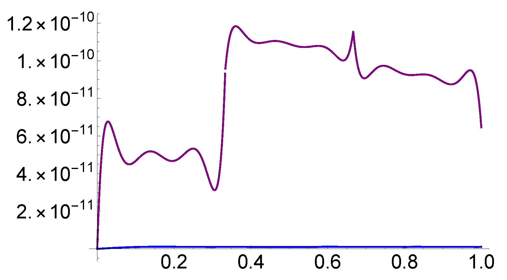
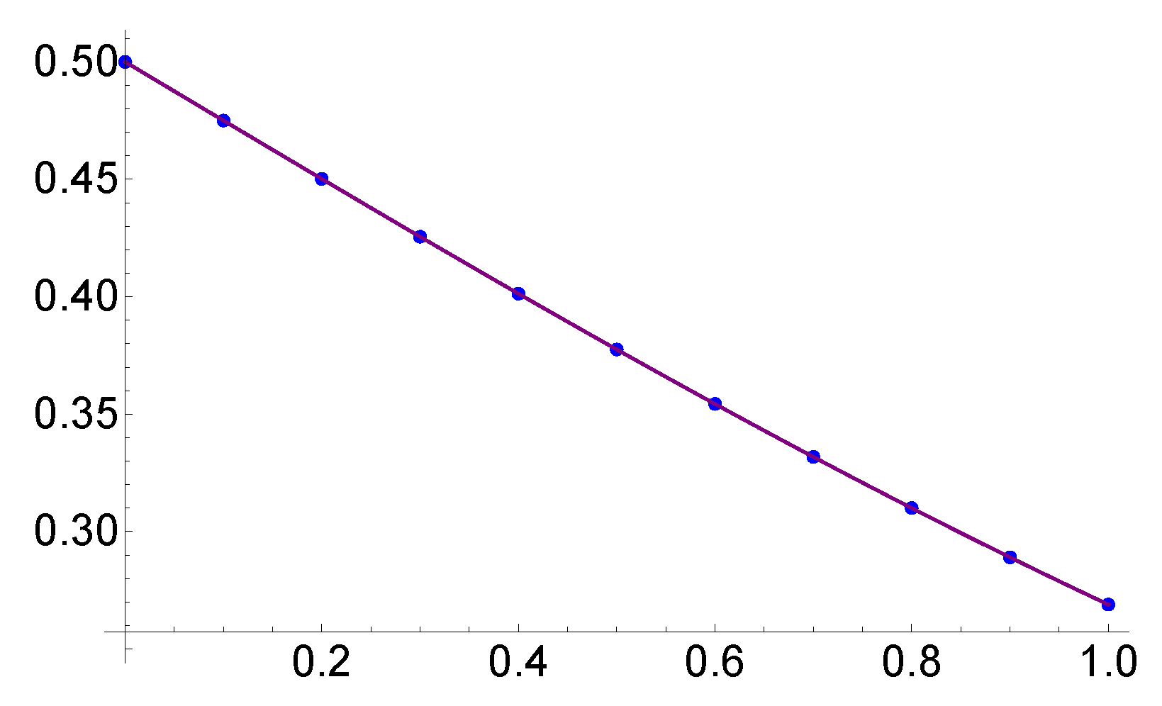
In Figure 1, we make a comparison regarding the absolute errors for $f\left(x\right)$ when $\alpha =1$ (purple) and $\alpha =2$ (blue), and we notice that our method improves the classical method by approximately 11 orders of magnitude. In Figure 2, we compare the exact and the approximate solutions for $q=1$ and $\alpha =2$, and we notice the perfect overlap of the two graphs.

5.2. Example 2

Next, the following equation is considered

$$\begin{array}{c}\hfill D^{q}f\left(x\right)-xf\left(x\right)+2f^2\left(x\right)=g\left(x\right),\mathrm{where}0<q\le 1,0\le x\le 1,\end{array}$$

and

$$\begin{array}{ccc}\hfill g\left(x\right)& =& -x^9+2x^{16}+3x^{5+q/2}-12x^{12+q/2}+\frac{81}{8}x-\frac{9}{4}{x}^{1+q}+27x^{8+q}-27x^{4+3q/2}\hfill \\ & & +\frac{40320}{\mathsf{\Gamma }(9-q)}{x}^{8-q}-\frac{3\mathsf{\Gamma }(5+q/2)}{\mathsf{\Gamma }(5-q/2)}{t}^{4-q/2}+\frac{9\mathsf{\Gamma }(1+q)}{4},\hfill \end{array}$$

which is subjected to the initial condition $f\left(0\right)=0$.

This problem admits the exact solution, which is given by the expression

$$\begin{array}{c}\hfill f\left(x\right)=x^8-3x^{4+q/2}+\frac{9}{4}{x}^q.\end{array}$$

We solve the problem for $N=1$ and $M=8$, with $\alpha =q$. Through

$$D^{q}f\left(x\right)=C^T{B}^{\alpha }\left(x\right),$$

we obtain

$$f\left(x\right)=C^T{\overline{B}}^{\alpha }(x,q),$$

and these results entered into Equation (20) give

$$\begin{array}{c}\hfill C^T{B}^{\alpha }\left(x\right)-x{C}^T{\overline{B}}^{\alpha }(x,q)+2{\left(C^T{\overline{B}}^{\alpha }(x,q)\right)}^2=g\left(x\right).\end{array}$$

(20)

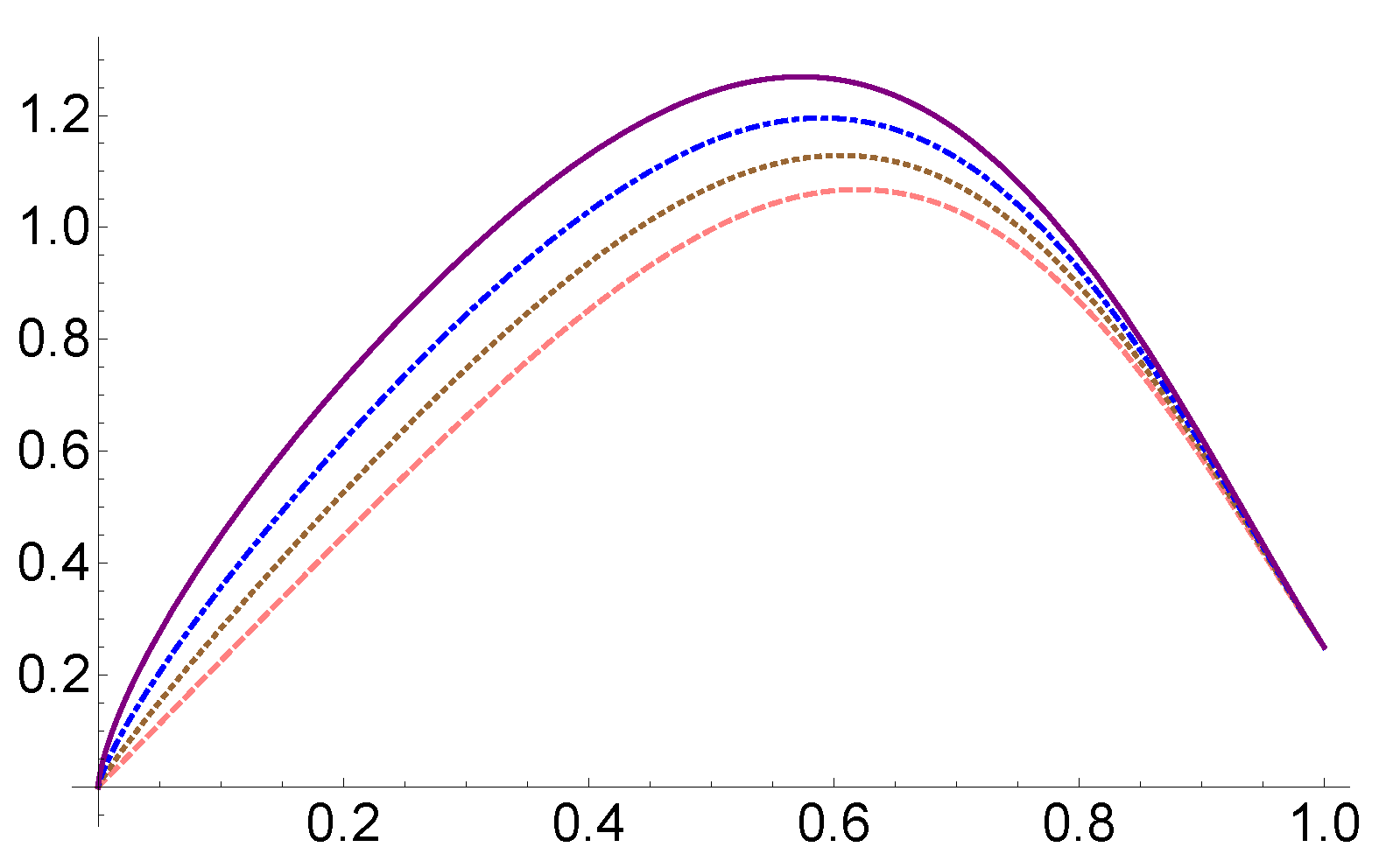
Collocating Equation (20) at Newton–Cotes nodes, we obtain a system of algebraic equations, and the solution of this system gives the constants C. For this setup, we obtain the exact solution when $\alpha =q$. In Figure 3, we graphically represent the numerical solution for $q=\alpha =0.7$ (dashed, opal), $q=\alpha =0.8$ (dotted, brown), $q=\alpha =0.9$ (dashed-dotted, blue), and $q=\alpha =1$ (continuous, purple).

5.3. Example 3

We consider the following example [57,58,59]

$$\begin{array}{c}\hfill D^{q}f\left(x\right)=1-f^2\left(x\right),\mathrm{for}0<q\le 1,0\le x\le 1,\end{array}$$

and

$$\begin{array}{c}\hfill f\left(0\right)=0.\end{array}$$

In the case $q=1$, the exact solution is known

$$\begin{array}{c}\hfill f\left(x\right)=tanhx.\end{array}$$

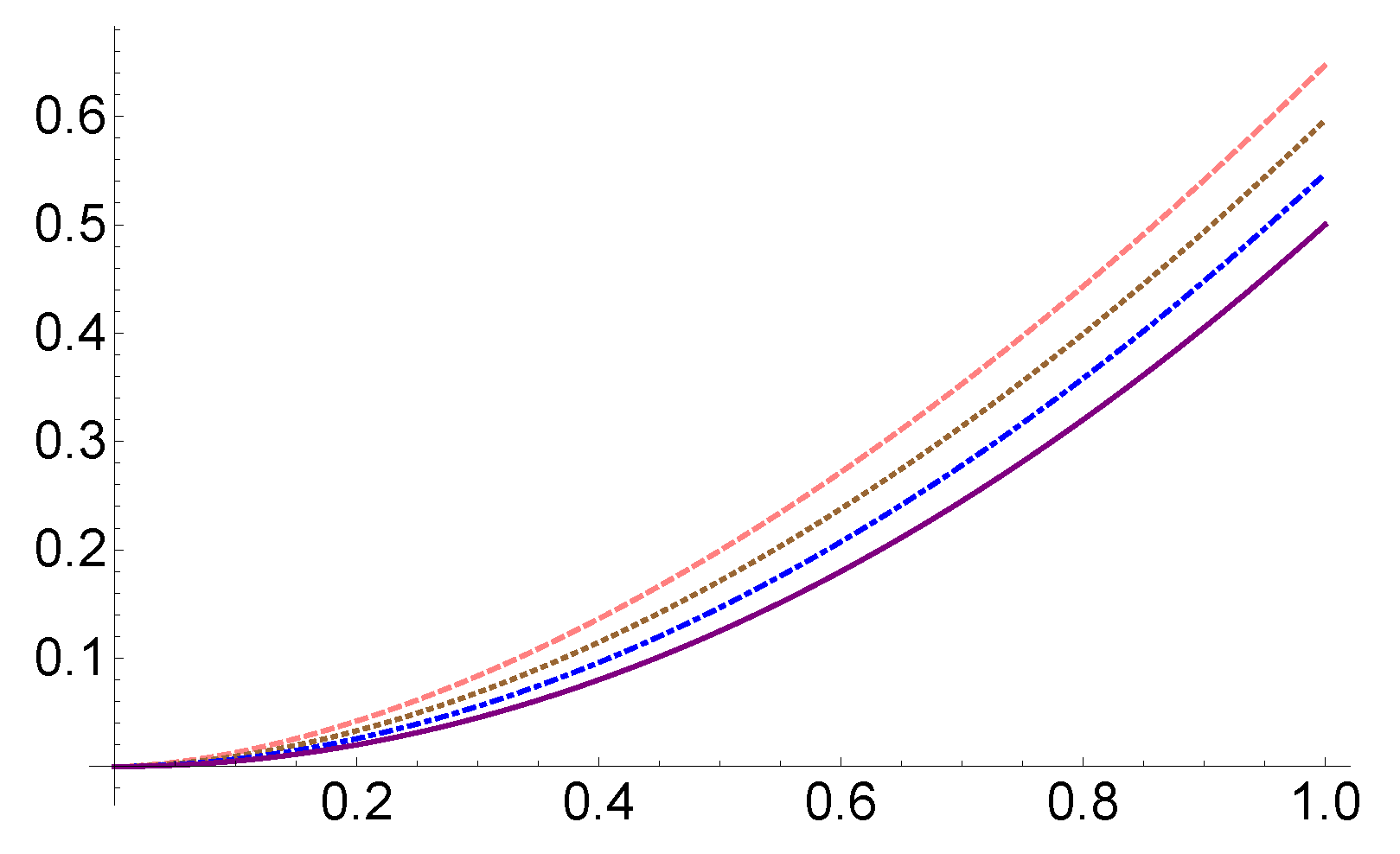
We solve this problem with $N=1$ and $M=11$. We compare the absolute errors of the exact solution obtained by our method with other methods with the same dimension of the base, in

Table 1. Absolute errors for $N=1$ and $M=11$, $q=1$, $\alpha =2$ in Example 3.

x	Method [49]	Method [50]	Method [33]	This Method
0.2	$1.1\times {10}^{-8}$	$3.2\times {10}^{-7}$	$2.7\times {10}^{-10}$	$3.4\times {10}^{-11}$
0.4	$5.4\times {10}^{-6}$	$5.0\times {10}^{-6}$	$2.5\times {10}^{-10}$	$2.9\times {10}^{-11}$
0.6	$1.9\times {10}^{-4}$	$1.9\times {10}^{-4}$	$2.1\times {10}^{-10}$	$2.4\times {10}^{-11}$
0.8	$2.3\times {10}^{-3}$	$2.3\times {10}^{-3}$	$2.9\times {10}^{-10}$	$1.8\times {10}^{-11}$
1.0	$1.6\times {10}^{-2}$	$1.6\times {10}^{-2}$	$6.8\times {10}^{-8}$	$1.5\times {10}^{-11}$

. In Figure 4, we represent the approximate solutions $f\left(x\right)$, $\alpha =q$, with $q=0.7$ (dashed), $q=0.8$ (dotted), $q=0.9$ (dashed-dotted), and exact solution $q=1$ (continuous).

5.4. Example 4

In this example, we solve the equation [22,59]

$$D^{q}f\left(x\right)={\left(\frac{x^{q+1}}{\mathsf{\Gamma }\left(q+2\right)}\right)}^2+x-f^2\left(x\right),0<q\le 1,0\le x\le 1,$$

with

$$f\left(0\right)=0.$$

The solution of this equation is

$$f\left(x\right)=\frac{x^{q+1}}{\mathsf{\Gamma }\left(q+2\right)}.$$

In order to solve this example, we consider $N=1$ and $M=4$, with $\alpha =0.5$. The comparison between our results and the results in [22] for a four-dimensional base are presented in

Table 2. Absolute errors for $N=1$ and $M=4$, $\alpha =0.5$ in Example 4.

x	Method [22]	This Method	Method [22]	This Method
	$\mathit{q}=\mathbf{0}.\mathbf{5}$	$\mathit{q}=\mathbf{0}.\mathbf{5}$	$\mathit{q}=\mathbf{0}.\mathbf{8}$	$\mathit{q}=\mathbf{0}.\mathbf{8}$
0	$8.4\times {10}^{-10}$	0	$5.0\times {10}^{-5}$	0
0.1	$1.4\times {10}^{-9}$	$6.9\times {10}^{-18}$	$6.9\times {10}^{-6}$	$8.6\times {10}^{-18}$
0.2	$1.7\times {10}^{-9}$	$1.3\times {10}^{-17}$	$4.6\times {10}^{-6}$	$6.9\times {10}^{-18}$
0.3	$2.0\times {10}^{-8}$	0	$4.3\times {10}^{-6}$	$1.3\times {10}^{-17}$
0.4	$1.5\times {10}^{-8}$	$2.7\times {10}^{-17}$	$4.2\times {10}^{-6}$	0
0.5	$1.1\times {10}^{-8}$	$5.5\times {10}^{-17}$	$3.4\times {10}^{-5}$	0
0.6	$9.0\times {10}^{-9}$	0	$3.1\times {10}^{-5}$	0
0.7	$7.5\times {10}^{-9}$	0	$3.3\times {10}^{-5}$	$5.5\times {10}^{-17}$
0.8	$7.0\times {10}^{-9}$	0	$5.3\times {10}^{-5}$	$5.5\times {10}^{-17}$
0.9	$7.8\times {10}^{-9}$	$2.2\times {10}^{-16}$	$1.3\times {10}^{-4}$	0
1	$1.0\times {10}^{-8}$	$1.1\times {10}^{-16}$	$3.6\times {10}^{-4}$	0

. The absolute errors for $f\left(x\right)$ for $\alpha =1$ (purple) and $\alpha =2$ (blue) are represented in Figure 5. In conclusion, for this equation, the fractional method is more efficient than the ordinary method. In Figure 6, we represent the approximate solutions for $f\left(x\right)$ with $\alpha =q$, with $q=0.7$ (dashed), $q=0.8$ (dotted), $q=0.9$ (dashed-dotted), and exact solution $q=1$ (continuous).

5.5. Example 5

In this example, we solve the following problem [51]

$$D^{q}f\left(x\right)+f\left(x\right)+f^2\left(x\right)={\left(E_q\left(-x^q\right)\right)}^2,x\in (0,1),0<\alpha <1,$$

with

$$f\left(0\right)=1.$$

The problem has exact solution

$$f\left(x\right)=E_q\left(-x^q\right),$$

where $E_q\left(x\right)$ is the Mittag–Leffler function that has the following definition

$$E_q\left(x\right)=\sum _{k=0}^{\infty }\frac{x^k}{\mathsf{\Gamma }(qk+1)}.$$

We solve this example considering $N=1$ and $M=16$, with $\alpha =q$. The comparison between our results and results [51] with 25 basis elements is presented in

Table 3. Absolute errors for $N=1$ and $M=16$, $\alpha =q$ in Example 5.

$\mathit{\alpha }$	Method [51]	This Method
$0.25$	$1.7\times {10}^{-11}$	$4.2\times {10}^{-12}$
$0.50$	$9.3\times {10}^{-12}$	$1.2\times {10}^{-13}$
$0.75$	$7.4\times {10}^{-12}$	$1.3\times {10}^{-13}$
$0.95$	$3.2\times {10}^{-14}$	$1.1\times {10}^{-14}$

. In Figure 7, we compare the absolute errors for $f\left(x\right)$ with $N=1$ and $M=4$ when $\alpha =0.5$ (purple) and $\alpha =1$ (blue), and in Figure 8, we plot the approximate solutions for $f\left(x\right)$, $\alpha =q$, with $q=0.25$ (dashed), $q=0.5$ (dotted), $q=0.75$ (dashed-dotted), and $q=0.95$ (continuous).

6. Conclusions

In this paper, new functions called fractional-order hybrid functions of block-pulse and Bernoulli polynomials based on Bernoulli polynomials and block functions have been defined. Moreover, we have determined the fractional-order integration and derivative formulas of the fractional-order hybrid functions. Furthermore, making use of the mentioned collocation method and employing the fractional integration operational matrix, we were able to make approximations concerning the solution of the linear and nonlinear initial value problems, which are subjected to a fractional-order q. The benefits of this method are noticeable in Figure 1 and Figure 2: in Figure 1, we illustrate the absolute errors when $\alpha =1$ and $\alpha =2$, reflecting the accuracy of the solutions obtained from the system of algebraic equations, and in Figure 2, we compare the exact and approximate solution for $\alpha =2$ and $q=1$. As a result, we observe that the fractional method is of high accuracy, as, for $\alpha =2$, the absolute error is minimal.

This method consists of the derived Riemann–Liouville fractional integral operator applied for the fractional-order Bernoulli polynomials. The final form of the modified polynomials has a dependency of the incomplete beta function defined in Equation (4). Using this fractional integral operator and the Newton–Cotes nodes for collocation, we determine a system of $N(M+1)$ algebraic equations. In order to solve these equations, we have to use Newton’s iterative method.

Following the direct derivation of the Riemann–Liouville fractional integral operator for a hybrid of block-pulse functions and Bernoulli polynomials, as presented in [46,47,48], the advantages become apparent. This operator is used to reduce to the solution of algebraic equations the solution of the FDEs and systems of FDEs, which helps to solve problems found in engineering and multiple other areas of science.

We considered five examples that clearly indicate the advantages of the current method and illustrate its efficiency. The illustrative examples point towards the conclusion that the presented method is more efficient than the ordinary one. For example, in Figure 5, we present the absolute errors for $f\left(x\right)$ with $\alpha =1$ and $\alpha =2$. Similarly to Example 1, the greater $\alpha$ is, the lower the absolute errors are, which clearly shows the benefits. In correlation to Figure 5, we plotted the approximate solutions shown in Figure 6 when $\alpha =q$, with q taking different values, for $N=1$ and $M=4$. The result indicates that the solutions, based on the necessary approximations, lead to the ordinary solution, being consequently convergent. Figure 3, corresponding to Example 2, also shows that the approximate solutions converge to the ordinary one, thus emphasizing the accuracy of the fractional method.

In Example 3, we show the accuracy of the fractional method, for $N=1$ and $M=11$. Table 1 compares the results of our method with methods [33,49,50]. The accuracy of this method is less than $3.4\times {10}^{-15}$, whereas the other methods present accuracies of $1.6\times {10}^{-2}$, $3.2\times {10}^{-6}$ and $2.9\times {10}^{-10}$, respectively. Table 2, corresponding to Example 4, compares the results of method [22] with our method. Our results have an error of less than $2.2\times {10}^{-16}$ and $5.5\times {10}^{-17}$, compared to errors such as $2.0\times {10}^{-8}$ and $3.6\times {10}^{-4}$ when $q=0.5$ and $q=0.8$, thus indicating that the present method has a higher grade of accuracy than those cited. In the last example, Table 3 shows that our results are of higher accuracy compared to the results determined in [51]. The results obtained with the present method are very accurate, generating errors of less than ${10}^{-11}$ in Examples 1 and 3, ${10}^{-17}$ in 4, and ${10}^{-12}$ in 5.

The numerical method associated with this paper is simple and does not require high complexity in programming. After obtaining these equations, we collocate them in the Newton–Cotes nodes, resulting in a number of $N(M+1)$ algebraic equations. Using Newton’s iterative method, we solve these equations for the vector C.

References

- Oldham, K.B.; Spanier, J. The Fractional Calculus; Academic Press: New York, NY, USA, 1974. [Google Scholar]
- Miller, K.S.; Ross, B. An Introduction to the Fractional Calculus and Fractional Differential Equations; John Wiley: New York, NY, USA, 1993. [Google Scholar]
- Machado, J.T.; Kiryakova, V.; Mainardi, F. Recent history of fractional calculus. Commun. Nonlinear Sci. Numer. Simul. 2011, 16, 1140–1153. [Google Scholar] [CrossRef] [Green Version]
- Bagley, R.L.; Torvik, P.J. Fractional calculus in the transient analysis of viscoelastically damped structures. AIAA J. 1985, 23, 918–925. [Google Scholar] [CrossRef]
- Baillie, R. Long memory processes and fractional integration in econometrics. J. Econom. 1996, 73, 5–59. [Google Scholar] [CrossRef]
- Mainardi, F. Some Basic Problems in Continuum and Statistical Mechanics. In Fractals and Fractional Calculus in Continuum Mechanics; Carpinteri, A., Mainardi, F., Eds.; Springer: New York, NY, USA, 1997. [Google Scholar]
- Rossikhin, Y.; Shitikova, M.V. Applications of fractional calculus to dynamic problems of linear and nonlinear hereditary mechanics of solids. Appl. Mech. Rev. 1997, 50, 15–67. [Google Scholar] [CrossRef]
- Oldham, K.B. Fractional differential equations in electrochemistry. Adv. Eng. Softw. 2010, 41, 9–12. [Google Scholar] [CrossRef]
- Erturk, V.S.; Odibat, Z.M.; Momani, S. An approximate solution of a fractional order differential equation model of human T-cell lymphotropic virus I (HTLV-I) infection of CD4+ T-cells. Comput. Math. Appl. 2011, 62, 996–1002. [Google Scholar] [CrossRef] [Green Version]
- SEl-Wakil, A.; Abulwafa, E.M.; El-shewy, E.K.; Mahmoud, A.A. Time-Fractional KdV Equation Describing the Propagation of Electron-Acoustic Waves in plasma. Comput. Math. Appl. 2011, 62, 996. [Google Scholar]
- Gaul, L.; Klein, P.; Kemple, S. Damping description involving fractional operators. Mech. Syst. Signal. Process. 1991, 5, 81–88. [Google Scholar] [CrossRef]
- Suarez, L.; Shokooh, A. An eigenvector expansion method for the solution of motion containing fractional derivatives. J. Appl. Mech. 1997, 64, 629–635. [Google Scholar] [CrossRef]
- Podlubny, I. Fractional Differential Equations: An Introduction to Fractional Derivatives, Fractional Differential Equations, to Methods of Their Solution and Some of Their Applications; Academic Press: New York, NY, USA, 1998. [Google Scholar]
- Odibat, Z.; Momani, S. Analytical solution of a time-fractional Navier–Stokes equation by Adomian decomposition method. Int. J. Nonlinear Sci. Numer. Simul. 2006, 7, 27. [Google Scholar]
- Meerschaert, M.; Tadjeran, C. Finite difference approximations for two-sided space-fractional partial differential equations. Appl. Numer. Math. 2006, 56, 80–90. [Google Scholar] [CrossRef]
- Daftardar-Gejji, V.; Jafari, H. Solving a multi-order fractional differential equation using Adomian decomposition. Appl. Math. Comput. 2007, 189, 541–548. [Google Scholar] [CrossRef]
- Odibat, Z.; Shawagfeh, N. Generalized Taylor’s formula. Appl. Math. Comput. 2007, 186, 286. [Google Scholar] [CrossRef]
- Abdulaziz, O.; Hashim, I.; Momani, S. Solving systems of fractional differential equations by homotopy-perturbation method. Phys. Lett. A 2008, 372, 451–459. [Google Scholar] [CrossRef]
- Ertrk, V.S.; Momani, S. Solving systems of fractional differential equations using differential transform method. J. Comput. Appl. Math. 2008, 215, 142. [Google Scholar] [CrossRef] [Green Version]
- Hashim, I.; Abdulaziz, O.; Momani, S. Homotopy analysis method for fractional IVPs. J. Commun. Nonlinear Sci. Numer. Simul. 2009, 14, 674–684. [Google Scholar] [CrossRef]
- Bhrawy, A.H.; Tharwat, M.M.; Yildirim, A. A new formula for fractional integrals of Chebyshev polynomials: Application for solving multi-term fractional differential equations. Appl. Math. Model. 2013, 37, 4245–4252. [Google Scholar] [CrossRef]
- Rahimkhani, P.; Ordokhani, Y.; Babolian, E. Fractional-order Bernoulli wavelets and their applications. Appl. Math. Model. 2016, 40, 8087–8107. [Google Scholar] [CrossRef]
- Marzban, H.; Razzaghi, M. Hybrid functions approach for linearly constrained quadratic optimal control problems. Appl. Math. Model. 2003, 27, 471–485. [Google Scholar] [CrossRef]
- Haddadi, N.; Ordokhani, Y.; Razzaghi, M. Optimal control of delay systems by using a hybrid functions approximation. J. Optim. Theory Appl. 2012, 153, 338–356. [Google Scholar] [CrossRef]
- Zhu, L.; Fan, Q. Solving fractional nonlinear Fredholm integro-differential equations by the second kind Chebyshev wavelet. Commun. Nonlinear Sci. Num. Simul. 2012, 17, 2333–2341. [Google Scholar] [CrossRef]
- Heydari, M.H.; Hooshmandasl, M.R.; Mohammadi, F. Legendre wavelets method for solving fractional partial differential equations with Dirichlet boundary conditions. Appl. Math. Comput. 2014, 234, 267–276. [Google Scholar] [CrossRef]
- Saeedi, H.; Moghadam, M.M.; Mollahasani, N.; Chuev, G.N. A CAS wavelet method for solving nonlinear Fredholm integro-differential equations of fractional order. Commun. Nonlinear Sci. Num. Simul. 2011, 16, 1154–1163. [Google Scholar] [CrossRef]
- Li, Y.; Zhao, W. Haar wavelet operational matrix of fractional order integration and its applications in solving the fractional order differential equations. Appl. Math. Comput. 2010, 216, 2276–2285. [Google Scholar] [CrossRef]
- Keshavarz, E.; Ordokhani, Y.; Razzaghi, M. Bernoulli wavelet operational matrix of fractional order integration and its applications in solving the fractional order differential equations. Appl. Math. Model. 2014, 38, 6038–6051. [Google Scholar] [CrossRef]
- Kazem, S.; Abbasbandy, S.; Kumar, S. Fractional-order Legendre functions for solving fractional-order differential equations. Appl. Math. Model. 2013, 37, 5498–5510. [Google Scholar] [CrossRef]
- Yin, F.; Song, J.; Wu, Y.; Zhang, L. Numerical solution of the fractional partial differential equations by the two-dimensional fractional-order Legendre functions. Abstr. Appl. Anal. 2013, 2013, 562140. [Google Scholar] [CrossRef] [Green Version]
- Bhrawy, A.H.; Alhamed, Y.A.; Baleanu, D. New spectral techniques for systems of fractional differential equations using fractional-order generalized Laguerre orthogonal functions. Fract. Calc. Appl. Anal. 2014, 17, 1138. [Google Scholar] [CrossRef]
- Yuzbasi, S. Numerical solutions of fractional Riccati type differential equations by means of the Bernstein polynomials. Appl. Math. Comput. 2013, 219, 6328. [Google Scholar] [CrossRef]
- Chen, Y.; Sun, Y.; Liu, L. Numerical solution of fractional partial differential equations with variable coefficients using generalized fractional-order Legendre functions. Appl. Math. Comput. 2014, 244, 847. [Google Scholar] [CrossRef]
- Rahimkhani, P.; Ordokhani, Y.; Babolian, E. An efficient approximate method for solving delay fractional optimal control problems. Nonlinear Dyn. 2016, 86, 1649–1661. [Google Scholar] [CrossRef]
- Rahimkhani, P.; Ordokhani, Y.; Babolian, E. A new operational matrix based on Bernoulli wavelets for solving fractional delay differential equations. Numer. Algorithms 2017, 74, 223. [Google Scholar] [CrossRef]
- Rahimkhani, P.; Ordokhani, Y.; Babolian, E. Numerical solution of fractional pantograph differential equations by using generalized fractional-order Bernoulli wavelet. J. Comput. Appl. Math. 2017, 309, 493. [Google Scholar] [CrossRef]
- Rahimkhani, P.; Ordokhani, Y.; Babolian, E. Fractional-order Bernoulli functions and their applications in solving fractional Fredholem–Volterra integro-differential equations. Appl. Numer. Math. 2017, 122, 66. [Google Scholar] [CrossRef]
- Razzaghi, M.; Marzban, H.R. Direct method for variational problems via hybrid of block-pulse and Chebyshev functions. Math. Probl. Eng. 2000, 6, 85. [Google Scholar] [CrossRef]
- Wang, X.T.; Li, Y.M. Numerical solutions of integrodifferential systems by hybrid of general block-pulse functions and the second Chebyshev polynomials. Appl. Math. Comput. 2009, 209, 266. [Google Scholar] [CrossRef] [Green Version]
- Razzaghi, M.; Marzban, H.R. A hybrid analysis direct method in the calculus of variations. Int. J. Comput. Math. 2000, 75, 259. [Google Scholar] [CrossRef]
- Singh, V.K.; Pandey, R.K.; Singh, S. A stable algorithm for Hankel transforms using hybrid of Block-pulse and Legendre polynomials. Comput. Phys. Commun. 2010, 181, 1–10. [Google Scholar] [CrossRef]
- Marzban, H.R.; Razzaghi, M. Analysis of time-delay systems via hybrid of block-pulse functions and Taylor series. J. Vib. Control. 2005, 11, 1455. [Google Scholar] [CrossRef]
- Marzban, H.R.; Razzaghi, M. Solution of multi-delay systems using hybrid of block-pulse functions and Taylor series. J. Sound Vib. 2006, 292, 954. [Google Scholar] [CrossRef]
- Mashayekhi, S.; Ordokhani, Y.; Razzaghi, M. Hybrid functions approach for nonlinear constrained optimal control problems. Commun. Nonlinear Sci. Numer. Simul. 2012, 17, 1831–1843. [Google Scholar] [CrossRef]
- Mashayekhi, S.; Razzaghi, M. Numerical solution of nonlinear fractional integro-differential equations by hybrid functions. Eng. Anal. Bound. Elem. 2015, 56, 81–89. [Google Scholar] [CrossRef]
- Mashayekhi, S.; Razzaghi, M. Numerical solution of distributed order fractional differential equations by hybrid functions. J. Comput. Phys. 2016, 315, 169–181. [Google Scholar] [CrossRef]
- Mashayekhi, S.; Razzaghi, M. Numerical solution of the fractional Bagley-Torvik equation by using hybrid functions approximation. Math. Method. Appl. Sci. 2016, 39, 353–365. [Google Scholar] [CrossRef]
- Momani, S.; Qaralleh, R. An efficient method for solving systems of fractional integro-differential equations. Comput. Math. Appl. 2006, 52, 459–470. [Google Scholar] [CrossRef] [Green Version]
- Odibat, Z.M.; Momani, S. Modified homotopy perturbation method: Application to quadratic Riccati differential equation of fractional order. Chaos Solitons Fract. 2008, 36, 167–174. [Google Scholar] [CrossRef]
- Kashkari, B.S.H.; Syam, M.I. Fractional-order Legendre operational matrix of fractional integration for solving the Riccati equation with fractional order. Appl. Math. Comput. 2016, 290, 281–291. [Google Scholar] [CrossRef]
- Rehman, M.U.; Khan, R.A. A numerical method for solving boundary value problems for fractional differential equations. Appl. Math. Model. 2012, 36, 894–907. [Google Scholar] [CrossRef]
- Costabile, F.; Dell’Accio, F.; Gualtieri, M.I. A new approach to Bernoulli polynomials. Rend. Mat. Ser. VII 2006, 26, 112. [Google Scholar]
- Arfken, G. Mathematical Methods for Physicists; Academic Press: San Diego, CA, USA, 1985. [Google Scholar]
- Postavaru, O.; Toma, A. Numerical solution of two-dimensional fractional-order partial differential equations using hybrid functions. Partial. Differ. Equ. Appl. Math. 2021, 4, 100099. [Google Scholar] [CrossRef]
- Postavaru, O.; Toma, A. A numerical approach based on fractional-order hybrid functions of block-pulse and Bernoulli polynomials for numerical solutions of fractional optimal control problems. Math. Comput. Simul. 2022, 194, 269–284. [Google Scholar] [CrossRef]
- Bota, C.; Caruntu, B. Analytical approximate solutions for quadratic Riccati differential equation of fractional order using the Polynomial Least Squares Method. Chaos Solitons Fractals 2017, 102, 339–345. [Google Scholar] [CrossRef]
- Singh, H.; Srivastava, H. Jacobi collocation method for the approximate solution of some fractional-order Riccati differential equations with variable coefficients. Physica A 2019, 523, 1130–1149. [Google Scholar] [CrossRef]
- Mohammadi, F.; Cattani, C. A generalized fractional-order Legendre wavelet Tau method for solving fractional differential equations. J. Comput. Appl. Math. 2018, 339, 306–316. [Google Scholar] [CrossRef]
Figure 1.
Absolute errors for , (purple) and (blue), for Example 1.
Figure 2.
Exact and approximate solutions in Example 1, for and .
Figure 3.
with , where (dashed), (dotted), (dashed-dotted), and exact solution (continuous), for Example 2.
Figure 4.
, where (dashed), (dotted), (dashed-dotted), and exact solution (continuous), with , for Example 3.
Figure 5.
The absolute errors for for (purple) and (blue), for Example 4.
Figure 6.
, where (dashed), (dotted), (dashed-dotted), and exact solution (continuous), with , for Example 4.
Figure 7.
The absolute errors for for (purple) and (blue), for Example 5.
Figure 8.
, where (dashed), (dotted), (dashed-dotted), and (continuous), with , for Example 5.