Financial Applications on Fractional Lévy Stochastic Processes

Abstract

In this present work, we perform a numerical analysis of the value of the European style options as well as a sensitivity analysis for the option price with respect to some parameters of the model when the underlying price process is driven by a fractional Lévy process. The option price is given by a deterministic representation by means of a real valued function satisfying some fractional PDE. The numerical scheme of the fractional PDE is obtained by means of a weighted and shifted Grunwald approximation.

1. Introduction and Notations

The pricing of financial instruments is a problem of significant interest for risk management and hedging and/or in trading derivatives expecting more income in finance industries. Financial instruments are linked to underlying assets whose dynamics are modeled by an exponential of a Lévy process of the form

$$d(log{S}_t)=(\mu -\frac{1}{2}{\sigma }^2)dt+\sigma d{L}_t,$$

(1)

under the risk neutral measure Q, where $\mu >0$ is the average compounded growth of the stock $S_t$, $d{L}_t$ is the increment of Lévy and $\sigma$ is the volatility of the risky asset, induced by Lévy jump. We refer to Raible (2000) [1], Schoutens [2] (2003) and Eberlein (2014) [3] and the references therein for more details on non-fractional Lévy models in finance. It is well known that the distribution of a Lévy process is characterized by its characteristic function, which is given by the Lévy–Khintchine formula. We can characterize the Lévy when a $L_t$ dependent random variable with time is a Lévy process if and only if it has independent stationary increments with an exponential characteristic function given by the so-called Lévy–Khintchine representation. Indeed, if ${\left(L_t\right)}_{t\ge 0}$ is a Lévy process on $\mathbb{R}$ with characteristic triplet $(m,\sigma ,\nu )$, then $\mathbb{E}\left[e^{i\varpi L_t}\right]=e^{t\psi \left(\varpi \right)},t\in \mathbb{R}$. The function $\psi$ is called the characteristic exponent and can be expressed as

$$\psi \left(\varpi \right)=im\varpi +\frac{{\sigma }^2}{2}{\left(i\varpi \right)}^2+{\int }_{-\infty }^{\infty }(e^{i\varpi \kappa }-1-i\varpi {\mathrm{I}}_{\left|\kappa \right|<1})\nu \left(d\kappa \right),$$

(2)

where $m\in \mathbb{R}$, $\sigma \ge 0$ and $\nu$ is the Lévy measure that controls the jumps such that ${\int }_{\mathbb{R}}min\left(1,{\kappa }^2\right)\nu \left(d\kappa \right)$ is finite and ${\mathrm{I}}_A$ is the indicator function defined by

$${\mathrm{I}}_A\left(x\right):=\left\{\begin{array}{cc}1& \mathrm{if}x\in A\\ 0& \mathrm{otherwise}.\end{array}\right.$$

An Example of a Lévy Process: Lévy Stable Processes (LSP)

Let $L_t^{\alpha ,\beta }$ be a Lévy $\alpha$-stable process with skew parameter $\beta$ and stability index $\alpha$. We shall take $\beta =-1$ and assume that $1<\alpha <2$. Consequently, for each $n>0$ and $0<t<T$,

$$\mathbb{E}\left[exp,\left(n,\sigma ,L_t^{\alpha ,-1}\right)\right]=exp\left(-t{n}^{\alpha }{\sigma }^{\alpha }sec\left(\frac{\pi \alpha }{2}\right)\right)<+\infty .$$

Recall that the density function ${\nu }_{LS}\left(x\right)=\frac{\nu \left(dx\right)}{dx}$ of the stable Lévy process with $\alpha \in (0,2)$ is given by

$${\nu }_{LS}\left(x\right)=\left\{\begin{array}{cc}\frac{ad}{{\left|x\right|}^{1+\alpha }}& \mathrm{for}x<0,\\ \frac{bd}{x^{1+\alpha }}& \mathrm{for}x>0\end{array}\right.$$

where $1=a+b$ and $d>0$. Substituting the above density in Equation (2) yields the characteristic exponent of a LSP with $\beta =a-b$

$${\psi }_{LS}\left(\varpi \right)=i\varpi m-\frac{{\sigma }^{\alpha }{\left|\varpi \right|}^{\alpha }}{2}\times [1-i\beta tan\left(\frac{\alpha \pi }{2}\right)sign\left(\varpi \right)].$$

An equivalent from of ${\psi }_{LS}\left(\varpi \right)$ is given below

$${\psi }_{LS}\left(\varpi \right)=i\varpi m-\frac{{\sigma }^{\alpha }}{4cos\left(\frac{\alpha \pi }{2}\right)}[{\left(i\varpi \right)}^{\alpha }(1-\beta )+{(-i\varpi )}^{\alpha }(1+\beta )]$$

where the condition $\beta =-1$, yield $a=0$ and $b=1$ (see Cartea et al. [4] for more details), hence

$${\psi }_{LS}\left(\varpi \right)=i\varpi m-\frac{1}{4cos\left(\frac{\alpha \pi }{2}\right)}{\sigma }^{\alpha }\left[\left(2\right){\left(i\varpi \right)}^{\alpha }\right].$$

(3)

The price of an European call option may be expressed as the risk-neutral conditional expectation

$$V(S_t,t)=e^{-r(T-t)}{\mathbb{E}}^Q[max(S_T-K,0)|{\mathcal{F}}_t],$$

and the value of an European put option may be expressed as the risk-neutral conditional expectation

$$V(S_t,t)=e^{-r(T-t)}{\mathbb{E}}^Q[max(K-S_T,0)|{\mathcal{F}}_t],$$

where the price of the stock follows the dynamic (1) and ${\mathcal{F}}_t$ is the completed and right continuous natural filtration associated to the Lévy stable process. Other extensions to this result have been done in many directions; see Abouagwa and Li [5] (2019) and also Wu et al. [6] (2021).

Our contribution in this paper is to perform a numerical analysis of the value of the European style options as well as a sensitivity analysis for the option price with respect to the model parameters. Numerical methods have been studied using a finite difference scheme for non-fractional jump diffusion and exponential Lévy models for option pricing by Cont and Voltchkova [7] (2005). For the sensitivity analysis, we shall focus mainly on the very well-known Greeks (Delta, Gamma and Vega) and refer to a relatively recent paper by Shokrollahi et al. [8] (2015).

The rest of the article is structured as follows: Section 2 is devoted to the stochastic model we are interested in as well as the deterministic representation of the option price by a real valued function satisfying some fractional PDEs. Section 3 presents the numerical scheme used to discretize the fractional PDE by means of the weighted and shifted Grunwald approximation. Section 4 deals with a numerical implementation to solve the fractional diffusion equation. Moreover, a subsection concerning the numerical computations of Greek parameters giving some information about sensitivity analysis is added.

2. The Stochastic Model and Deterministic Representation

The dynamic of the stock price driven by the $\alpha$-stable Lévy process $L_t^{\alpha ,-1}$ with additional impact term is given for each $0\le t<T$ by the following equation:

$$d^{\gamma }{S}_t=S_t\left((r-q)d{t}^{\gamma }+\sigma d{L}_t^{\alpha ,-1}\right)+\lambda S_{t}d{\beta }_t^{\gamma },S_0\mathrm{initial}\mathrm{price},$$

(4)

where $0<\gamma <1$ and $1<\alpha \le 2$, ${\beta }_t^{\gamma }$ is the number of shares of the stock at time t and the term $\lambda d{\beta }_t^{\gamma }$ ($\lambda \ge 0$) stands for the impact price of the investor’s trading strategy (see Chen et al. (2014) [9] for more details and specific parameters).

Throughout this paper, we only consider trading strategies that can be written in the following form

$$d{\beta }_t^{\gamma }=\eta d{t}^{\gamma }+\zeta d{L}_t^{\alpha ,-1},$$

(5)

with initial number of shares ${\beta }_0^{\gamma }$ and some constants $\eta ,\zeta$. A self-financing strategy ${\left({\theta }_t,{\beta }_t^{\gamma }\right)}_{t\ge 0}$ represented by the wealth process ${\left(V_t\right)}_{t\ge 0}$ for trader is given by

$$V_t={\theta }_t{S}_t^0+{\beta }_t^{\gamma }{S}_t=V_0+{\int }_0^t{\theta }_{u}d{S}_u^0+{\int }_0^t{\beta }_u^{\gamma }d{S}_u,$$

where

$$d{S}_t^0=r{S}_t^{0}dt,S_0^0=1.$$

According to the recent paper by Aljedhi and Kılıçman (2020) [10], the wealth process ${\left(V_t\right)}_{t\ge 0}$ can be written as $V_t=u(S_t,t)$ where $u(x,t)$ is the solution of the fractional partial differential equation (FPDE)

$$\frac{{\partial }^{\gamma }u(x,t)}{\partial t^{\gamma }}+A\frac{\partial u(x,t)}{\partial x}+B\frac{{\partial }^{\alpha }u(x,t)}{\partial x^{\alpha }}=ru(x,t),$$

(6)

under the conditions $u(x,0)=h\left(x\right)$, and $u_t(x,0)=f\left(x\right)$. Here, A and B are constants and their expressions are $A=r-q+\lambda \eta +\frac{{\sigma }^{\alpha }}{2}sec\left(\frac{\alpha \pi }{2}\right)$ and $B=\frac{{\sigma }^{\alpha }}{2}sec\left(\frac{\alpha \pi }{2}\right)$.

Notice also that based on the martingale pricing approach under a risk neural probability measure, $u(S_t,t)$ can be represented as

$$u(S_t,t)={\mathbb{E}}^Q\left[\varphi \left(S_T\right)\right|{\mathcal{F}}_t],$$

where

$$\varphi \left(x\right):=\left\{\begin{array}{cc}\mathrm{European}\mathrm{call}\mathrm{option},& {(x-K)}^{+}\\ \mathrm{European}\mathrm{put}\mathrm{option},& {(K-x)}^{+}.\end{array}\right.$$

The first goal of this paper is to find numerical values of the price of European-style option, based on implicit scheme for the (FPDE) (6) and the Euler–Maruyama scheme for the (4). The second goal is to study the sensitivity of these European options while parameters of the model change.

In our numerical analysis, we combine the method of Demirci et al. (2012) [11] and the method adopted by Shen et al. (2012) [12] to solve our fractional partial differential equation. In particular, in [11], they dealt with Caputo partial differential equations with an initial condition of the form

$$D^{\gamma }y\left(t\right)=g(y\left(t\right),t),y\left(0\right)=y_0.$$

It can be solved as a solution $y_{*}\left(\omega \right)$ to a non-fractional differential equation

$$y\left(t\right)=y_{*}\left(\frac{t^{\gamma }}{\mathrm{\Gamma }(\gamma +1)}\right).$$

Moreover, Jumarie (2010) [13] solved the equation,

$$dy=g\left(t\right)d{t}^{\alpha },t\ge 0,0<\alpha \le 1,y\left(0\right)=y_0,$$

where the integral of $d{t}^{\alpha }$ has the form

$${\int }_0^{t}g\left(x\right)d{x}^{\alpha }=\alpha {\int }_0^t{(t-x)}^{\alpha -1}g\left(x\right)dx$$

(7)

and have used the expression

$$d^{\alpha }x=\mathrm{\Gamma }(1+\alpha )dx.$$

Based on our specific structure of the strategy described in (5), the dynamic of the stock price process (4) becomes

$$d^{\gamma }{S}_t=S_t\left((r-q)d{t}^{\gamma }+\sigma d{L}_t^{\alpha ,-1}\right)+\lambda S_t({\eta }_{t}d{t}^{\gamma }+{\zeta }_{t}d{L}_t^{\alpha ,-1}).$$

(8)

It is well known that, using Itô’s formula to $x_t=log{S}_t$, the (8) has a solution that can be written as

$$x_T=x_{t}exp\left(\frac{{\left(\tau \right)}^{\gamma }}{\mathrm{\Gamma }(1+\gamma )}(r-\mu \lambda \eta -q)+{\int }_t^T(\sigma +\lambda {\zeta }_t)d{L}_u^{\alpha ,-1}\right),$$

(9)

where $\tau =T-t$. We shall use the Euler–Maruyama scheme to find some realizations of the price process and then obtain some simulations of the underlying asset described in Equation (9) by means of the following discrete scheme for $1<\alpha \le 2$:

$$x_{n+1}=x_n+{\upsilon }_{n+1}\frac{{\left({\tau }_{n+1}\right)}^{\gamma }}{\mathrm{\Gamma }(1+\gamma )}(r-q+\lambda \eta -m)+{\upsilon }_{n+1}^{\frac{1}{\alpha }}(\sigma +\lambda \zeta )L_{n+1}^{\alpha ,-1},$$

(10)

where $x_0=log{S}_0$, $t_n=\frac{nT}{N}$ for $n=0,\dots ,N$, ${\tau }_{n+1}=T-t_{n+1}$, ${\upsilon }_{n+1}={\displaystyle \frac{{\sigma }^{\alpha }}{2}}sec\left(\frac{\alpha \pi }{2}\right)$ and $L_{n+1}^{\alpha ,-1}=L_{t_{n+1}}^{\alpha ,-1}-L_{t_n}^{\alpha ,-1}$.

3. Numerical Discretization of the Fractional PDE

The price of the call or put European option associated to the underlying asset governed by the (9) is given by

$$u(S_t,t)={\mathbb{E}}^Q\left[h\left(S_T\right)\right|{\mathcal{F}}_t],$$

where $u(x,t)$ is the solution to the Fractional PDE ($0\le \alpha ,\gamma \le 2$)

$$\frac{{\partial }^{\gamma }u(x,t)}{\partial t^{\gamma }}=A\frac{\partial u(x,t)}{\partial x}+B\frac{{\partial }^{\alpha }u(x,t)}{\partial x^{\alpha }}+ru(x,t)$$

(11)

with the conditions $u(x,0)=h\left(x\right)$, and $u_t(x,0)=f\left(x\right)$. Here A and B are constants, and their expressions are

$$A=r-q+\lambda \eta +\frac{{\sigma }^{\alpha }}{2}sec\left(\frac{\alpha \pi }{2}\right),B=\frac{{\sigma }^{\alpha }}{2}sec\left(\frac{\alpha \pi }{2}\right).$$

We shall use the finite difference method using the shifted Grunwald approximation of the fractional derivative. To do this, we will be working with the notation $u_i^n=u(x_{min}+ih,n\tau )$ with h as the step-size of the space variable and $\tau$ as the step-size of the time variable $i=0,\dots ,N_x$ and $n=1,\dots ,N_t$. We consider now (11) at $(x_i,t_n)$, one gets:

$$\frac{{\partial }^{\gamma }{u}_i^n}{\partial t^{\gamma }}=A\frac{\partial u_i^n}{\partial x}+B\frac{{\partial }^{\alpha }{u}_i^n}{\partial x^{\alpha }}+r{u}_i^n.$$

(12)

Before we move on to the method itself, we should first recall the definition for the Caputo time-fractional derivative [12] as

$$\begin{array}{cc}\hfill \frac{{\partial }^{\gamma }u(x,t_{n+1})}{\partial t^{\gamma }}& =\frac{1}{\mathrm{\Gamma }(1-\gamma )}\sum _{k=0}^n{\int }_{t_k}^{t_{k+1}}\frac{\frac{\partial u}{\partial \eta }(x,\eta )}{{(t_n-\eta )}^{\gamma }}d\eta \hfill \\ & =\frac{1}{\mathrm{\Gamma }(1-\gamma )}\sum _{k=0}^n\frac{u(x,t_{n+1})-u(x,t_k)}{\tau }{\int }_{t_k}^{t_{k+1}}\frac{d\eta }{{(t_n-\eta )}^{\gamma }}+\mathcal{O}\left({\tau }^{2-\gamma }\right)\hfill \\ \hfill & =\frac{{\tau }^{-\gamma }}{\mathrm{\Gamma }(2-\gamma )}\sum _{k=0}^n{b}_k^{\gamma }[u(x,t_{n+1-k})-u(x,t_{n-k})]+\mathcal{O}\left({\tau }^{2-\gamma }\right)\hfill \end{array}$$

where the weights $b_k^{\gamma }$ satisfy the following formula

$$\begin{array}{c}\hfill b_k^{\gamma }={(k+1)}^{\gamma }-k^{1-\gamma },b_0^{\gamma }=1,k=0,1,\cdots ,n.\end{array}$$

For the Riemann–Liouville space derivative with the weighted and shifted Grunwald approximation [14,15], we use

$$\begin{array}{cc}\hfill \frac{{\partial }^{\alpha }u(x,t)}{\partial x^{\alpha }}& =\frac{1}{h^{\alpha }}\sum _{k=0}^m{\omega }_k^{\alpha }u(x,t_{m-k})+\mathcal{O}\left(h\right),\hfill \end{array}$$

where the Grünwald–Letnikov weights ${\omega }_k^{\alpha }={(-1)}^k\left[\begin{array}{c}\alpha \\ k\end{array}\right]$, $k\ge 0$ are the coefficients of the power series of the generating function ${(1-z)}^k=\sum _{k=0}^{\infty }{\omega }_k^{\alpha }{z}^k$. These coefficients satisfy the recursive formula

$$\begin{array}{cc}\hfill {\omega }_k^{\alpha }& =\left(1-\frac{\alpha +1}{k}\right){\omega }_{k-1}^{\alpha },{\omega }_0^{\alpha }=1,k=1,\cdots ,m.\hfill \end{array}$$

Hence, the numerical scheme of (12) is given by

$$\frac{{\tau }^{-\gamma }}{\mathrm{\Gamma }(2-\gamma )}\sum _{k=0}^{n-1}{b}_{n-k-1}^{\gamma }\left(u_k^{i+1}-u_k^i\right)=\frac{A}{2h}\left(u_{i+1}^n-u_{i-1}^n\right)+\frac{B}{h^{\alpha }}\sum _{k=1}^{i+1}{\omega }_k^{\alpha }{u}_{i-k+1}^n+r{u}_i^n.$$

(13)

where

$$\begin{array}{cc}\hfill b_k^{\gamma }& ={(k+1)}^{\gamma }-k^{1-\gamma },b_0^{\gamma }=1,\hfill \\ \hfill {\omega }_k^{\alpha }& =\left(1-\frac{\alpha +1}{k}\right){\omega }_{k-1}^{\alpha },w_0^{\alpha }=1.\hfill \end{array}$$

By developing the left side of the Equation (13), one gets

$$\frac{{\tau }^{-\gamma }}{\mathrm{\Gamma }(2-\gamma )}\left(u_i^n-\sum _{k=1}^{n-1}(b_{n-k-1}^{\gamma }-b_{n-k})u_i^k-b_{n-1}{u}_i^0\right)=\frac{A}{2h}\left(u_{i+1}^n-u_{i-1}^n\right)+\frac{B}{h^{\alpha }}\sum _{k=1}^{i+1}{\omega }_k^{\alpha }{u}_{i-k+1}^n+r{u}_i^n.$$

(14)

Rearranging and substituting $u_i^n$ in Equation (14) by its numerical approximation $U_i^n$, one obtains for $i\in \{1,\dots ,N_x-1\}$ and $n\in \{1,\dots ,N_t-1\}$:

$$U_i^n-{\mu }_1\left(U_{i+1}^n-U_{i-1}^n\right)-{\mu }_2\sum _{k=1}^{i+1}{\omega }_k^{\alpha }{U}_{i-k+1}^n={\mu }_3\sum _{k=1}^{n-1}(b_{n-k-1}^{\gamma }-b_{n-k})U_i^k+{\mu }_0{U}_i^0,$$

(15)

$$U_0^n=u(x_0,t_n),U_{N_x}^n=u(x_{N_x},t_n),$$

(16)

where

$${\mu }_0={\displaystyle \frac{b_{n-1}{\tau }^{\gamma }\mathrm{\Gamma }(2-\gamma )}{1-r\mathrm{\Gamma }(2-\gamma )}},{\mu }_1={\displaystyle \frac{{\tau }^{\gamma }A\mathrm{\Gamma }(2-\gamma )}{2h(1-r\mathrm{\Gamma }(2-\gamma \left)\right)}},$$

and

$${\mu }_2={\displaystyle \frac{{\tau }^{\gamma }B\mathrm{\Gamma }(2-\gamma )}{h^{\alpha }(1-r\mathrm{\Gamma }(2-\gamma ))}},{\mu }_3={\displaystyle \frac{1}{1-r{\tau }^{\gamma }\mathrm{\Gamma }(2-\gamma )}}.$$

In order to develop the numerical result, we must write Equation (15) in matrix form $M{U}^n=U^{n-1}$, which is completed with boundary conditions (16). We note that, unlike in integer-order PDEs, the coefficient matrix M is a square matrix of size $N_x$, and will not be tri-diagonal, which will slow down our numerical algorithm quite significantly. This is due to the non-local nature of the time-fractional and space-fractional derivatives. The structure of M is described in the following way, for $i=1,\dots ,N_x-2$ and $j=1,\dots ,N_x-2$

$$\begin{array}{c}\hfill M_{i,j}=\left\{\begin{array}{cc}-{\mu }_2{\omega }_{i-j+1}^{\alpha }\hfill & ifj<i-1\hfill \\ -{\mu }_1-{\mu }_2{\omega }_2^{\alpha }\hfill & ifj=i-1\hfill \\ 1-{\mu }_2{\omega }_1^{\alpha }\hfill & ifj=i\hfill \\ -{\mu }_1-{\mu }_2{\omega }_0^{\alpha }\hfill & ifj=i+1\hfill \\ 0\hfill & ifj>i+1\hfill \end{array}\right.\end{array}$$

To complete this matrix with the boundary conditions, we have that $M_{0,0}=1$, $M_{0,j}=0$ for $j=1,\dots ,N_x-1$, $M_{N_x-1,N_x-1}=1$, $M_{N_x-1,j}=0$ for $j=1,\dots ,N_x-1$ and the second member is given by

$$\begin{array}{c}\hfill U_i^{n-1}={\mu }_3\sum _{k=1}^{n-1}(b_{n-k-1}^{\gamma }-b_{n-k})U_i^k+{\mu }_0{U}_i^0.\end{array}$$

Now, all we have to deal with are the boundary conditions. For European-type options, the behavior of numerical scheme is similar regardless of performing call and put options. However, in the context of our Lévy stable model, this is not the case. Hence, we describe each case separately.

• For a call option, the payoff is defined by ${\mathrm{\Pi }}_T=\max (S_T-K,0)$. Since we must truncate the spatial domain in order to make it workable from a numerical point of view, we will use the following boundary conditions $u(x_{min},t)=0$ and $u(x_{max},t)=e^{x_{max}}-K{e}^{-r(T-t)}$ where $x_{min}=-log\left(4K\right)$ and $x_{max}=log\left(4K\right)$.
• For a put option, the payoff is defined by ${\mathrm{\Pi }}_T=max(K-S_T,0)$ and we will use the following conditions $u(x_{max},t)=0$ and $u(x_{min},t)=K{e}^{-r(T-t)}-e^{x_{min}}$ where $x_{min}=-log\left(4K\right)$ and $x_{max}=log\left(4K\right)$.

4. Numerical Simulations and Discussions

In this section, we present some numerical simulations in order to validate the stochastic model with associated partial differential equations and illustrate the utility of the novel model. In addition, we compute the price of call and put options in order see the difference with the classical Black and Schole’s price. Finally, we perform the sensitivity analysis, usually applied by financial engineers, that provide useful information for the investors. To this end, we use the parameter settings reported in

Table 1. Parameters’ value.

${\mathit{S}}_0$	Strike K	r	q	$\mathit{\lambda }$	$\mathit{\eta }$	m	$\mathit{\sigma }$	$\mathit{\beta }$	$\mathit{\alpha }$
100	80	$0.02$	1	10	$0.01$	$0.02$	$0.15$	$-1$	$1.76$

for the one-year option.

Under the risk neutral equivalent probability measure and thanks to the martingale property, the value of an option at the present time can be represented as

$$u(S_t,t)={\mathbb{E}}^Q\left[{(K-S_T)}^{+}\right|{\mathcal{F}}_t)]$$

(17)

that is the conditional expected value of the discounted payoff under a chosen risk neutral measure with respect to the all the information available in the market up to time t. This representation allows us to use Monte Carlo techniques to estimate values of the option price by simulating a large number of sample values of $S_T$. Notice that this method uses the risk-neutral valuation approach, which means that one has to take $m=r$.

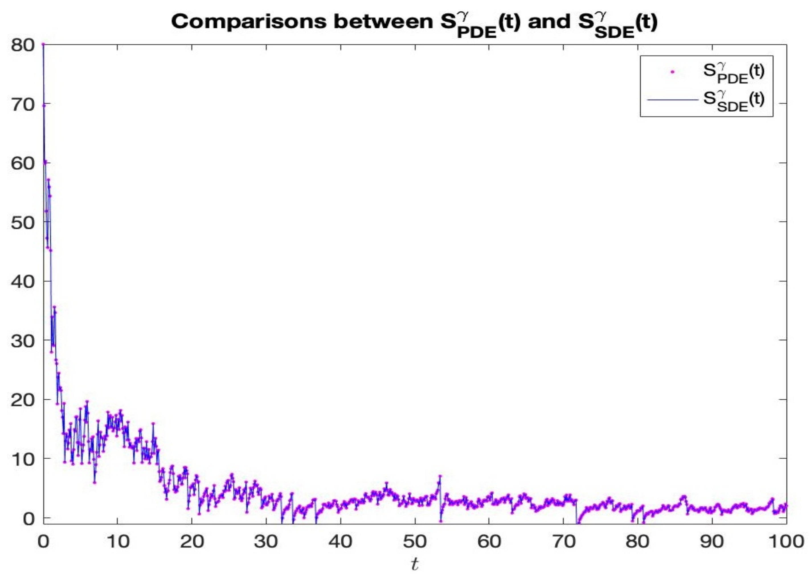
In order to compare the numerical solutions using others numerical computations, we use the Euler–Maruyama method for stochastic differential equation associated with our Lévy stable process. However, the numerical solution of the FPDE is obtained using the finite difference method cited in (15), which is reported in the Figure 1. Moreover, the numerical solution of our SDE is obtained by the Euler–Maryuma scheme.

In order to validate our Lévy model, we firstly solve the SDE and FPDE for call options. Secondly, we present the solutions for put option. In

Table 2. Call price obtained with Euler scheme and finite difference. Upon comparison, the two call prices are very closed to each other, with small error $E_{max}$ which is defined by $E_{max}=max|u(x_i,t_n)-U_i^n|$.

Strike K	Call Price with SDE	Call Price with FPDE	${\mathit{E}}_{max}$
80	$43.9820$	$43.9789$	$0.0040$
100	$40.9454$	$40.8985$	$0.0068$
110	$39.8865$	$39.8783$	$0.0082$

and

Table 3. Put price obtained with Euler scheme and finite difference. Upon comparison, the two put prices are very close to each other, with small error $E_{max}$ which defined by $E_{max}=max|u(x_i,t_n)-U_i^n|$.

Strike K	Put Price with SDE	Put Price with FPDE	${\mathit{E}}_{max}$
80	$26.0659$	$26.1043$	$0.0384$
100	$5.5968$	$5.5481$	$0.0487$
110	$2.7987$	$2.7683$	$0.0304$

, we present the call and put prices obtained by SDE and FPDE under the same parameters.

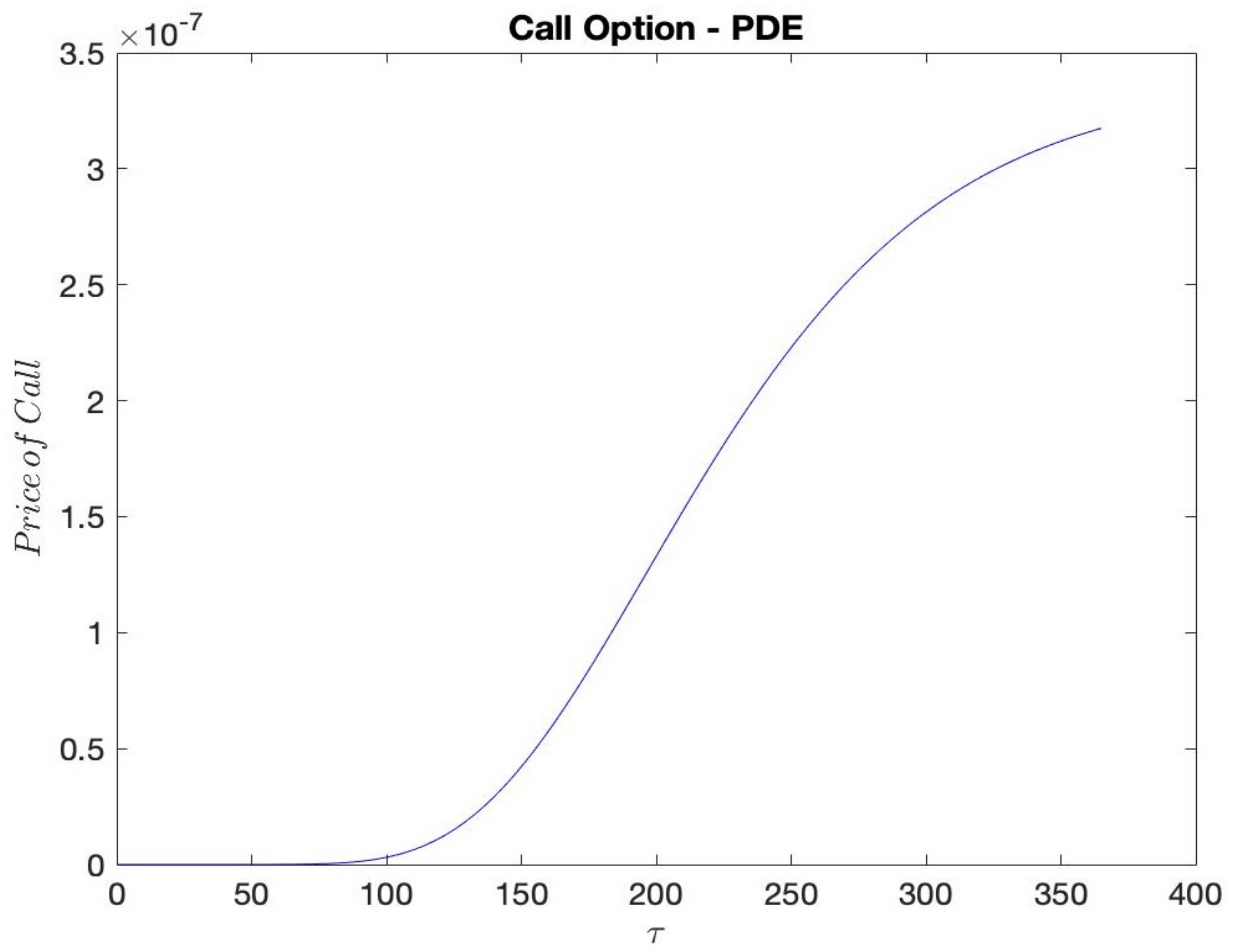
In what follows, in Figure 2, we plot the price of the call obtained by solving the fractional PDE (12).

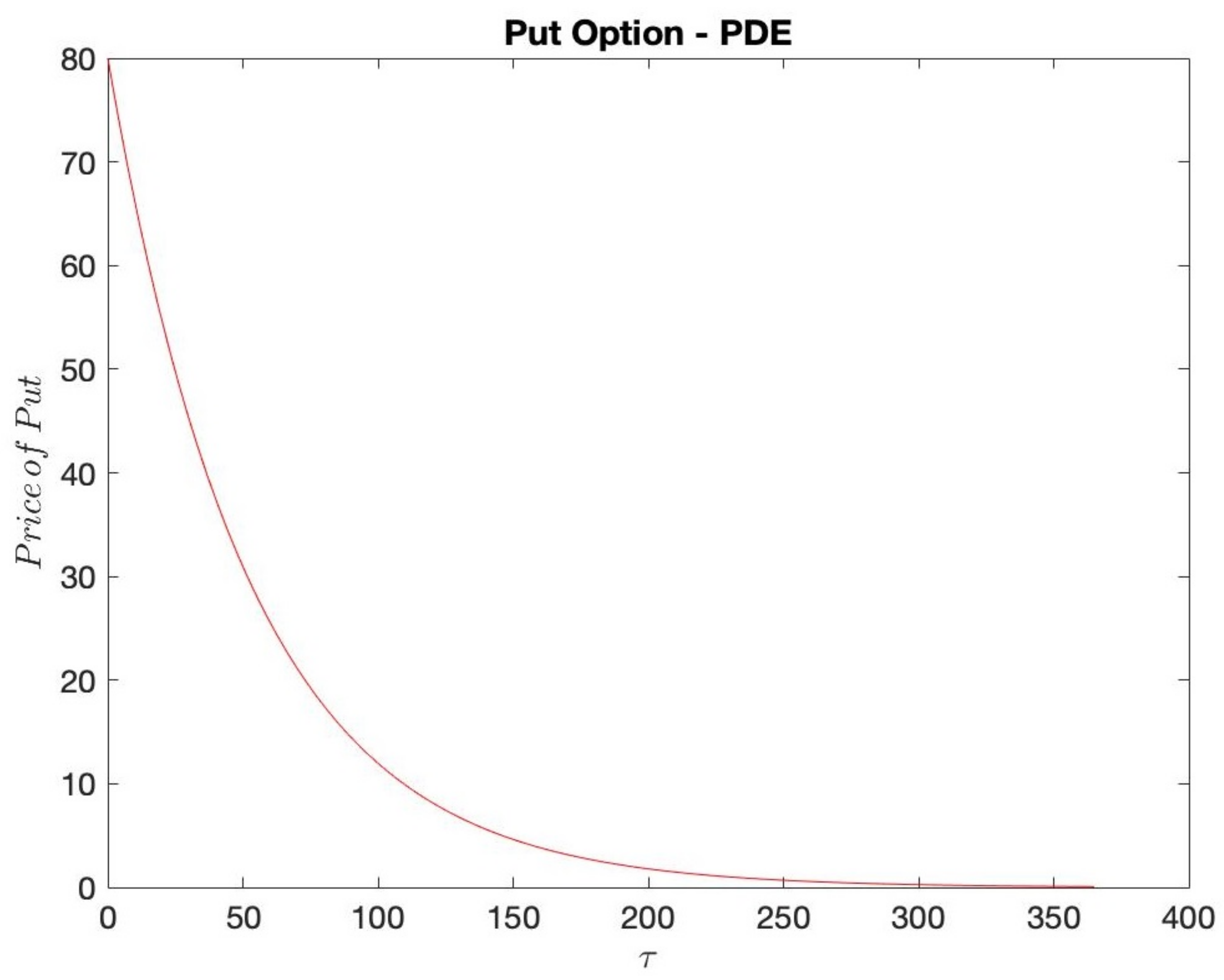
Secondly, we are interested in the calculus of the put price by using the FPDE and SDE. We use the same parameters setting in Table 1 completed by the following conditions $u(x_{max},0)=0$ and $u(x_{min},0)=K{e}^{-rT}-\frac{1}{4K}$.

In Figure 3, we plot the price of the put obtained by solving the fractional PDE (12).

Approximation of Lévy Model Greeks

In the Black and Scholes model, the derivation and analytic expressions for the Greeks for put and call prices can be done. We refer to De Olivera and Mordecki (2014) [16] for the computation of Greeks using the Fourier transform approach. However, due to the complexity of our model, we chose to use finite differences to approximate the derivatives. Then, we use the finite differences to find the Greeks (Delta “$\mathrm{\Delta }$”, Vega “$Vega$”, Gamma “$\mathrm{\Gamma }$”, Rho “$Rho$”). When this method is used to calculate Delta and Vega Greeks (first order derivative), however, the computation time is increased because the option price must be calculated more than once, multiple times in the case of the Gamma Greek (second-order derivative).

In order to approximate the first-order derivative of Greek sensitivity of the option price with respect to a parameter or to variable, we use the first-order central differences:

$${\mathrm{\Delta }}_{Levy}=\frac{\partial u(S_t,r,\sigma ,t)}{\partial S}:=\frac{u(S+dS,r,\sigma ,t)-u(S-dS,r,\sigma ,t)}{2dS},$$

(18)

and

$$Veg{a}_{Levy}=\frac{\partial u(S_t,r,\sigma ,t)}{\partial \sigma }:=\frac{u(S,r,\sigma +d\sigma ,t)-u(S-dS,r,\sigma -d\sigma ,t)}{2d\sigma },$$

(19)

and

$$Rh{o}_{Levy}=\frac{\partial u(S_t,r,\sigma ,t)}{\partial r}:=\frac{u(S,r+dr,\sigma ,t)-u(S,r-dr,\sigma ,t)}{2dr}.$$

(20)

For the second-order derivative of Greeks, such as Gamma, we use the second order central differences for a single variable:

$${\mathrm{\Gamma }}_{Levy}=\frac{{\partial }^{2}u(S_t,r,\sigma ,t)}{\partial S^2}:=\frac{u(S+dS,r,\sigma ,t)-2u(S,r,\sigma ,t)+u(S-dS,r,\sigma ,t)}{{\left(dS\right)}^2}.$$

(21)

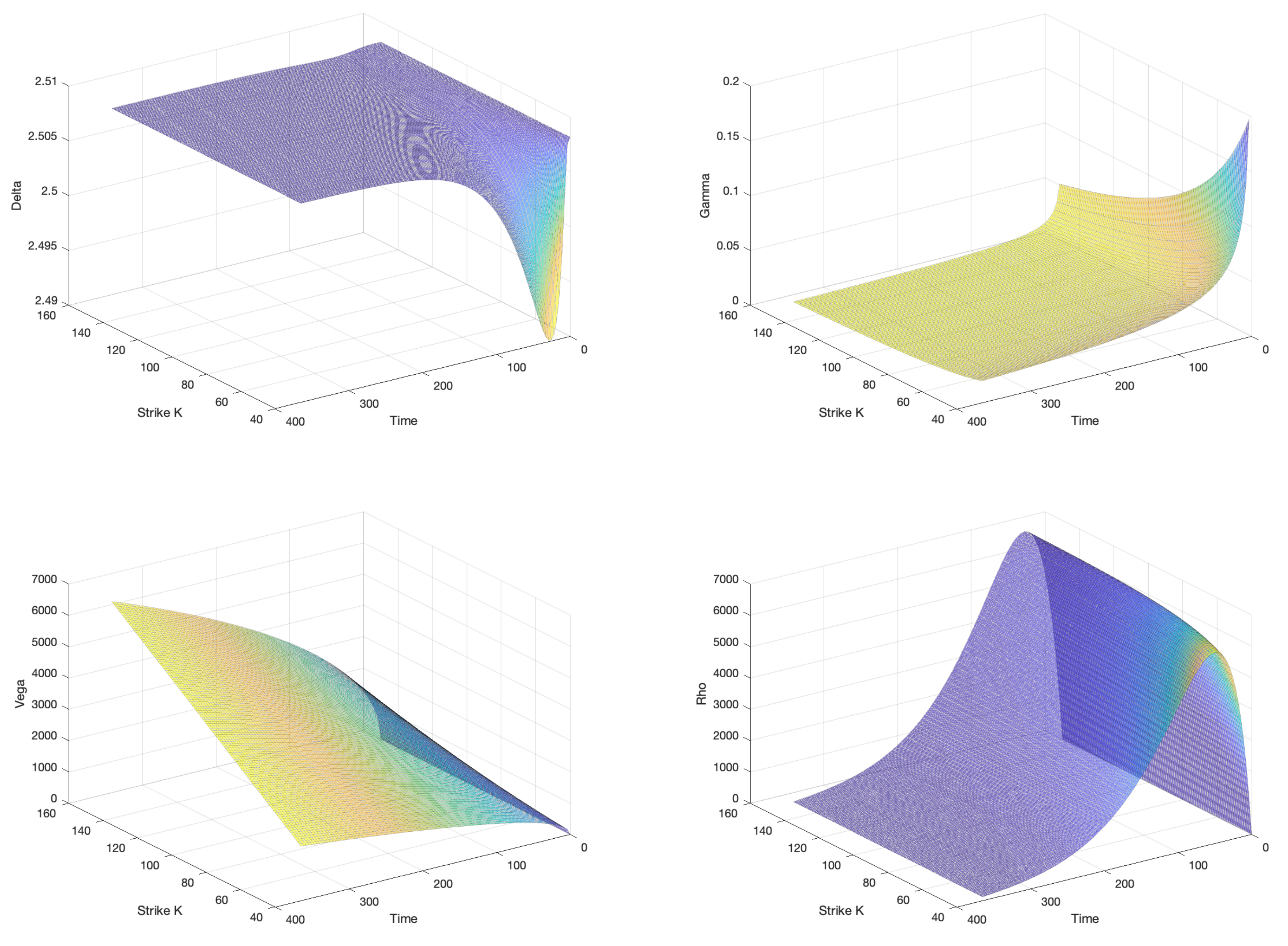
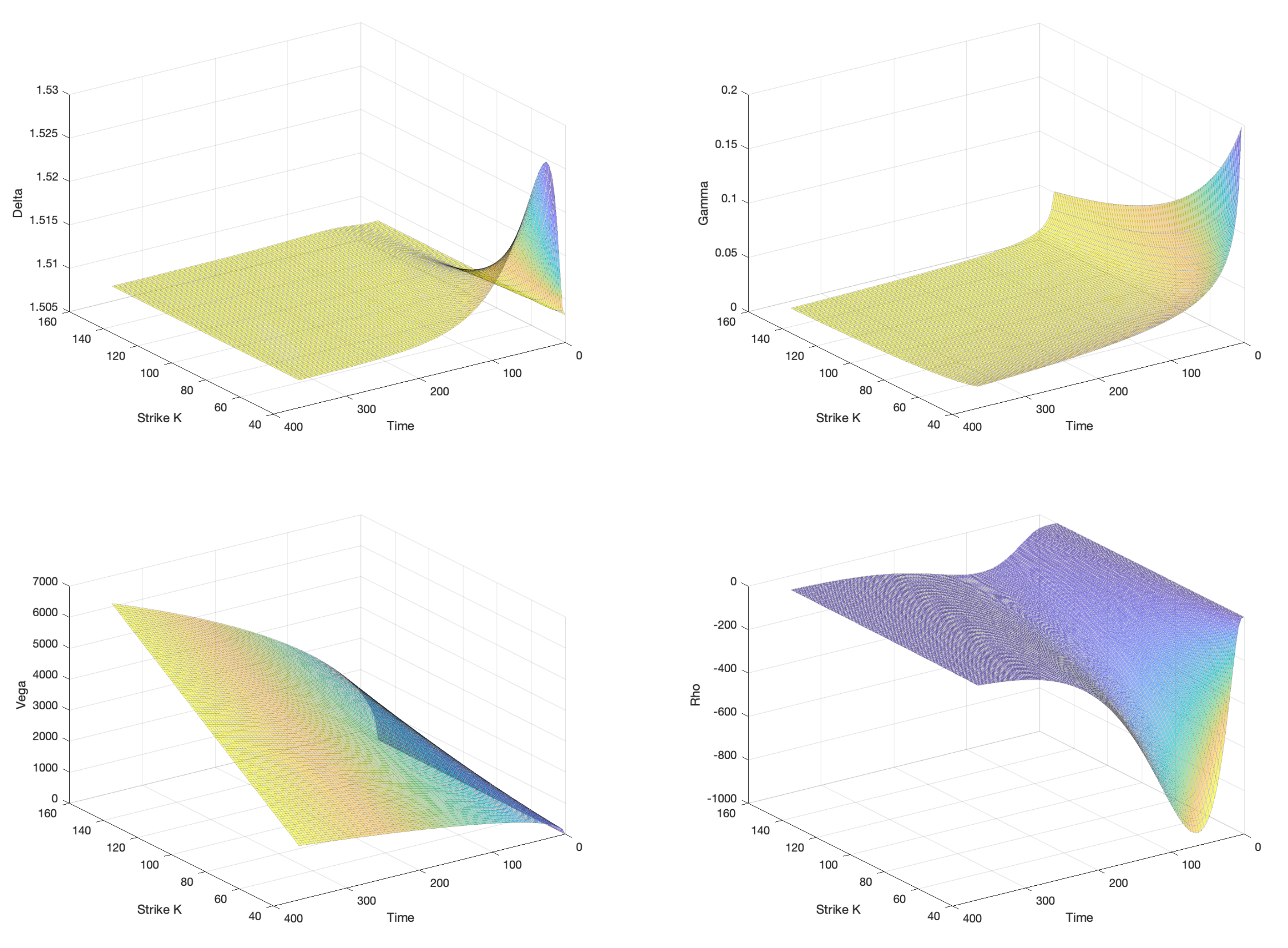
To illustrate the Greek sensitivity analysis for put and call option prices, we develop MATLAB codes. It is informative to present visual simulations of the Greeks (Delta, Vega, Gamma and Rho) in 3D. Indeed, the Figure 4 presents a plot of the Greeks for the considered Lévy model.

In Figure 5, we plot the Greeks for the put option in 3D. We show that the Delta is constant with value equal to $1.51$ for put option’s price for Lévy model, but it oscillates for Black–Scholes. We have also the same remarks for Gamma, Vega and Rho.

5. Conclusions

Through this work, the fractional diffusion equation in terms of the Lévy process is solved. We also discussed the Euler–Maruyama equation for solving the price of fractional financial derivatives of European options price.

Lévy processes have proven to be a suitable method that strikes the right balance between the properties of the mathematical approach and the value of option evolution.

Furthermore, we made a comparison between European call and put option prices based on the Lévy diffusion equation and provided numerical solutions of the fractional partial differential equation that were derived by the fractional diffusion model.

References

- Raible, S. Lévy Processes in Finance: Theory, Numerics, and Empirical Facts. Ph.D. Thesis, University of Freiburg, Freiburg im Breisgau, Germany, 2000. [Google Scholar]
- Schoutens, W. Lévy Processes in Finance, 1st ed.; Wiley Series in Probability and Statistics; John Wiley & Sons: Hoboken, NJ, USA, 2003. [Google Scholar]
- Eberlein, E. Fourier—Based Valuation Methods in Mathematical Finance. In Quantitative Energy Finance; Benth, F.E., Kholodnyi, V.A., Laurence, P., Eds.; Springer: Berlin/Heidelberg, Germany, 2014; pp. 85–114. [Google Scholar]
- Cartea, A.; del-Castillo-Negrete, D. Fractional Diffusion Models of Option Prices in Markets with Jumps; Elsevier: Amsterdam, The Netherlands, 2006. [Google Scholar]
- Abouagwa, M.; Li, J. Stochastic fractional differential Equations driven by Lévy noise under Carathéodory conditions. J. Math. Phys. 2019, 60, 022701. [Google Scholar] [CrossRef]
- Wu, P.; Yang, Z.; Wang, H.; Song, R. Time fractional stochastic differential equations driven by pure jump Lévy noise. J. Math. Anal. Appl. 2021, 504, 125–412. [Google Scholar] [CrossRef]
- Cont, R.; Voltchkova, E. Finite difference methods for option pricing in jump diffusion and exponential Lévy models. SIAM J. Numer. Anal. 2005, 43, 1596–1626. [Google Scholar] [CrossRef]
- Shokrollahi, F.; Kılıçman, A.; Ibrahim, N.A. Greeks and Partial Differential Equations for some Pricing Currency Option Models. Malays. J. Math. Sci. 2015, 9, 417–442. [Google Scholar]
- Chen, W.; Xu, X.; Zhu, S.P. Analytical pricing European-style option under the modified Black-Scholes equation with a partial-fractional derivative. Quartely Appl. Math. 2014, 72, 597–611. [Google Scholar] [CrossRef]
- Aljedhi, R.A.; Kılıçman, A. Fractional Partial Differential Equations Associated with Lévy Stable Process. Mathematics 2020, 8, 508. [Google Scholar] [CrossRef] [Green Version]
- Demirci, E.; Ozalp, N. A method for solving differential equations of fractional order. J. Comput. Appl. Math. 2012, 236, 2754–2762. [Google Scholar] [CrossRef] [Green Version]
- Shen, S.; Liu, F.; Chen, J.; Turner, I.; Anh, V. Numerical techniques for the variable order time fractional diffusion equation. Appl. Math. Comput. 2012, 218, 10861–10870. [Google Scholar] [CrossRef] [Green Version]
- Jumarie, G. Derivation and solutions of some farctional Black-Scholes equations in space and time. J. Comput. Math. Appl. 2010, 59, 1142–1164. [Google Scholar] [CrossRef] [Green Version]
- Yuste, S.B. Weighted average finite difference methods for fractional diffusion equations. J. Comput. Phys. 2006, 216, 264–274. [Google Scholar] [CrossRef] [Green Version]
- Lubich, C. Discretized Fractional Calculus. SIAM J. Math. Anal. 1986, 17, 704–719. [Google Scholar] [CrossRef]
- De Olivera, F.; Mordecki, E. Computing Greeks for Lévy Models: The Fourier Transform Approach. arXiv 2014, arXiv:1407.1343. [Google Scholar]
Figure 1.
Comparison between numerical solutions (SDE and FPDE). Upon the comparison, using the same parameters, of the left hand side of Equation (17) obtained by a FPDE approach and the right hand side of Equation (17) computed using Monte Carlo simulation, we observe that both solutions are close to each other.
Figure 2.
This figure shows the evolution of the call option price with respect to the time to maturity using the FPDE representation. In comparison with the Black–Scholes call price when the underlying is driven by the Brownian motion, the two prices have the same shape.
Figure 3.
This figure shows the evolution of the call put option price with respect to the time to maturity using the FPDE representation. In comparison with the Black–Scholes put price when the underlying is driven by the Brownian motion, the two prices have the same shape.
Figure 4.
Lévy model Greeks for the call option: By analyzing the Greeks plots, we observe that the call option’s price have much higher Delta values than out of the call option’s price of Black–Scholes model, and this value oscillates around , which ranges between and . Gamma reaches its maximum when the underlying price is a little bit smaller, exactly equal to the strike of the call option, and the chart shows that Gamma is significantly constant for the Lévy model. We display also Vega as a function of the asset price and time to maturity for a call options with strike at 80 and we highlight the fact that Vega is much higher for the call option’s price than for the call option’s price for Black–Scholes. At last, Rho reaches its maximum when the underlying price is a little smaller, not exactly equal to the strike of the call option’s price, and it is significantly higher with hyper-volatility than for the call option’s price of Black–Scholes.
Figure 5.
Lévy model Greeks for the put option: in the figures above, we plotted the Greeks for the put option in 3D. We observe that the Delta is constant with value equal to for put option’s price for Levy model, but it oscillates for Black–Scholes. We can see that the put–call parity is maintained for the Lévy model: Vega(Call) = Vega(Put) and Gamma(Call) = Gamma(Put). We have a negative Rho which ranges between and 0, and the figure displays its fluctuation with respect to the underlying asset.