
Stochastic Optimal Control Analysis of a Mathematical Model: Theory and Application to Non-Singular Kernels


1
Department of Mathematics, Sun Yat-Sen University, Guangzhou 510275, China
2
Department of Mathematics, Guizhou University, Guiyang 550025, China
*
Author to whom correspondence should be addressed.
Fractal Fract. 2022, 6(5), 279; https://0-doi-org.brum.beds.ac.uk/10.3390/fractalfract6050279
Submission received: 1 December 2021
/
Revised: 20 December 2021
/
Accepted: 27 December 2021
/
Published: 23 May 2022
(This article belongs to the Special Issue Importance of Fractional Order Derivatives in Real-World Applications: New Aspects and Understanding the Natural Phenomena)
Abstract
:Some researchers believe fractional differential operators should not have a non-singular kernel, while others strongly believe that due to the complexity of nature, fractional differential operators can have either singular or non-singular kernels. This contradiction in thoughts has led to the publication of a few papers that are against differential operators with non-singular kernels, causing some negative impacts. Thus, publishers and some Editors-in-Chief are concerned about the future of fractional calculus, which has generally brought confusion among the vibrant and innovative young researchers who desire to apply fractional calculus within their respective fields. Thus, the present work aims to develop a model based on a stochastic process that could be utilized to portray the effect of arbitrary-order derivatives. A nonlinear perturbation is used to study the proposed stochastic model with the help of white noises. The required condition(s) for the existence of an ergodic stationary distribution is obtained via Lyapunov functional theory. The finding of the study indicated that the proposed noises have a remarkable impact on the dynamics of the system. To reduce the spread of a disease, we imposed some control measures on the stochastic model, and the optimal system was achieved. The models both with and without control were coded in MATLAB, and at the conclusion of the research, numerical solutions are provided.
1. Introduction to the Problem and Model Formulation
Different types of epidemic models exist, including fractional, deterministic, stochastic, and age-structure models [1,2,3,4,5,6,7,8,9,10]. The stochastic differential equation models are more suited for mathematical modeling than the deterministic ones [1,3], because they may give a higher level of realism than their deterministic counterparts. When we run a stochastic model multiple times, we may build up a distribution of the anticipated outcomes, such as the size of infectious compartments at time t, which is more helpful than when we run a deterministic model. A deterministic model, on the other hand, will only provide a single predicted value.
Because of their extensive use, fractional integration and differentiation are rapidly growing subjects that have piqued the interest of a variety of researchers. Since then, this issue has piqued the interest of researchers from many areas [11,12,13,14,15,16,17,18,19,20,21]. The problem arose from a query posed by L’Hopital to Leibniz, which originally highlighted the issue of exponential function differentiation. At later stages, Liouville proposed a name for the derivative with a fractional index, while also cautioning that the characteristics of this new operator should not be confused with those of the integer-order derivative [11,12,13,14,15,16,22,23]. Following that, a collaboration between Liouville and Riemann produced the well-known integral of arbitrary order and, later, an arbitrary-order derivative. A derivative of a function that is continuous and a power-law function is their differential operator . The Laplace transform of this derivative produces peculiar starting circumstances that would be hard to compute otherwise [11,12,13,14,15,16].
As a result, a novel set of differential operators was required, with a few variations proposed. The Caputo–Fabrizio (CF) derivatives and the Atangana–Baleanu (AB) derivative with the Mittag–Leffler and exponential kernels are two examples. One of these operator’s peculiarities is that its kernels are non-singular [9,11,12,13,14,15,16] and that it does not satisfy several classical derivative characteristics such as the index law. These fractional derivatives do not have the same characteristics as fractional or classical derivatives with the power-law kernel because of their continuous kernels. This shows that in nature, exponential, power-law, and Mittag–Leffler functions do not all perform the same role [24,25]. There are issues in nature that follow power-law procedures; a few follow decaying procedures; many others have degradation and afterwards power-law procedures. Because the fractional derivative with a singular kernel and the fractional derivative with non-singular kernels are two different subsets of fractional calculus, both ideas may have been explored individually in a normal and constructive field. As a result, they should be addressed separately.
Nevertheless, rather than examining the characteristics of non-singular kernel fractional derivatives separately, some writers have chosen to write some ill-structured papers that combine the two sub-sets; while other research articles are based on incorrect analyses, which are the result of a lack of understanding of the entire concept. As a result, this paper will go over all of the criticisms leveled about non-singular kernels’ differential and integral operators. The following fractional calculus chaotic survival characterized by non-singular kernels was suggested in [26]:
where is the class of researchers that use the arbitrary-order operators of the differential type with non-singular kernels vulnerable to being misguided by critics (harmful) and stands for the class of those researchers that are the affectees of harmful research articles. The notion denotes those researchers that are affected and yet they have a constructive approach towards the non-singular kernel. represents those researchers that are affected and also have a bad opinion about derivatives that have a non-singular kernel. are those researchers that overcame the division of criticism, and finally, the researchers that are dead, retired, or have left the research of fractional derivatives and integrals are denoted by . The topic is extremely appealing because the notion is widely applicable; therefore, each time a new researcher joins the area, we use as the recruiting rate in this model. Naturally, some researchers working in this area may die, and as a result, they will no longer be working in the field; as a result, we will choose d as the death rate. Retirement can be explained by d as well. is interpreted as a contact coefficient, or the likelihood that a researcher will read a work concerning non-singular kernel derivatives with negative content. Similarly, the rate at which a fractional calculus researcher joins class D owing to division is represented by the parameter . is the percentage of people who are impacted by criticism, yet still believe in non-singular kernel variants. The term is the rate of recovery. Due to division, is the rate at which researchers join class , and is the rate at which persons with favorable opinions join class D. The recovery rate of the class is . The rate at which class joins class D owing to division is called . The recovery rate of class I is . The recovery rate in class D is shown by , whereas such that denotes the independent Brownian motion, and for stands for the white noise intensity.
In this work, the researchers were interested in formulating a stochastic model for the proposed social phenomenon and studying its possible control policy, besides the stability of the model. It is also of great concern to study the underlying deterministic model of the developed model, and thus, we analyzed its corresponding ODE model. The main goal of the control section of the study is to characterize the infection rate (being a control measure). This control reduces the amount of the infected population (over a given time interval), while keeping the expense of the control strategies in mind. We minimize the expected value when it comes to stochastic models. For the deterministic approach, the Hamilton–Jacobi–Bellman equation is utilized, but for the control theory of stochastic problems, the “Hamilton–Jacobi–Bellman equation” is employed. Hence, this paper reviews all issues raised against non-singular kernels’ differential and integral operators. A stochastic mathematical model depicting the survival of fractional calculus based on non-singular kernels is herein proposed and analyzed.
The rest of the article is constructed in the following fashion. In Section 2, we show the existence and uniqueness of global positive solutions of System (1) having a starting approximation. In Section 3, we give some necessary axioms for the extinction of the epidemic. In Section 4, we derive the existence of the solution of a stationary distribution by using the method of Khasminskii and making a proper Lyapunov operator. Likewise, we look into a stochastic control problem for optimality in Section 5. Some parallels were found in both the deterministic and stochastic control models. In Section 6, a few numerical simulations are presented to validate the required scheme. The main results of this paper end with the conclusion in Section 7.
2. Qualitative Analysis of the Global Non-Negative Solution
In order to investigate the dynamics of the proposed system, firstly, we are concerned about the solution being non-local and non-negative. In the following part, we make a proper “Lyapunov function” to verify the qualitative analysis of globally positive solutions of the problem (1).
Theorem 1.
For some initial approximation , a one positive root of model (1) exists on interval , and solution has one chance of occurrence, namely the solution ∀ a.s.
Proof.
For the proof of this theorem, see Theorem 5 in [26]. □
3. Extinction of the Proposed Model
We develop the conditions for model extinction in this section of the research. We include some notations and definitions below for convenience. Assume that:
Lemma 1.
Let us assume that represents a solution of Model (1) with given initial data , then:
Further, if , then:
In the following, we calculate and define the threshold parameter for the model (1):
The following is the outcome of the illness extinction.
Theorem 2.
Assume that and represent a solution to the model (1) with subsidiary conditions .
If , then:
a.s. This means that if we let (exponentially a.s.), the affectees will be removed from the community with a probability of one. Besides:
Proof.
For the proof of this theorem, see Theorem 6 in [26]. □
4. The Stationary Distribution of the Disease
Since there are no endemic equilibria in stochastic systems, as a result, the stability analysis cannot be utilized to investigate the disease’s permanence. As a result, one must focus on the uniqueness/existence hypothesis of the stationary distribution, which, in some ways, will aid in the disease’s survival. We use a well-known finding of Khasminskii [27] to illustrate this point.
Let be a Markov process and regular time and homogeneous over :
The diffusion matrix is defined as follows:
Lemma 2
([1]). The Markov processes has an ergodic stationary distribution in an open domain that is unique, bounded, and has a regular boundary, while its closure satisfies the following properties:
- 1.
- In the set U and its neighbor thereof, the eigenvalue of the diffusion matrix that has the smallest magnitude is bounded away from the origin;
- 2.
- If x is in , the average time τ in which a path starts from x reaching U is , and where K is compact. Besides, for an integrable function w.r.t measure Π, we have:
Define a parameter:
Theorem 3.
The solution of System (1) is an ergodic one, and there must exist a stationary distribution when .
Proof.
To prove Condition (2) of Lemma 2, we need to formulate a positive -function . To do so, we consider the following functions:
where and are positive constants to be determined later. By the Itô’s formula and system (1), we can get
Therefore, we have
Let
Namely,
Consequently:
In addition, we obtain:
where is constant which will be determined later. It is helpful to show that:
where . Next, we must demonstrate that has a unique minimum value
The partial derivative of with respect to , and D is as follows:
One can notice that has one and only one point of stagnation:
Furthermore, the Hessian matrix of at is:
It is clear that the Hessian matrix is positive definite. Hence, has a minimum value . Further, by using Equation (11) and utilizing the fact that is continuous, we can say that has one and only one minimum value inside . Furthermore, we have to chose another positive -function as follows:
Applying the formula of model (1), we can get and keeping in view the model, we have:
A direct consequence of the above equation is given as:
where:
To move further, we define a set in the form:
for where are very small positive real numbers to be calculated at later stages. To make the process simpler, we make a partition of the space in the form of:
□
Next, it is worth showing that on is equivalent to proving the result in the above ten sub-regions.
Case 1.
For any then by Equation (15), we obtain:
Choosing we obtain for every
Moreover, by using the inequalities in Equation (15), with the same method used for the proof of Case (1), we conclude that for all , , , , and .
Case 2.
For any then by Equation (15), we obtain:
Assuming the smallest possible value of , for every
Moreover, with a similar approach used to prove Case (2) and using Equation (15), we obtain , which can be derived for each , , , , .
In conclusion, we arrive at the final result that there must exist , such that
Hence
Assume that , and is the time at which a path starting from x approaches set D,
Integrating Relation (18) with limits zero and , assuming the concept expectation, and finally, applying Dynkin’s formula, the following result my be obtained:
As the function is positive, therefore:
By considering the results of Theorem 3, we have . Besides, from the regularity of System (1), we have that, by letting , we have almost surely.
Utilizing the well-known lemma of Fatou yields:
Clearly, where K is compact, as discussed already. Consequently, this proves Condition (2) of Lemma 2.
It also worth mentioning that the diffusion matrix of Model (1) is of the form:
Choosing we obtain:
where This means that, the criteria (1) of Lemma 2 hold. According to the above-mentioned results, one can easily conclude that Lemma 2 shows the ergodicity of Model (1), as well as its stationary distribution.
5. Stochastic Optimal Control
The use of optimal control theory techniques is becoming increasingly important, especially in the field of mathematical modeling. These techniques may be utilized to discover an effective control approach by evaluating appropriate control functions [1,3]. Control theory includes a large body of literature, and these approaches are widely used in economics, mathematical physics, and dynamical system theory [3]. The readers are advised to consult the book for the derivation of different optimality conditions and other well-known characteristics of control theory [1,3].
This section discusses the proposed model’s comparable control system. Taking into account the model’s specified hypotheses at the start of the study, as well as the control measures , , and , we create the randomized control version process that operates with it.
The control measures to be included in System (1) have the properties given below:
- The control measure shows physically the discussion about non-singular and singular kernels on social research forums such as Google scholar and Researchgate for example "https://pubpeer.com/";
- The variable describes the size of papers published/accepted, the books, etc., about non-singular and singular kernels;
- The variable stands for the qualitative aspects such as the fairness of publishers and the editorial board;
- The measure denotes a conference presenting good talks on the subject of fractional derivatives and integrals.
The study’s main goal is to figure out a proper control approach for limiting the number of infectious and vulnerable persons while increasing the number of those who survive. The equivalent stochastic control variant of System (1) assumes the following form when the control variables are taken into account:
where the conditions at time are:
To keep things simple, we use a vector of the type:
and:
here, the functions and are both time dependent. The conditions at in terms of may be written as:
The functions in Relation (21) (i.e., f and g) are vectors having components as:
Keeping in view the usefulness of the quadratic terms in the objective functional, we assumed the following functional:
where , and for and are constants and strictly greater than zero. The objective of the present work is to find a control vector that has the following property:
here, the set U denotes the control set (admissible) and is defined as:
where the terms are positive real numbers. To use the stochastic maximal criterion, we must first determine the Hamiltonian for the problem in operation:
here, stand for the inner product in the Euclidean space, whereas and describe the two independent sets of adjoint variables. Following a similar approach of maximum criteria, we have:
Here, the state represents the optimal path followed by the state variable . The condition at on the state and the final condition of the adjoint variables of Equations (24) and (25) are:
respectively. As Equation (26) shows, the optimal value of the control variable consists of adjoint variables and state of the form:
here, is computed by Equation (26). Thus, Equations (24) and (25) can be written as:
Therefore, the given “Hamiltonian” is:
The maximum principle of Pontryagin gives us the following adjoint system:
where .
Along with the condition at final time for . Similarly, the supplementary initial and final conditions are:
and:
Considering the derivative of function H with respect to the control variables gives us the characterization of the control:
Assuming the lower and upper bounds of the control variables, we have:
6. Numerical Simulations
We give some numerical simulations in order to illustrate the theoretical results obtained in this paper. We devised a technique for System (1) using the stochastic Runge–Kutta method of fourth order. The discretization transformation takes the form:
In the numerical scheme, the terms for are reserved for the Gaussian disturbances, and it has the property where is a uniform time step size. Let us choose the initial value and the parameter values from Table 1. The desired time period for simulation is considered to be .
6.1. Numerical Simulations for the Stationary Distribution and Extinction
To show the numerical illustration of Theorem 2, we chose the values in Table 1 (). Thus, the theorem suggests that if one keeps , then the disease will be eventually eliminated from the population with probability one. These facts are supported by Figure 1 as the parameter values in this case fulfill the hypothesis of the theorem. That is to say, large noises can lead the disease to extinction, which is a different phenomenon from its corresponding deterministic model (1).
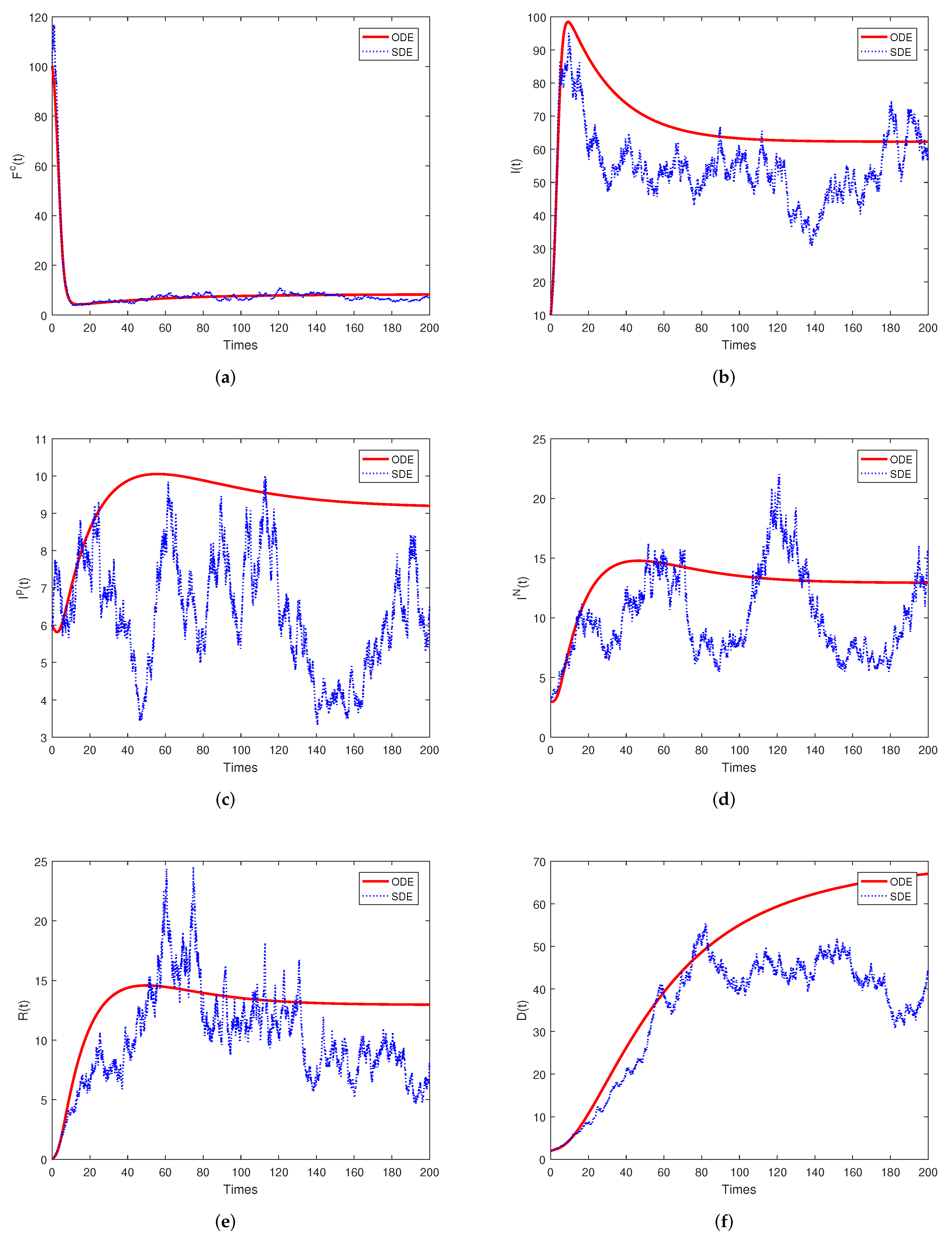
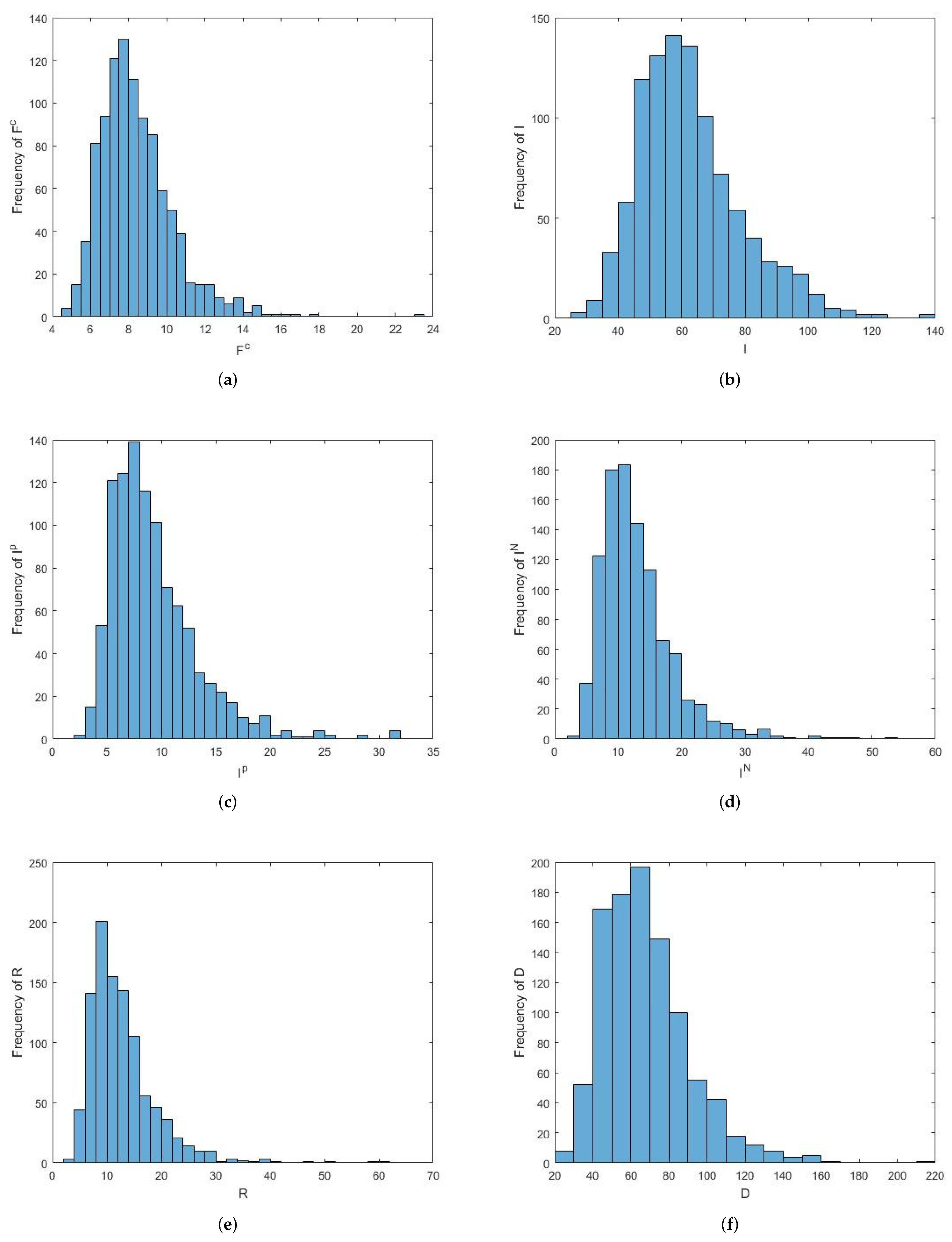
To numerically show the results suggested by Theorem 3, we take into consideration another set of parameter values in Table 1 (). This set of parameters guarantees that . When the model’s prediction is plotted (see Figure 2), it clearly shows the persistence of the infection with respect to the subject matter. By simulating the model nearly one thousand times, we calculated the average infection extinction time. It was observed that varying the noises’ intensity yielded different times of extinction. Further, it is noted that there exists an inverse relationship between the noise intensity and extinction time. We present the histograms depicting the probability of each class in Figure 3, which shows the stationary distribution as density functions, which are close to each other.
Example 1.
From the assumed values of Table 1 (), we calculated , which is less than one, and thus, by the statement of Theorem 2, the solution of the system has the following properties:
and:
These relations indicate that the dislike of fractional calculus will be eventually eliminated out of the population, and the same is validated via Figure 1.
Example 2.
By following the same procedure, we assumed the values of the parameters from Table 1 (), which satisfy the hypothesis of Theorem 3, that is greater than unity. The theorem conclusions, as well as Figure 2 and Figure 3 show that under such circumstances, the dislike of the subject matter will persist in the community.
6.2. Numerical Simulations for Stochastic Optimality
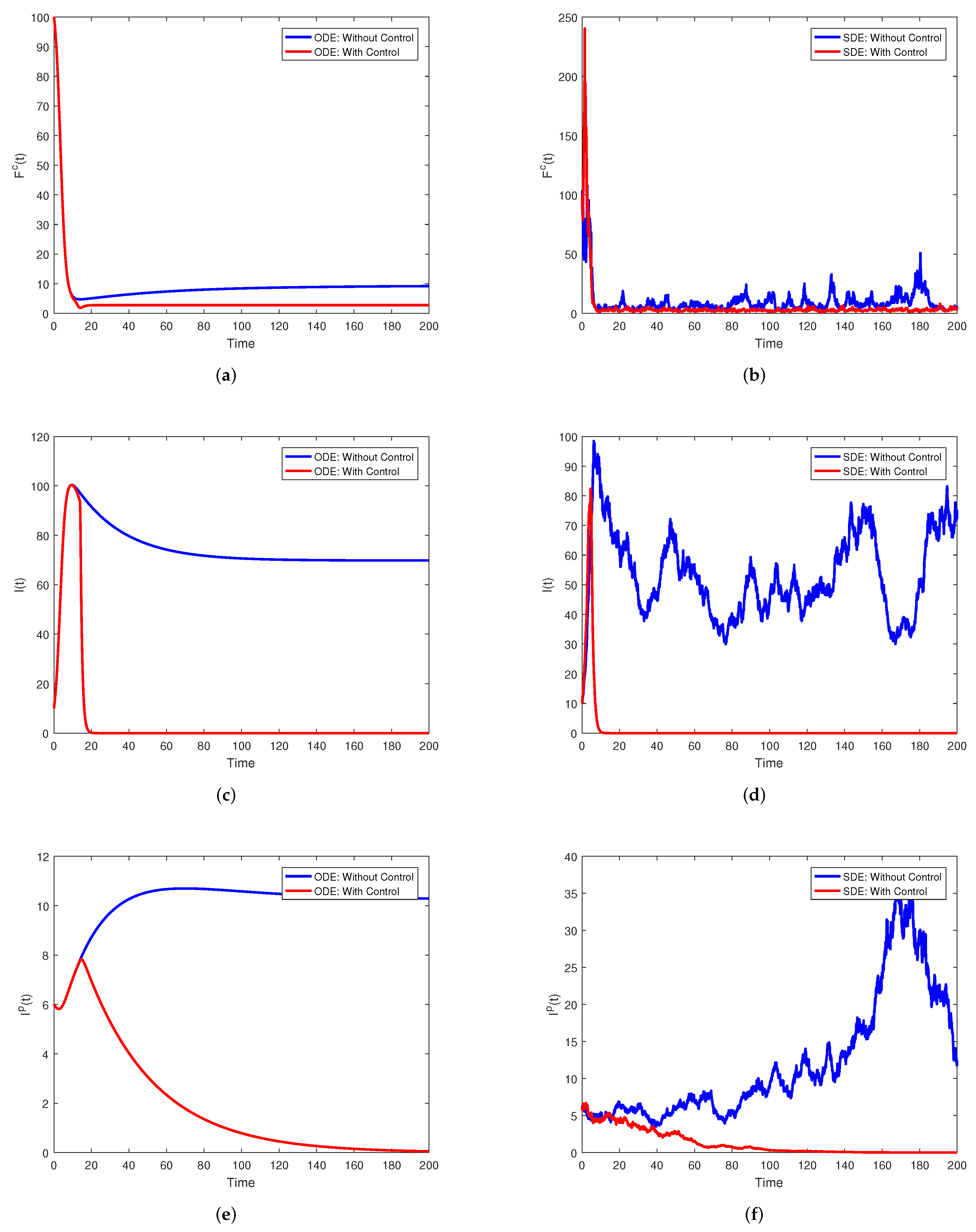
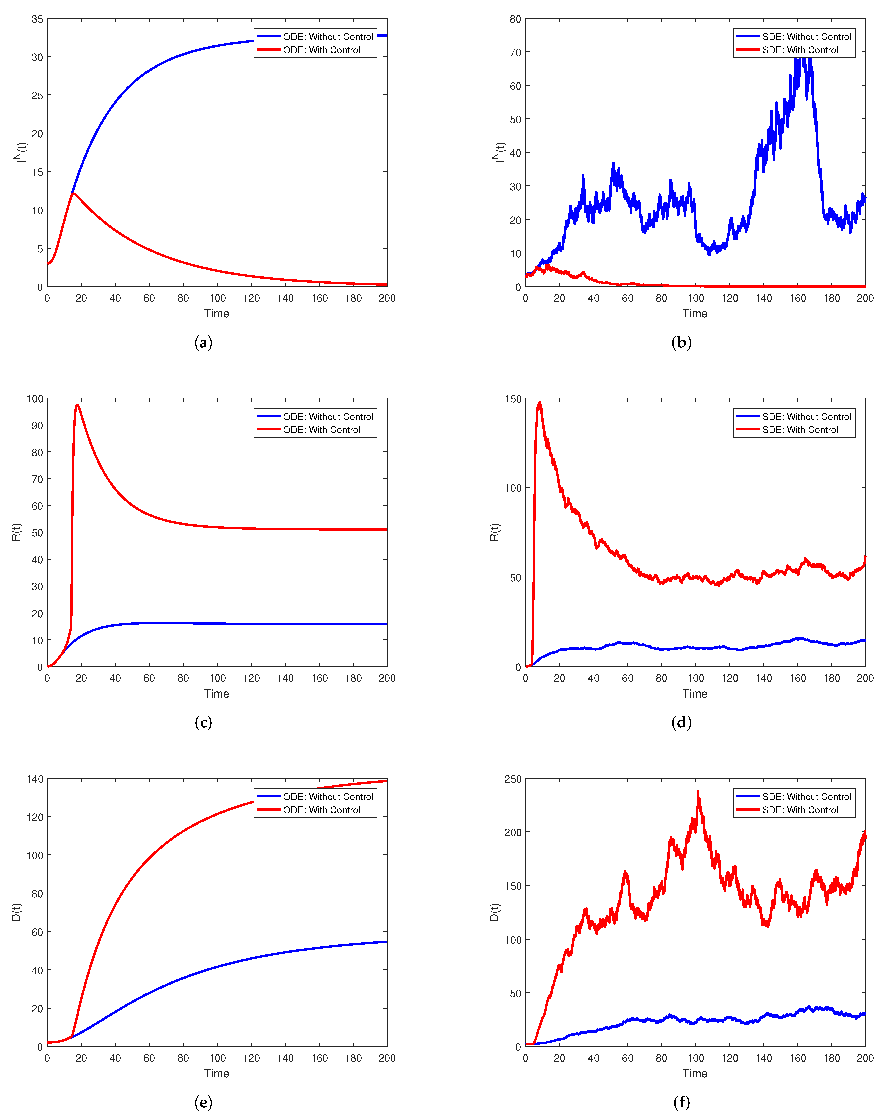
In this section, we give some numerical simulations in order to illustrate the theoretical result of the optimal control theory of the stochastic model. The method used is again the well-known RK4 method. For this simulation, the authors assumed the values of the parameters and noise intensity from Table 1 (). The figures that are of great concern are Figure 4 and Figure 5. In Figure 4a,c,e, we plot the solution curves , , and both in the presence and absence of control measures in the case of the associated deterministic system. The objective of the work is well explained by the figures. Figure 5 represents the graph of both with and without controls. Figure 5a,c,e, represents the graphs of r with and without the (optimal) control of the corresponding deterministic version of Model (1). Furthermore, Figure 4c shows the corresponding deterministic part of System (1). The effect of the control variables is clearly shown in the figures.
Besides, we used the stochastic RK4 method and simulated the proposed system (1). The numerical solution of the optimal system was obtained using the scheme that discretizes the state SDEs, the system of adjoint equations, while imposing the terminal conditions. The state system (1) was approximated with the help of RK4 techniques. After that, the same procedure was used to find a solution to the adjoint system (33) utilizing the final conditions (34). By using convex combinations of the already-obtained control measures and the formulas for the characterization of the control measures, the variables were updated. The process was repeated recursively until the desired accuracy was achieved. The figures suggest that if we impose all of the control, a drastic decrease in the I class may be observed; for instance, one can see the effect in Figure 4, Figure 5 and Figure 6.
The computed results for optimal control under the strategies are reflected in Figure 4b,d,f, and one can observe that the control strategy resulted in a decrease in the number of and the control strategy result of increasing for Model (1), while in Figure 5b,d,f, we can clearly observe the differences between the two cases with and without controls for the of Model (1). Furthermore, Figure 6 reflects the dynamics of the model’s best control variables (1). Obviously, there is a difference between these two instances.
7. Conclusions and Prediction
A divide arose as a result of the development of the fractional differential operator with non-singular kernels, which marked a significant milestone in this discipline. With the introduction of these novel integral and differential operators, potential ways for both the application and theory of fractional calculus to real-world phenomenon have opened up. Some scholars, however, anticipated differential operators with non-singular kernels to follow the characteristics of classical derivatives in the same way as fractional derivatives with singular kernels do, which is impossible because the two operators are not employed for the very same reasons. This article looked at the asymptotic behavior of a probabilistic model with nonlinear white noise disturbances. Initially, we calculated the threshold and then observed that model (1) has a stationary distribution, which is naturally ergodic. This indicates that the illness will continue to exist. This shows that stochastic disturbance can prevent negativity from spreading.
We came up with some interesting findings on the stochastic version of the optimal system control (1). The study also included suggestions for several types of control techniques. These approaches can support us in eradicating hostility in the community. To confirm the obtained analytical results, many numerical simulations were performed using the stochastic Runge–Kutta technique of fourth order. This idea might serve as a solid foundation for research into comparable illnesses, with significant implications in biologicalsciences. In addition, our suggested theory may be used to study other communicable infections including HIV, COIVD-19, and tuberculosis (TB), to name a few.
Author Contributions
Conceptualization, A.D.; Methodology, A.D.; Validation, Q.T.A.; Formal analysis, A.D., Q.T.A.; Investigation, A.D., Q.T.A.; Resources, A.D.; Data curation, Q.T.A.; Writing—original draft preparation, A.D.; writing—review and editing, A.D., Q.T.A.; Software, A.D.; Visualization, A.D., Q.T.A.; Supervision, A.D.; Project administration, A.D.; Funding acquisition, A.D. All authors have read and agreed to the published version of the manuscript.
Funding
This research was sponsored by the Fundamental Research Funds for the Central Universities, Sun Yat-sen University (Grant No. 22qntd2802).
Institutional Review Board Statement
Not applicable.
Informed Consent Statement
Not applicable.
Data Availability Statement
Data sharing not applicable to this article as no datasets were generated nor analyzed during the current study.
Acknowledgments
The authors would like to acknowledge the sponsorship from the Fundamental Research Funds for the Central Universities, Sun Yat-sen University (Grant No. 22qntd2802).
Conflicts of Interest
No conflict of interest exists regarding the publications of this paper.
References
- Din, A.; Li, Y. Stationary distribution extinction and optimal control for the stochastic hepatitis B epidemic model with partial immunity. Phys. Scr. 2021, 96, 074005. [Google Scholar] [CrossRef]
- Li, Y.X.; Rauf, A.; Naeem, M.; Binyamin, M.A.; Aslam, A. Valency-based topological properties of linear hexagonal chain and hammer-like benzenoid. Complexity 2021, 2021, 9939469. [Google Scholar] [CrossRef]
- Agarwal, R.P.; Badshah, Q.; Rahman, G.; Islam, S. Optimal control and dynamical aspects of a stochastic pine wilt disease model. J. Frankl. Inst. 2019, 356, 3991–4025. [Google Scholar] [CrossRef]
- Chen, S.-B.; Soradi-Zeid, S.; Jahanshahi, H.; Alcaraz, R.; Gómez-Aguilar, J.F.; Bekiros, S.; Chu, Y.-M. Optimal control of time-delay fractional equations via a joint application of radial basis functions and collocation method. Entropy 2020, 22, 1213. [Google Scholar] [CrossRef] [PubMed]
- Li, X.-P.; al Bayatti, H.; Din, A.; Zeb, A. A vigorous study of fractional order COVID-19 model via ABC derivatives. Results Phys. 2021, 29, 104737. [Google Scholar] [CrossRef]
- Chen, S.-B.; Rajaee, F.; Yousefpour, A.; Alcaraz, R.; Chu, Y.-M.; Gómez-Aguilar, J.F.; Bekiros, S.; Aly, A.A.; Jahanshahi, H. Antiretroviral therapy of HIV infection using a novel optimal type-2 fuzzy control strategy. Alex. Eng. J. 2021, 60, 1545–1555. [Google Scholar] [CrossRef]
- Din, A.; Li, Y. Controlling heroin addiction via age-structured modeling. Adv. Differ. Equ. 2020, 2020, 521. [Google Scholar] [CrossRef]
- Chen, S.-B.; Rashid, S.; Hammouch, Z.; Noor, M.A.; Ashraf, R.; Chu, Y. Integral inequalities via Raina’s fractional integrals operator with respect to a monotone function. Adv. Differ. Equ. 2020, 2020, 647. [Google Scholar] [CrossRef]
- Ye, W.; Khan, M.A.; Alshahrani, M.Y.; Muhammad, T. A dynamical study of SARS-COV-2: A study of third wave. Results Phys. 2021, 29, 104705. [Google Scholar]
- Din, A.; Khan, A.; Zeb, A.; Ammi, M.R.S.; Tilioua, M.; Torres, D.F.M. Hybrid Method for Simulation of a Fractional COVID-19 Model with Real Case Application. Axioms 2021, 10, 290. [Google Scholar] [CrossRef]
- Atangana, A.; Baleanu, D. New fractional derivatives with non-local and non-singular kernel, Theory and Application to Heat Transfer Model. Therm. Sci. 2016, 20, 763–769. [Google Scholar] [CrossRef] [Green Version]
- Caputo, M.; Fabrizio, M. On the notion of fractional derivative and applications to the hysteresis phenomena. Meccanica 2017, 52, 3043–3052. [Google Scholar] [CrossRef]
- Caputo, M. Linear model of dissipation whoseQ is almost frequency independent. II. Geophys. J. Int. 1967, 13, 529–539. [Google Scholar] [CrossRef]
- Leibniz, G.W. Letter from Hanover, Germany to G.F.A. L’Hospital, September 30, 1695. Math. Schr. 1849, 2, 301–302. [Google Scholar]
- Abel, N.H. Oplösning af et par opgaver ved hjelp af bestemte integraler (Solution de quelques problèmes à l’aide d’int égrales définies, Solution of a couple of problems by means of definite integrals). Mag. Nat. 1823, 2, 55–68. [Google Scholar]
- Depnath, L. A brief historical introduction to fractional calculus. Int. J. Math. Educ. Sci. Technol. 2004, 35, 487–501. [Google Scholar] [CrossRef]
- Chen, S.-B.; Beigi, A.; Yousefpour, A.; Rajaee, F.; Jahanshahi, H.; Bekiros, S.; Martínez, R.A.; Chu, Y. Recurrent neural network-based robust non-singular sliding mode control with input saturation for a non-holonomic spherical robot. IEEE Access 2020, 8, 188441–188453. [Google Scholar] [CrossRef]
- Shen, Z.-H.; Chu, Y.; Khan, M.A.; Muhammad, S.; Al-Hartomy, O.A.; Higazy, M. Mathematical modeling and optimal control of the COVID-19 dynamics. Results Phys. 2021, 31, 105028. [Google Scholar] [CrossRef]
- Saima, R.; Noor, M.A.; Ashraf, R.; Chu, Y.-M. A new approach on fractional calculus and probability density function. AIMS Math. 2020, 5, 7041–7054. [Google Scholar]
- Rashid, S.; Sultana, S.; Karaca, Y.; Khalid, A.; Chu, Y.-M. Some further extensions considering discrete proportional fractional operators. Fractals 2021, 2240026. [Google Scholar] [CrossRef]
- Balzotti, C.; D’Ovidio, M.; Loreti, P. Fractional SIS epidemic models. Fractal Fract. 2020, 4, 44. [Google Scholar] [CrossRef]
- Almeida, R.; Qureshi, S. A fractional measles model having monotonic real statistical data for constant transmission rate of the disease. Fractal Fract. 2019, 3, 53. [Google Scholar] [CrossRef] [Green Version]
- Wang, Y.; Chen, Y. Dynamic analysis of the viscoelastic pipeline conveying fluid with an improved variable fractional order model based on shifted Legendre polynomials. Fractal Fract. 2019, 3, 52. [Google Scholar] [CrossRef] [Green Version]
- Tateishi, A.A.; Ribeiro, H.V.; Lenzi, E.K. The role of fractional time-derivative operators on anomalous diffusion. Front. Phys. 2017, 5, 52. [Google Scholar] [CrossRef] [Green Version]
- Hristov, J. Steady-state heat conduction in a medium with spatial non-singular fading memory: Derivation of Caputo-Fabrizio space-fractional derivative from Cattaneo concept with Jeffreys Kernel and analytical solutions. Therm. Sci. 2017, 21, 827–839. [Google Scholar] [CrossRef] [Green Version]
- Atangana, A. Mathematical model of survival of fractional calculus, critics and their impact: How singular is our world? Results Phys. 2021, 31, 105208. [Google Scholar] [CrossRef]
- Khasminskii, R. Stochastic Stability of Differential Equations; Springer Science & Business Media: Berlin/Heidelberg, Germany, 2011; Volume 66. [Google Scholar]
Figure 1.
Simulations of for the stochastic model (1) with its corresponding deterministic version. (a) : researchers using fractional differential operators with non-singular kernels. (b) : researchers that have been affected by the harmful papers. (c) : researchers that have been affected, but still have positive opinions about non-singular kernel derivatives. (d) : researchers that have been affected and have negative opinions about non-singular kernel derivatives. (e) : researchers that have overcome divisive criticism. (f) : researchers that die, or retire.

Figure 2.
Simulations of for the stochastic model (1) with its corresponding deterministic version. (a) : researchers using fractional differential operators with non-singular kernels. (b) : researchers that have been affected by the harmful papers. (c) : researchers that have been affected, but still have positive opinions about non-singular kernel derivatives. (d) : researchers that have been affected and have negative opinions about non-singular kernel derivatives. (e) : researchers that have overcome divisive criticism. (f) : researchers that die, or retire.

Figure 3.
The probability distribution histogram of for the stochastic model (1). (a) : researchers using fractional differential operators with non-singular kernels. (b) : researchers that have been affected by the harmful papers. (c) : researchers that have been affected, but still have positive opinions about non-singular kernel derivatives. (d) : researchers that have been affected and have negative opinions about non-singular kernel derivatives. (e) : researchers that have overcome divisive criticism. (f) : researchers that die, or retire.

Figure 4.
Simulations of for the stochastic model (1) with its corresponding deterministic version, both with and without control. (a) in the case of the deterministic model both with and without control. (b) in the case of the stochastic model both with and without control. (c) in the case of the deterministic model both with and without control. (d) in the case of the stochastic model both with and without control. (e) in the case of the deterministic model both with and without control. (f) in the case of the stochastic model both with and without control.

Figure 5.
Simulations of for the stochastic model (1) with its corresponding deterministic version, both with and without controls. (a) in the case of the deterministic model both with and without control. (b) in the case of the stochastic model both with and without control. (c) in the case of the deterministic model both with and without control. (d) in the case of the stochastic model both with and without control. (e) in the case of the stochastic model both with and without control. (f) in the case of the stochastic model both with and without control.

Figure 6.
Simulations of for the stochastic model (1) with its corresponding deterministic version. (a) Trajectories of the optimal control of the deterministic system with and without control. (b) Trajectories of the optimal control of the stochastic system with and without control.
Figure 6.
Simulations of for the stochastic model (1) with its corresponding deterministic version. (a) Trajectories of the optimal control of the deterministic system with and without control. (b) Trajectories of the optimal control of the stochastic system with and without control.


Table 1.
Values of the parameters for simulating Model (1).
Table 1.
Values of the parameters for simulating Model (1).
| Parameters | Unite | |||
|---|---|---|---|---|
| Per week | 0.05 | 2.5 | 2.8 | |
| d | Per week | 1/170.365 | 1/70.365 | 1/70.365 |
| Per week | 0.08 | 0.9 | 0.8 | |
| Per week | 0.01 | 0.08 | 0.8 | |
| Per week | 0.04 | 0.07 | 0.5 | |
| Per week | 0.004 | 0.07 | 0.004 | |
| Per week | 0.02 | 0.04 | 0.04 | |
| Per week | 0.004 | 0.004 | 0.005 | |
| Per week | 0.01 | 0.03 | 0.03 | |
| Per week | 0.03 | 0.1 | 0.1 | |
| v | Per week | 0.01 | 0.01 | 0.01 |
| Per week | 0.02 | 0.001 | 0.01 | |
| Noise intensity | 0.4 | 0.4 | 2 | |
| Noise intensity | 0.3 | 0.2 | 0.3 | |
| Noise intensity | 0.4 | 0.5 | 0.4 | |
| Noise intensity | 0.5 | 0.5 | 0.5 | |
| Noise intensity | 0.6 | 0.6 | 0.1 | |
| Noise intensity | 0.2 | 0.1 | 0.2 | |
| Initial value | 100 | 60 | 430 | |
| Initial value | 10 | 50 | 10 | |
| Initial value | 06 | 40 | 30 | |
| Initial value | 03 | 35 | 20 | |
| Initial value | 00 | 15 | 10 | |
| Initial value | 02 | 15 | 10 |
Publisher’s Note: MDPI stays neutral with regard to jurisdictional claims in published maps and institutional affiliations. |
© 2022 by the authors. Licensee MDPI, Basel, Switzerland. This article is an open access article distributed under the terms and conditions of the Creative Commons Attribution (CC BY) license (https://creativecommons.org/licenses/by/4.0/).
Share and Cite
MDPI and ACS Style
Din, A.; Ain, Q.T. Stochastic Optimal Control Analysis of a Mathematical Model: Theory and Application to Non-Singular Kernels. Fractal Fract. 2022, 6, 279. https://0-doi-org.brum.beds.ac.uk/10.3390/fractalfract6050279
AMA Style
Din A, Ain QT. Stochastic Optimal Control Analysis of a Mathematical Model: Theory and Application to Non-Singular Kernels. Fractal and Fractional. 2022; 6(5):279. https://0-doi-org.brum.beds.ac.uk/10.3390/fractalfract6050279
Chicago/Turabian StyleDin, Anwarud, and Qura Tul Ain. 2022. "Stochastic Optimal Control Analysis of a Mathematical Model: Theory and Application to Non-Singular Kernels" Fractal and Fractional 6, no. 5: 279. https://0-doi-org.brum.beds.ac.uk/10.3390/fractalfract6050279