
Oscillators Based on Fractional-Order Memory Elements


Faculty of BERG, Technical University of Kosice, Nemcovej 3, 042 00 Kosice, Slovakia
Fractal Fract. 2022, 6(6), 283; https://0-doi-org.brum.beds.ac.uk/10.3390/fractalfract6060283
Submission received: 22 April 2022
/
Revised: 16 May 2022
/
Accepted: 22 May 2022
/
Published: 24 May 2022
(This article belongs to the Special Issue Fractional-Order Circuit Theory and Applications)
Abstract
:This paper deals with the new oscillator structures that contain new elements, so-called memory elements, known as memristor, meminductor, and memcapacitor. Such circuits can exhibit oscillations as well as chaotic behavior. New mathematical models of fractional-order elements and whole oscillator circuits are proposed as well. An illustrative example to demonstrate the oscillations and the chaotic behavior through the numerical solution of the fractional-order circuit model is provided.
1. Introduction
Although classical electrical elements such as a resistor, capacitor, and inductor have been known for a long time, memristors, memcapacitors, and meminductors are relatively new nonlinear elements with memory [1]. As a novel memory device, the memristor was postulated by Leon Chua in 1971 [2] and manufactured for the first time in 2008 by HP Labs [3]. Until this time, an investigation of the memristor concept was very limited due to the lack of a solid-state implementation of this postulated device.
The memcapacitor and meminductor are also members of a huge family of new circuit elements postulated by Leon Chua in 1978 [4]. The idea of Chua extended the concept of memory elements in an electrical circuit to capacitive and inductive systems, respectively. The memcapacitor and the meminductor were formally defined and described in 2009 [5]. Some elements of the electronic circuit, namely the memcapacitor and the meminductor, require not only the well-known four state variables but also the time integrals of the electric charge and flux [6]. These new state variables, due to integration, lead us to so-called “memory” devices, which are a particular class of higher-order elements (devices) and belong to a broad group of memory systems [4]. They are passive memory devices that can store information without a power supply. Currently, the applications of these memory devices in nonlinear circuits have gained a great deal of attention, and their potential value has attracted many researchers. However, the absence of semiconductor implementation of memcapacitors and meminductors prevents the use of unique functions of these devices in practical implementation. Their properties were so far investigated mainly via mathematical models, equivalent circuits, or emulators [7,8,9,10]. Such investigation is not accurate because it analyzes just their approximation, not fundamental elements.
There are also a considerable number of electrical circuits where non-integer order (or fractional) calculus can be used (see, for example, [11,12,13,14], etc.), with classical electrical circuit theory being limited to variables u (voltage), i (current), q (charge), and (flux), which are used to describe all four essential components (resistor, capacitor, inductor, and memristor). Models of the non-integer order can also describe the type noted above of memristive systems [15,16,17,18,19,20,21]. In addition, in practice, there is no ideal electrical element, and almost all electrical elements lie between two ideal ones, for example, a fractor (resistor/capacitor) or a fractductor (resistor/inductor) [12,22,23]. Here, we consider it also for the real memristive elements. That means that all real memristive elements should lie in between two ideals, similar to the classical electrical elements noted above. We used a mathematical model of supposed new fractional-order memory elements in the specific oscillator circuit. According to the author’s best knowledge, such an oscillator structure described in this article was used for the first time.
In this article, a new oscillator based on memory devices is studied. The rest of the manuscript is structured as follows: In Section 2 a definition of the fractional calculus and method for the numerical solution of the initial value problem is described. Section 3 presents the fractional-order elements models. In Section 4 the new fractional-order models of the oscillator circuits are proposed. In Section 5 some ideas for further research are discussed. Section 6 concludes this article with some additional comments.
2. Preliminaries
2.1. Definition of Fractional-Order Operator
Fractional calculus has been known since regular calculus, probably with the first evidence dated 30 September 1695, in letter correspondence between Gottfried W. Leibniz and Guillaume de l’Hospital. They mentioned a half order derivative for the first time. The fractional calculus is a generalization of differentiation and integration to common non-integer -order, , operator , where a and t of interval are the bounds of the join operation (fractional-order integrals for and derivatives for ).
There are many different definitions for the fractional-order operator , but in this paper, we will limit ourselves only to two fundamentals: Caputo’s definition (CD), and Grünwald–Letnikov’s definition (GLD).
The CD can be written as [24]:
where denotes Euler gamma function. The CD can be used for electrical circuits where non-integer order derivatives are used in the fractional (non-integer) order model of electrical circuit elements. The main benefit is that the initial conditions for fractional differential equations with Caputo derivatives are the same as for ordinary differential equations, i.e., , .
2.2. Numerical Solution of Fractional Differential Equation
Based on the fact that both definitions, CD, and GLD, are equivalent for a wide class of the functions, for numerical calculation of the fractional-order derivative, we can use the relation (3) derived from the GLD (2). The relation for the numerical approximation of the th derivative at the points has the following form [24]:
where is the “memory length”, , is the time step of calculation (definition (3) is valid only as tends towards 0 and that the accuracy of the simulation depends on the value of ), and are the binomial coefficients. For their calculation we may use the following expression:
Thus, general numerical solution of the fractional differential equation
can be expressed as follows [22]:
For the memory term expressed by the sum in (5), a “short memory” principle for various memory lengths of can be used. An evaluation of the effect of the memory length and convergence relation of the error between short and long memory was described in [24]. However, this article uses a whole (long) memory to preserve calculation accuracy.
3. Fractional-Order Memristive Elements
Many authors have so far studied the real capacitor and the real inductor, and the experimental evidence of their non-integer order of models has undoubtedly been confirmed [13,26]. The real memristor, memcapacitor, and meminductor have not yet been experimentally studied, only using their simulation models or emulators [10,27,28]. It is because they do not exist as a single component except, for the memristor element constructed in the HP Lab in 2008. However, there are many electrical circuits where memristors, memcapacitors, and meminductors have been used on the theoretical level [29,30,31,32].
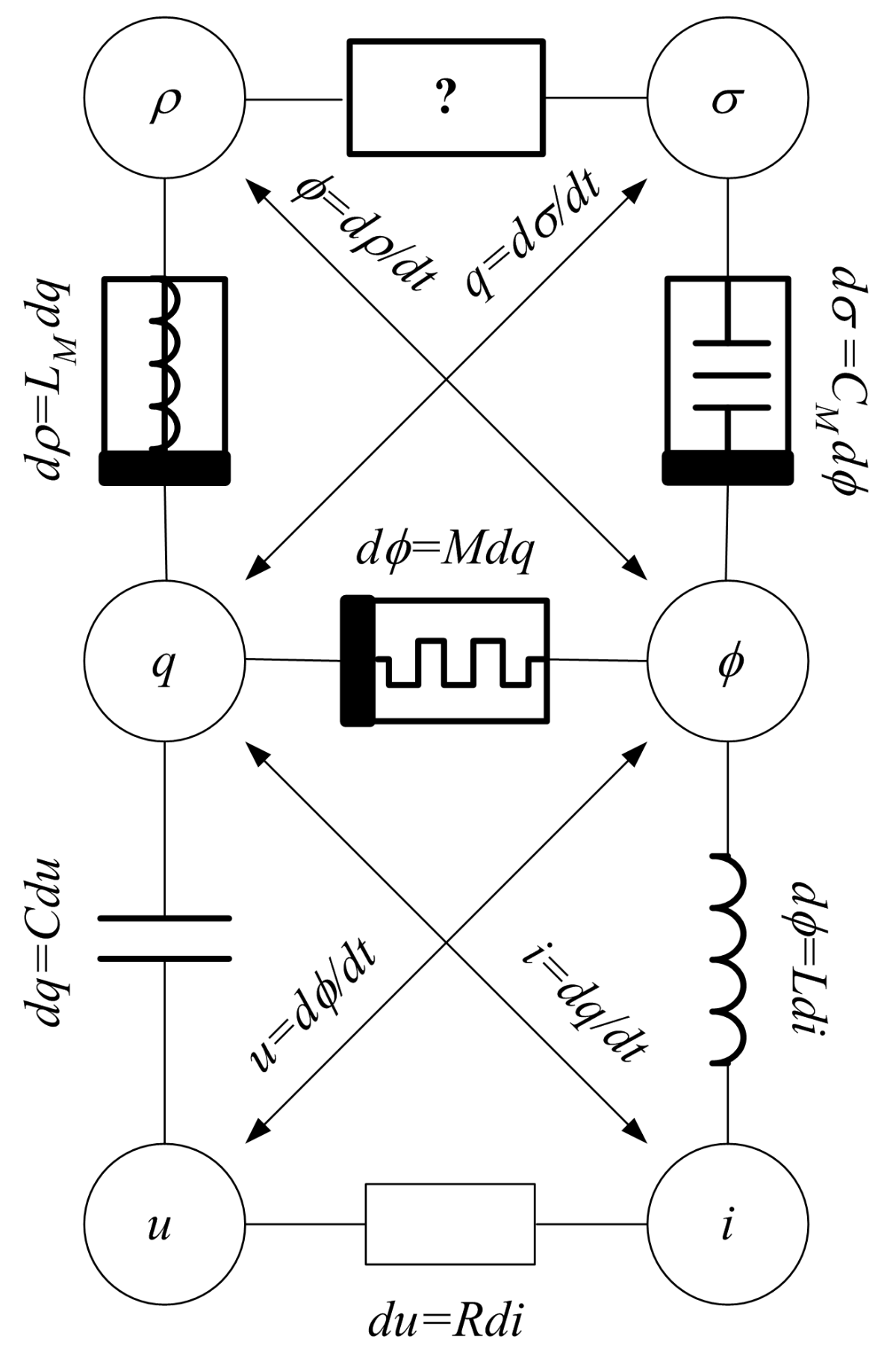
Using the relations described in [6] for memcapacitor and meminductor and the well-known connections between the four essential components (resistor, capacitor, inductor, memristor), we can obtain the next floor using the square symmetry shown in Figure 1.
However, as we can observe in Figure 1, there could be some additional electrical element that has not been discovered yet.
3.1. Memristor
The memristor used in this article is a flux-controlled memristor that is characterized by the relation
where is a memductance of the memristor. Here, we consider the following model:
where and are real constants. The memductance function W that is obtained from the function is [30]:
Moreover, for such a memristor, a monotone-increasing piecewise-linear characteristic was assumed in [34] and used in [35].
3.2. Memcapacitor
An ideal charge-controlled memcapacitor is defined as [5,31]:
where is the charge on the memcapacitor and is the corresponding voltage across memcapacitor at time t, is the time-domain integral of electric charge q passing through the memcapacitor, is the flux that goes through the memcapacitor, and is the inverse memcapacitance, which depends on the state of the device. In this paper, a charge-controlled memcapacitor is formulated in accordance with its definition [31]:
where and are constants, and their units are and , respectively.
Following a linear capacitor model proposed by Westerlund and Ekstam in 1994, for a general input voltage , applied at , the current is [26]:
where C is the capacitance of the capacitor with unit [F/s]. It is related to the kind of dielectric. Another constant (order), , is related to the losses of the capacitor. We may predict a fractional-order model of the real memcapacitor as well [15,17].
3.3. Meminductor
Similar to the definition of a memcapacitor, the ideal flux-controlled meminductor is given as [5,31]:
where and denote the flux and current go through a meminductor at time t, is the time-domain integral of electric flux passing through the meminductor, is the charge that goes through the meminductor, which is a function of , and is the inverse meminductance, which depends on their inner variables. By providing a concrete expression of , the flux-controlled mathematic model is shown as follows [31]:
where and are constants, and their units are and , respectively.
For a linear inductor model suggested in [13,36], the voltage is
where L is the inductance of the inductor with unit [H/s]. It is related to the kind of coil core material and depends on the geometry of inductor. Another constant (order), , is related to the proximity effect of the inductor. Similarly, we may predict a fractional-order model of the real meminductor as well [15].
4. Models of the Fractional-Order Chaotic Systems
4.1. Memcapacitor–Meminductor Oscillator
Let us start with the oscillator structure consisting of two memory elements, namely meminductor and memcapacitor, which was designed in [31].
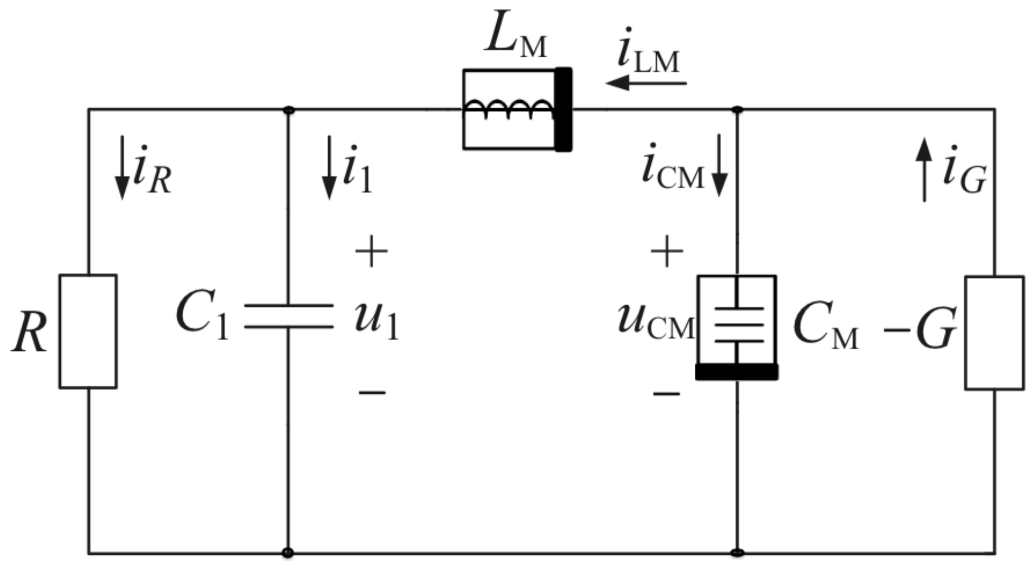
Based on the aforementioned charge-controlled memcapacitor and flux-controlled meminductor, a novel chaotic circuit is depicted in Figure 2. The suggested oscillator consists of a meminductor (), a memcapacitor (), a capacitor (), a linear resistor (R), and a negative resistor (). This circuit is also supplied by energy for maintaining the oscillating state.
According to Kirchhoff’s laws for two current nodes and one voltage loop, the following set of differential equations is obtained [31]:
Substituting Equations (10) and (13) into the above Equation (15), then adding the two well-known relations: and to them ( is the integral of flux passing through the meminductor, is the integral of charge passing through the memcapacitor), we obtain the differential equations [31]:
For additional dynamical analysis, by setting and scale transformations , , , , , the dynamical system (16) converts into dimensionless form as follows [31]:
where its parameters are: , , , , , , , , , , and .
The nonlinear dynamical system (17), depicted in Figure 2, will exhibit chaotic attractor for the following parameters [31]: , , , , , , , , , and the initial values setting: , , , , .
Taking into account the consideration described in the previous section, the fractional-order models of the elements (capacitor, memcapacitor, and meminductor) used in the chaotic oscillator shown in Figure 2 could be applied to Kirchhoff laws. Then, instead of the system (17), we obtain the following set of fractional differential equations:
where , , , , and are the real orders of aforementioned elements used in the chaotic oscillator displayed in Figure 2.
For simulation purposes, a numerical solution of the fractional differential Equation (18) obtained using the relationships (3)–(5), was proposed [38]:
where is the simulation time, is the calculation time step, , for , and initial conditions are (, , , , ). The binomial coefficients , , , , and are calculated according to relation (4), respectively.
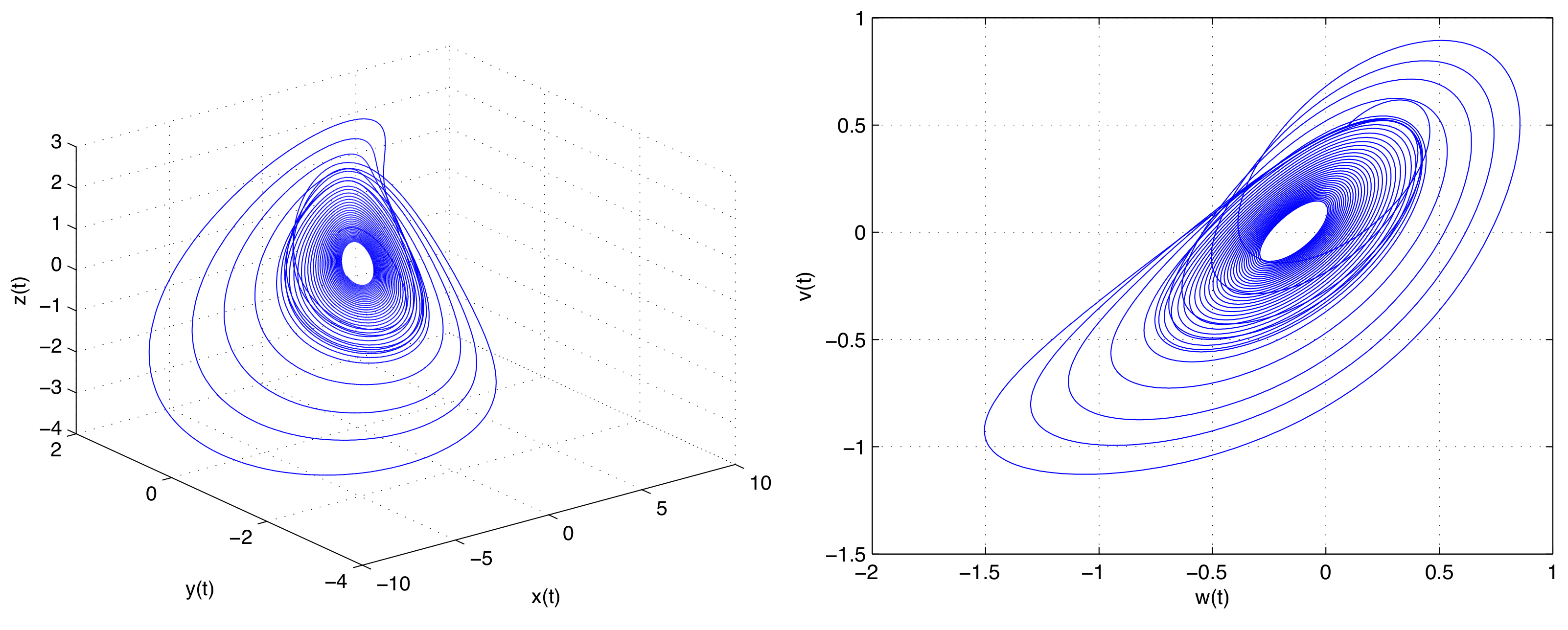
Figure 3 depicts the simulation results of the system (18) using numerical solution (19) for the parameters: , , , , , , , , , orders (real capacitor ), (ideal memcapacitor and ideal meminductor ), initial conditions , , , , , step , and simulation time 500 s. The Lyapunov exponents of this system with the above parameters, computed according to the algorithm described in [39], have the following values: , which confirm the system is chaotic because at least one exponent is positive.
4.2. Memristor–Memcapacitor–Meminductor Oscillator
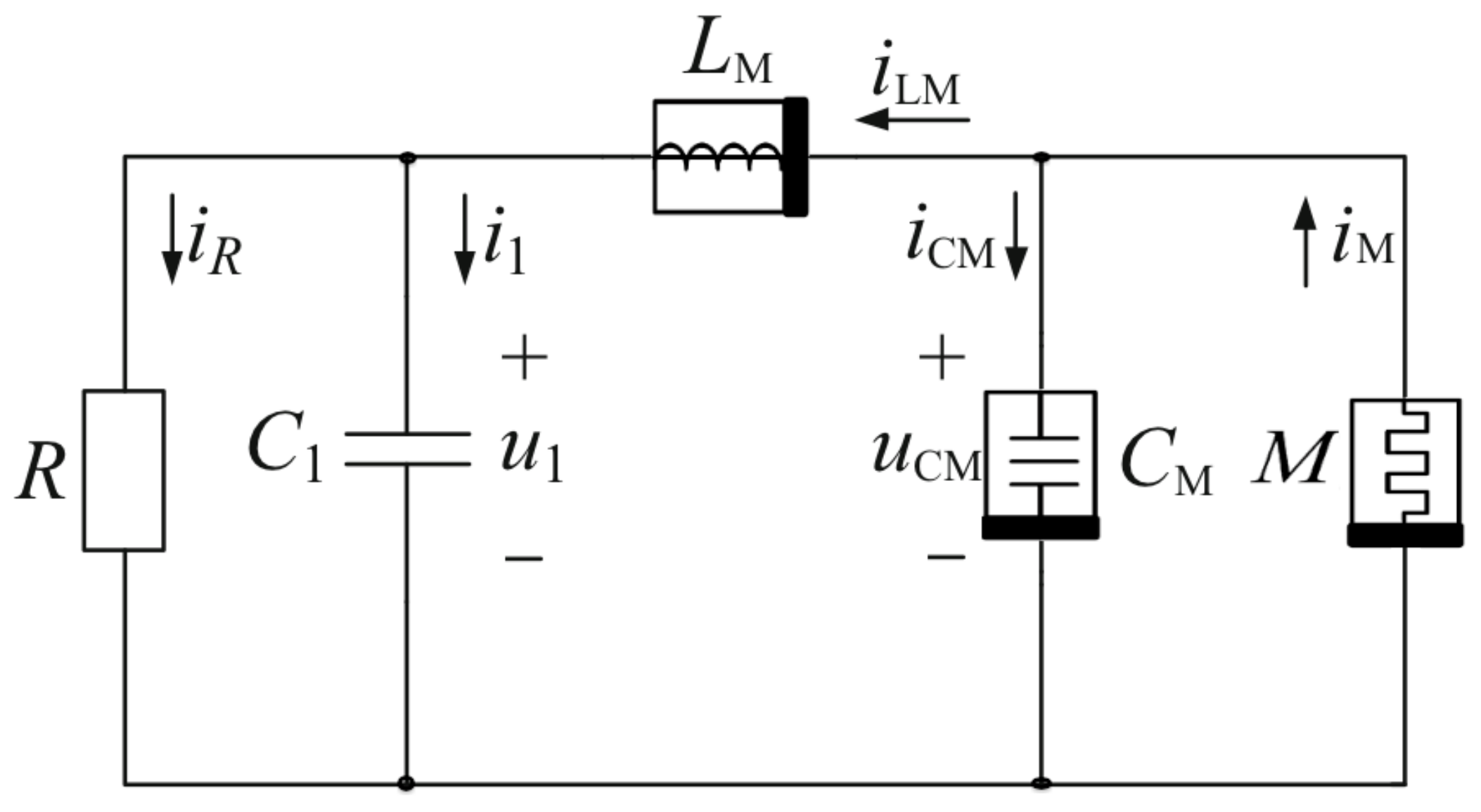
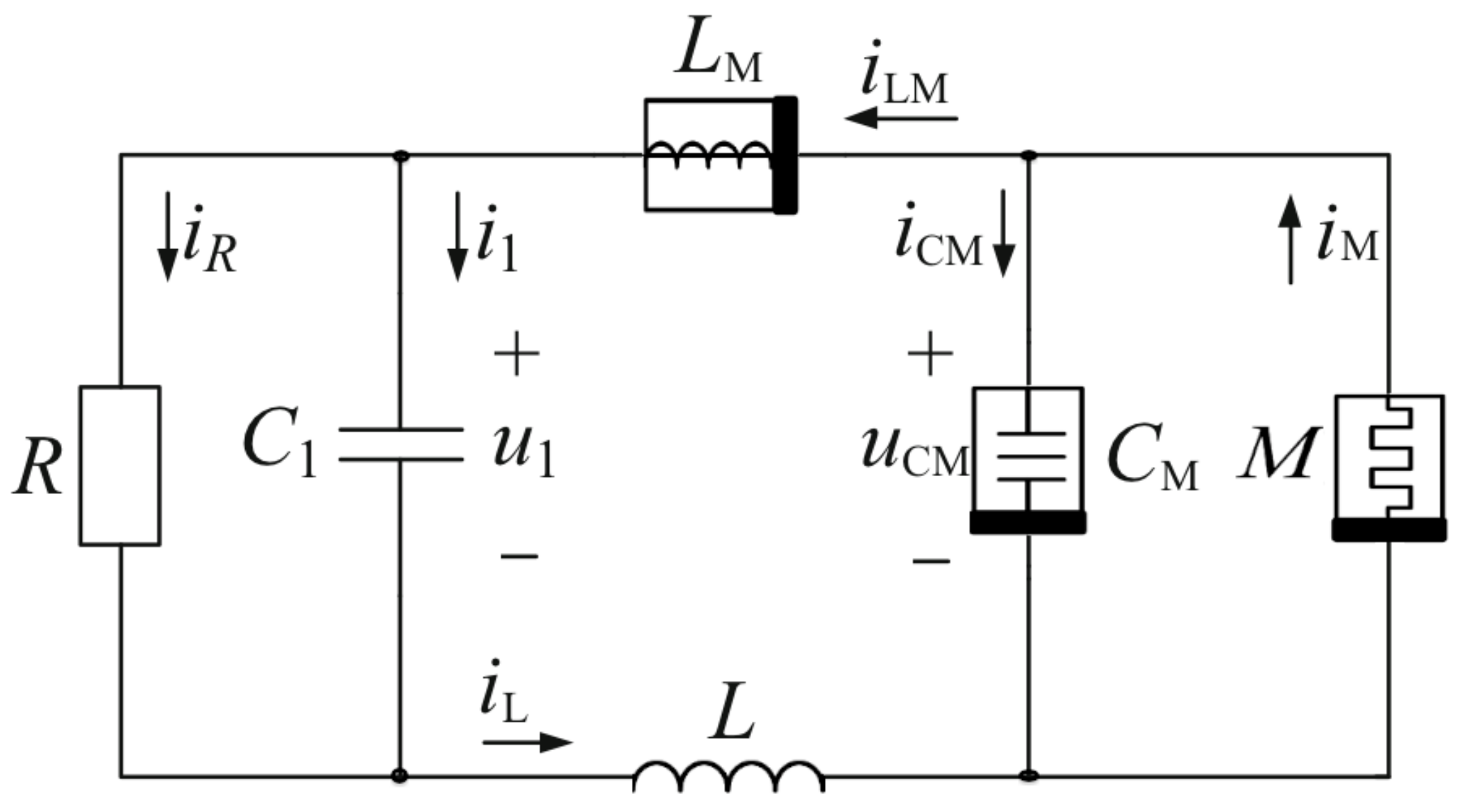
Following the oscillator based on the charge-controlled memcapacitor and the flux-controlled meminductor, which was described in the previous subsection, a novel chaotic circuit containing the flux-controlled memristor (8) instead of the negative resistor was suggested, depicted in Figure 4. The proposed oscillator consists of a meminductor (), a memristor (M), a memcapacitor (), a linear resistor (R), and a capacitor (). As in the previous case, this novel circuit is also supplied by energy to maintain the oscillating state.
According to Kirchhoff’s laws for two current nodes and one voltage loop, the following set of differential equations can be obtained:
Substituting Equations (6), (8), (10) and (13) into the above Equation (20), the same as in the previous case, adding the two well-known relations: and to them ( is the integral of flux passing through the meminductor, is the integral of charge passing through the memcapacitor), we get the following set of equations:
By setting the same state variables transformation as in the previous example and taking into account the fractional-order models of all three memory elements shown in Figure 4, the dynamical system (21) can be mapped into dimensionless form as follows:
where parameters are: , , , , , , , , , , , , and , and where , , , , , and are the real orders of the elements used in the oscillator circuit. As in system (18), the equilibrium point of the dynamical system (22) is in the origin.
Numerical solutions of the fractional differential Equations (22) obtained using relationships (3)–(5) are given as:
where is the simulation time, is the calculation time step, , for , and initial conditions are (, , , , , ). The binomial coefficients , , , , and are calculated using Equation (4), respectively.
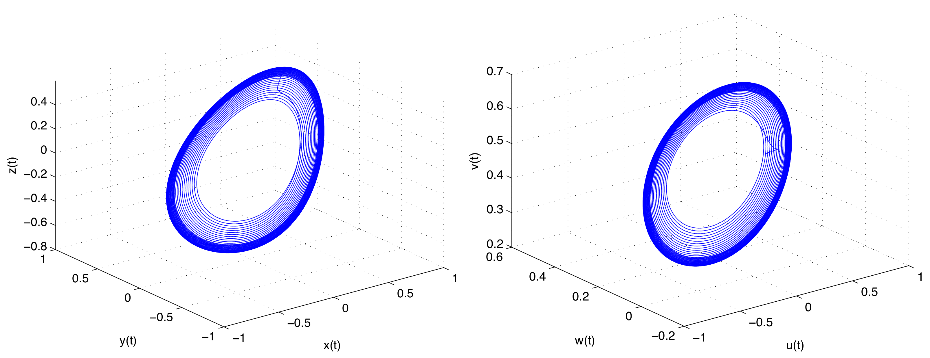
Figure 5 shows simulation results of the system (18) in state space, using numerical solution (19), for the parameters: , , , , , , , , , , , orders , initial conditions , step , and simulation time 500 s.
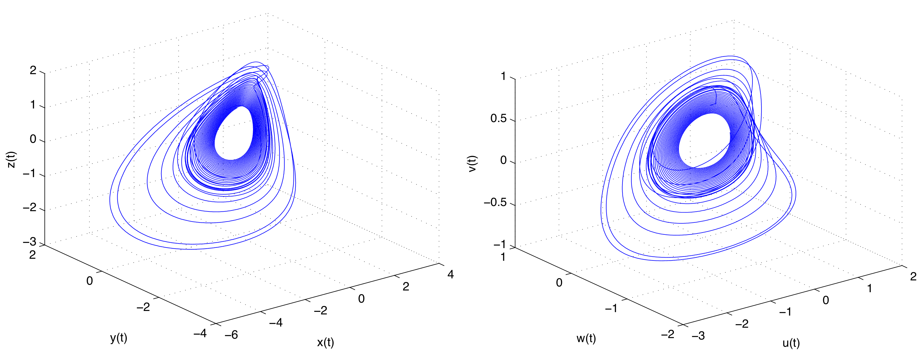
Figure 6 depicts the simulation results of the system (22) in state space, using numerical solution (23), for the parameters: , , , , , , , , , , , , , orders (capacitor), (memcapacitor), (meminductor), (memristor), , initial conditions , , , , , , step , and simulation time 500 s. The Lyapunov exponents of this system with the above parameters, computed according to the algorithm described in [39], have the following values: , which confirm the system is chaotic because at least one exponent is positive.
5. Discussion
Simulation results presented in this article confirm that new memory elements proposed only a few decades ago could be beneficial in new electronic circuit theory and practice. Moreover, a mathematical model for such elements should be a fractional order due to the memory of these parts. So far, it is possible only for a few well-known classical elements and the memristor [37]. Because the memory elements as memcapacitor and meminductor do not exist as a single electronic part, it is challenging to identify derivative order from experimental data. It will be possible when such elements are on sale. However, we may use an analogy with a classical capacitor and inductor to predict the real order in their mathematical models. Some experiments made by other authors confirm this theory [15,17].
Based on results depicted in Figure 5 and Figure 6, we can see that the new oscillator proposed in this article, depicted in Figure 4, may generate oscillation as well as chaotic behavior. Slight changes in parameters, orders, and initial conditions may produce different results. It could be significant in using such an oscillator with memory in secure communication, coding/decoding, and a new kind of memory circuits for future computers.
Here, we also present an idea for further work. Let us consider the circuit shown in Figure 7.
An important question is: Is it possible to generate chaos or hyperchaos using an electrical circuit, depicted in Figure 7, containing all known elements? It is an open problem.
6. Conclusions
This short article presents a new oscillator based on fractional-order elements with memory. We obtain a new circuit model described by the fractional differential equations.
Such a model was proposed as a numerical solution for simulation purposes as well as further investigation and analysis, for example, calculation of eigenvalues, Lyapunov exponents, Poincaré maps, and bifurcation diagrams. Moreover, the system (22) can work as a chaotic oscillator under appropriate parameters and initial values.
Such a combination of the fractional-order memory elements in the new oscillator circuit is presented for the first time. New is the part where an oscillator with three memory elements was proposed and its mathematical model and the numerical solution were derived. Both practical and theoretical relevance is significant for further circuit analysis.
Funding
This work was supported in part by the Slovak Grant Agency for Science under grant VEGA 1/0365/19 and by the Slovak Research and Development Agency under Contracts No. APVV-14-0892 and No. APVV-18-0526.
Institutional Review Board Statement
Not applicable.
Informed Consent Statement
Not applicable.
Data Availability Statement
Not applicable.
Conflicts of Interest
The author declares no conflict of interest.
References
- Yin, Z.; Tian, H.; Chen, G.; Chua, L.O. What are Memristor, Memcapacitor, and Meminductor? IEEE Trans. Circuits Syst. II Express Briefs 2015, 62, 402–406. [Google Scholar] [CrossRef] [Green Version]
- Chua, L.O. Memristor: The missing circuit element. IEEE Trans. Circuit Theory 1971, 18, 507–519. [Google Scholar] [CrossRef]
- Strukov, D.B.; Snider, G.S.; Stewart, D.R.; Williams, R.S. The missing memristor found. Nature 2008, 453, 80–83. [Google Scholar] [CrossRef] [PubMed]
- Chua, L.O.; Sung, M.K. Memristive devices and systems. Proc. IEEE 1976, 64, 209–223. [Google Scholar] [CrossRef]
- Ventra, M.D.; Pershin, Y.V.; Chua, L.O. Circuit elements with memory: Memristors, memcapacitors and meminductors. Proc. IEEE 2009, 97, 1717–1724. [Google Scholar] [CrossRef] [Green Version]
- Biolek, D.; Biolek, Z.; Biolkova, V. SPICE modeling of memristive, memcapacitative and meminductive systems. In Proceedings of the 2009 European Conference on Circuit Theory and Design, Antalya, Turkey, 23–27 August 2009; pp. 249–252. [Google Scholar] [CrossRef]
- Romero, F.J.; Ohata, A.; Toral-Lopez, A.; Godoy, A.; Morales, D.P.; Rodriguez, N. Memcapacitor and Meminductor Circuit Emulators: A Review. Electronics 2021, 10, 1225. [Google Scholar] [CrossRef]
- Khalil, N.A.; Fouda, M.E.; Said, L.A.; Radwan, A.G.; Soliman, A.M. A general emulator for fractional-order memristive elements with multiple pinched points and application. AEU—Int. J. Electron. Commun. 2020, 124, 153338. [Google Scholar] [CrossRef]
- Khalil, N.A.; Hezayyin, H.G.; Said, L.A.; Madian, A.H.; Radwan, A.G. Active emulation circuits of fractional-order memristive elements and its applications. AEU—Int. J. Electron. Commun. 2021, 138, 153855. [Google Scholar] [CrossRef]
- Cam Taskiran, Z.; Sagbas, M.; Ayten, U.; Sedef, H. A New Universal Mutator Circuit for Memcapacitor and Meminductor Elements. AEU—Int. J. Electron. Commun. 2020, 119, 153180. [Google Scholar] [CrossRef]
- Arena, P.; Caponetto, R.; Fortuna, L.; Porto, D. Nonlinear Noninteger Order Circuits and Systems: An Introduction; World Scientific: Singapore, 2000. [Google Scholar] [CrossRef]
- Elwakil, A.S. Fractional-order circuits and systems: An emerging interdisciplinary research area. IEEE Circuits Syst. Mag. 2010, 10, 40–50. [Google Scholar] [CrossRef]
- Schafer, I.; Kruger, K. Modelling of lossy coils using fractional derivatives. J. Phys. D Appl. Phys. 2008, 41, 045001. [Google Scholar] [CrossRef]
- Khalil, N.A.; Said, L.A.; Radwan, A.G.; Soliman, A.M. General fractional order mem-elements mutators. Microelectron. J. 2019, 90, 211–221. [Google Scholar] [CrossRef]
- Abdelouahab, M.S.; Lozi, R.; Chua, L.O. Memfractance: A Mathematical Paradigmfor Circuit Elements with Memory. Int. J. Bifurc. Chaos Appl. Sci. Eng. 2014, 24, 1430023–1430029. [Google Scholar] [CrossRef] [Green Version]
- Coopmans, C.; Petráš, I.; Chen, Y. Analogue Fractional-Order Generalized Memristive Devices. In Proceedings of the International Design Engineering Technical Conferences and Computers and Information in Engineering Conference, San Diego, CA, USA, 30 August–2 September 2009; Volume 4, pp. 1127–1136. [Google Scholar] [CrossRef]
- Guo, Z.; Si, G.; Diao, L.; Jia, L.; Zhang, Y. Generalized modeling of the fractional-order memcapacitor and its character analysis. Commun. Nonlinear Sci. Numer. Simul. 2018, 59, 177–189. [Google Scholar] [CrossRef]
- Yang, N.N.; Xu, C.; Wu, C.; Jia, R.; Liu, C. Fractional-order cubic nonlinear flux-controlled memristor: Theoretical analysis, numerical calculation and circuit simulation. Nonlinear Dyn. 2019, 97, 33–44. [Google Scholar] [CrossRef]
- Zhou, P.; Tang, J. Clarify the physical process for fractional dynamical systems. Nonlinear Dyn. 2020, 100, 2353–2364. [Google Scholar] [CrossRef]
- Tenreiro Machado, J.A.; Lopes, A.M. Multidimensional scaling locus of memristor and fractional order elements. J. Adv. Res. 2020, 25, 147–157. [Google Scholar] [CrossRef]
- Tenreiro Machado, J. Fractional generalization of memristor and higher order elements. Commun. Nonlinear Sci. Numer. Simul. 2013, 18, 264–275. [Google Scholar] [CrossRef] [Green Version]
- Petráš, I. Fractional-Order Nonlinear Systems; Springer: New York, NY, USA, 2011. [Google Scholar] [CrossRef] [Green Version]
- Caponetto, R.; Dongola, G.; Fortuna, L.; Petráš, I. Fractional Order Systems: Modeling and Control Applications; World Scientific: Singapore, 2010. [Google Scholar] [CrossRef]
- Podlubny, I. Fractional Differential Equations; Academic Press: San Diego, CA, USA, 1999. [Google Scholar]
- Oldham, K.B.; Spanier, J. The Fractional Calculus; Academic Press: New York, NY, USA, 1974. [Google Scholar]
- Westerlund, S.; Ekstam, L. Capacitor theory. IEEE Trans. Dielectr. Electr. Insul. 1994, 1, 826–839. [Google Scholar] [CrossRef]
- Lopez, C.S.; Gomez, V.H.C.; Aguilar, M.A.C.; Lopez, F.E.M. PID controller design based on memductor. Int. J. Electron. Commun. 2019, 101, 9–14. [Google Scholar] [CrossRef]
- Pershin, Y.V.; Ventra, M.D. Memristive circuits simulate memcapacitors and meminductors. Electron. Lett. 2010, 46, 517–518. [Google Scholar] [CrossRef] [Green Version]
- Ma, X.; Mou, J.; Liu, J.; Ma, C.; Yang, F.; Zhao, X. A novel simple chaotic circuit based on memristor–memcapacitor. Nonlinear Dyn. 2020, 100, 2859–2876. [Google Scholar] [CrossRef]
- Innocenti, G.; Liu, X.; Bi, X.; Yan, H.; Mou, J. A Chaotic Oscillator Based on Meminductor, Memcapacitor, and Memristor. Complexity 2021, 2021, 7223557. [Google Scholar] [CrossRef]
- Wang, X.; Yu, J.; Jin, C.; Iu, H.H.C.; Yu, S. Chaotic oscillator based on memcapacitor and meminductor. Nonlinear Dyn. 2019, 96, 161–173. [Google Scholar] [CrossRef]
- Radwan, A.G.; Fouda, M.E. On the Mathematical Modeling of Memristor, Memcapacitor, and Meminductor; Springer: Berlin/Heidelberg, Germany, 2015. [Google Scholar]
- Petráš, I.; Chen, Y. Fractional-order circuit elements with memory. In Proceedings of the 13th International Carpathian Control Conference (ICCC), High Tatras, Slovakia, 28–31 May 2012; pp. 552–558. [Google Scholar] [CrossRef]
- Itoh, M.; Chua, L.O. Memristor oscillation. Int. J. Bifurcat. Chaos Appl. Sci. Eng. 2008, 18, 3183–3206. [Google Scholar] [CrossRef]
- Petráš, I. Fractional-order memristor-based Chua’s circuit. IEEE Trans. Circuits Syst. II Express Briefs 2010, 57, 975–979. [Google Scholar] [CrossRef]
- Westerlund, S. Dead Matter Has Memory! Causal Consulting: Kalmar, Sweden, 2002. [Google Scholar]
- Wang, S.F.; Ye, A. Dynamical Properties of Fractional-Order Memristor. Symmetry 2020, 12, 437. [Google Scholar] [CrossRef] [Green Version]
- Petráš, I. “Comments on “Chaotic oscillator based on memcapacitor and meminductor” (Nonlinear Dyn, DOI: 10.1007/s11071-019-04781-5). Nonlinear Dyn. 2020, 102, 2945–2950. [Google Scholar] [CrossRef]
- Wolf, A.; Swift, J.B.; Swinney, H.L.; Vastano, J.A. Determining Lyapunov exponents from a time series. Phys. D Nonlinear Phenom. 1985, 16, 285–317. [Google Scholar] [CrossRef] [Green Version]

Figure 2.
Chaotic oscillator circuit based on two memory elements [31].
Figure 2.
Chaotic oscillator circuit based on two memory elements [31].

Figure 3.
One-scroll attractors of the system (18) in state space (left) and state plane (right).
Figure 3.
One-scroll attractors of the system (18) in state space (left) and state plane (right).

Figure 4.
Chaotic oscillator circuit based on three memory elements.

Figure 5.
Orbits of the fractional-order oscillator (22) in state spaces , , respectively.
Figure 5.
Orbits of the fractional-order oscillator (22) in state spaces , , respectively.

Figure 6.
One-scroll attractors of the system (22) in state space (left) and (right).
Figure 6.
One-scroll attractors of the system (22) in state space (left) and (right).

Figure 7.
New oscillator circuit based on all known electrical elements.

Publisher’s Note: MDPI stays neutral with regard to jurisdictional claims in published maps and institutional affiliations. |
© 2022 by the author. Licensee MDPI, Basel, Switzerland. This article is an open access article distributed under the terms and conditions of the Creative Commons Attribution (CC BY) license (https://creativecommons.org/licenses/by/4.0/).
Share and Cite
MDPI and ACS Style
Petráš, I. Oscillators Based on Fractional-Order Memory Elements. Fractal Fract. 2022, 6, 283. https://0-doi-org.brum.beds.ac.uk/10.3390/fractalfract6060283
AMA Style
Petráš I. Oscillators Based on Fractional-Order Memory Elements. Fractal and Fractional. 2022; 6(6):283. https://0-doi-org.brum.beds.ac.uk/10.3390/fractalfract6060283
Chicago/Turabian StylePetráš, Ivo. 2022. "Oscillators Based on Fractional-Order Memory Elements" Fractal and Fractional 6, no. 6: 283. https://0-doi-org.brum.beds.ac.uk/10.3390/fractalfract6060283