Article

Asymptotic and Finite-Time Synchronization of Fractional-Order Memristor-Based Inertial Neural Networks with Time-Varying Delay

1
School of Finance and Mathematics, Huainan Normal University, Huainan 232038, China
2
School of Computer Science, Huainan Normal University, Huainan 232038, China
*
Author to whom correspondence should be addressed.
Submission received: 15 May 2022 / Revised: 17 June 2022 / Accepted: 21 June 2022 / Published: 23 June 2022

Abstract

:
This paper emphasized on studying the asymptotic synchronization and finite synchronization of fractional-order memristor-based inertial neural networks with time-varying latency. The fractional-order memristor-based inertial neural network model is offered as a more general and flexible alternative to the integer-order inertial neural network. By utilizing the properties of fractional calculus, two lemmas on asymptotic stability and finite-time stability are provided. Based on the two lemmas and the constructed Lyapunov functionals, some updated and valid criteria have been developed to achieve asymptotic and finite-time synchronization of the addressed systems. Finally, the effectiveness of the proposed method is demonstrated by a number of examples and simulations.

1. Introduction

In 1986, Babcock and his collaborator Westervelt introduced inductance into the neural circuit model to reveal the existence of inertia in the model, and the inertial neural network described by higher-order differential equations came into being [1]. Due to the strong physical meaning and biological background of inertial resistance, for example, the axon of squid can be realized by designing an inductance, and the membrane semicircular canal of hair cells can also be realized by an equivalent inductive circuit [2,3]. People usually call this neural network model with added inductance an inertial neural network. From the point of view of physical meaning and mathematical model, the inertial neural network model is essentially a network model with damping approaching infinity. When the damping value exceeds the critical state, the dynamic properties of each neuron in the network model will fundamentally change, which provides us with a powerful tool to generate complex dynamic behaviors such as chaos and bifurcation. At present, many research results have been achieved on the neural network with inertial term, mainly including the following: exponential stability of inertial neural network [4], anti-periodic solution [5], global stability [6], global convergence analysis [7], exponential dissipativeness [8], stability of Cohen–Grossberg Neural Networks [9], global asymptotic stability and robust stability [10], finite time synchronization [11], fixed time synchronization [12], and exponential synchronization [13].
On the other hand, memory resistors have attracted extensive interest because of their prospective applications, such as new generation computers and AI computers [14]. A memristor-based neural network in which resistors replace circuit implementations, and they are ideally suited for mimicking the human brain due to the features of the memristor [15]. Due to its widespread applicability, the analysis of dynamic behaviors for such memristor-based neural networks has attracted considerable interest in recent years [16,17,18]. Furthermore, fractional-order calculus could be traced back three hundred years as an extension of integer derivatives and integral to arbitrary order [19]. Compared with classical integer-order systems, dynamic systems in the real world can be better characterized by fractional-order systems because fractional-order differentiation considers the current state and the history of its prior states [20,21]. In other words, fractional-order systems possess memory and heredity. Due to its infinite memory function and genetic characteristics, it has been introduced into the neural network, and the so-called fractional-order neural network is generated [22,23].
Based on the relevant literature, it is found that inertial neural networks, memristive-based neural networks, and fractional-order neural networks have received the attention and research of many scholars, and there have been relatively rich research results around their respective dynamic properties. However, so far, few researchers have combined inertial terms, memristors, and fractional-order systems to study neural networks. Since inertial, memristor and fractional-order systems have specific physical meanings and biological backgrounds in practical applications, the combination of the three can simulate more complex network systems, which is also the enrichment and improvement of existing neural network theories. In addition, due to the limited switching speed of amplifiers in neural networks and the limited signal transmission time in biological networks, the generation of time delays is usually unavoidable: for example, multiple time delays [24], time-varying delays [25], mixed time delays [26], bounded distributed delays [27], and unbounded delays [28]. It has a significant impact on the dynamic properties of neural networks, such as causing network vibration, bifurcation, instability, and other phenomena [29]. Therefore, it is more practical to study the dynamic behavior of neural networks with time delay.
Recently, fractional-order neural networks with inertial terms have received extensive attention from many scholars. Different from the traditional integer-order inertial neural network, the fractional-order inertial neural network model can more truly reflect the dynamic behavior of the real world. Therefore, the research on the dynamics of the fractional-order inertial neural network has theoretical significance and practical value. Gu et al. [30] discussed the stability and synchronization control method of Riemann–Liouville time-delayed inertial fractional order neural network based on the feedback control method. Li et al. [31] established a Cohen–Grossberg inertial fractional neural network model and revealed the boundedness of the Cohen-Grossberg inertial fractional neural network and the Mittag-Leffler synchronization law by analyzing the model. Ke et al. [32] discussed the stability of a class of time-delayed inertial fractional-order neural networks and provided sufficient conditions for asymptotic x-periodicity and Mittag–Leffler stability. The Riemann–Liouville delay fractional-order neural network model studied by Zhang et al. [33] has two inertial terms, and gives a controller design method to achieve master-slave system synchronization. Yang et al. [34] studied the quasi-synchronization problem of inertial memristive fractional-order delay neural network based on Razumikhin technique. To counteract the fractional derivative term from 0 to 1, this study develops a special controller and a set of sufficient conditions for the synchronization of fractional memristive inertial neural networks. However, the existing literature either studies the synchronization control problem of fractional-order inertial neural networks in the sense of Riemann–Liouville or the quasi-synchronization problem of inertial memristive fractional-order neural networks.
To the best of our knowledge, asymptotic and finite-time synchronization of delayed inertial fractional-order memristive neural networks has not been previously performed, which was the impetus for our study. This study’s purpose is to establish some innovative asymptotic and finite-time synchronization criteria for delayed inertial fractional-order memristive neural networks. The following is a summary of this article’s primary contributions:
  • The Caputo fractional-order memristor-based inertial network model is constructed. Compared with the inertial integer-order neural network, the Caputo fractional-order memristor-based inertial network model can be widely and flexibly used. In addition, the advantage of this model is that it has a practical engineering background and is relatively easy to implement in engineering.
  • By utilizing the properties of fractional calculus, two lemmas on asymptotic stability and finite-time stability are given, which are crucial to the proofs of our principal theorems.
  • Based on the two proposed lemmas and Lyapunov direct methods, some new asymptotic and finite-time synchronization control strategies for inertial memristor-based Caputo fractional-order neural networks are proposed.
  • The direct analysis method is adopted to analyze the dynamic performance of the inertial system without using the reduced-order method based on variable substitution, which not only avoids increasing the system’s dimension, thereby increasing the difficulty of analysis, but also avoids the loss of system inertia; thus, it has more important practical significance.
The structure of this paper is as described below. Section 2 presents the model formulation and some preliminary work. Section 3 develops new asymptotic and finite-time synchronization criteria for fractional-order memristor-based inertial neural networks with time-varying latency. In Section 4, several examples and their simulations are provided to illustrate the effectiveness of our theoretical results. Finally, a brief discussion and future research topics are provided in Section 5.

2. Problem Statement and Preliminaries

2.1. Basic Knowledge

This section introduces some related mathematical concepts, including the definition of fractional calculus, the theory of fractional differential equations, the solution of discontinuous fractional differential equations in the sense of Filipov [35], and some model assumptions required.
Definition 1
([16]). Define the fractional integral for an arbitrary function g ( t ) as follows:
D t β g ( t ) = 1 Γ ( β ) t 0 t ( t s ) β 1 g ( s ) d s ,
where t > t 0 , β > 0 .
Definition 2
([16]). Define the Caputo fractional derivative for an arbitrary function g ( t ) as follows:
D t β g ( t ) = 1 Γ ( n β ) t 0 t ( t s ) n β 1 g ( n ) ( s ) d s ,
where n 1 β < n , t > t 0 . If 0 < β < 1 , then we have the following.
D t β g ( t ) = 1 Γ ( 1 β ) t 0 t g ( s ) ( t s ) β d s .
Lemma 1
([19]). If p , q R , and β > 0 , then Equation (4) holds.
D t β ( p x 1 ( t ) + q x 2 ( t ) ) = p D t β x 1 ( t ) + q D t β x 2 ( t ) .
Lemma 2
([19]). If α , β > 0 , x ( t ) C 1 [ 0 , T ] , then we have the following.
D t α D t β x ( t ) = D t α β x ( t ) .
Lemma 3
([19]). If D t β g ( t ) is integrable, then we have the following.
D t β D t β g ( t ) = g ( t ) i = 0 k 1 g ( i ) ( t 0 ) i ! t t 0 i
Especially, for 0 < β 1 , we have the following.
D t β D t β g ( t ) = g ( t ) g ( t 0 )
Lemma 4.
Let x ( t ) R n be a vector of differentiable function. If a continuous function V : [ t 0 , ) × R n R satisfies the following:
D t α V ( t , x ( t ) ) ρ V ( t , x ( t ) )
then the following is obtained
V ( t , x ( t ) ) V ( t 0 , x ( t 0 ) ) E α ρ t t 0 α
where 0 < α < 1 , ρ is a positive constant.
Proof of Lemma 4. 
There exists a nonnegative function M ( t ) satisfying the follow equation
D t α V ( t , x ( t ) ) + ρ V ( t , x ( t ) ) + M ( t ) = 0
Taking the Laplace transform of (10), we obtain the following:
s α V ( s ) s α 1 V ( t 0 , x ( t 0 ) ) + ρ V ( s ) + M ( s ) = 0
where V ( s ) = L ( V ( t , x ( t ) ) ) , M ( s ) = L ( M ( t ) ) .
The following is then the case.
V ( s ) = s α 1 V ( t 0 , x ( t 0 ) ) M ( s ) s α + α
Taking the inverse Laplace transform of (12), we obtain the following:
V ( t , x ( t ) ) = V ( t 0 , x ( t 0 ) ) E α ρ t t 0 α M ( t ) t t 0 α 1 E α , α ρ t t 0 α
where E α ( · ) , E α , α ( · ) are Mittag–Leffler functions, and * is the convolution operator.
Since M ( t ) , t t 0 α 1 , E α , α ρ t t 0 α are all nonnegative functions, we obtain the following.
V ( t , x ( t ) ) V ( t 0 , x ( t 0 ) ) E α ρ t t 0 α
The proof is completed. □
Lemma 5.
Let x ( t ) R n be a vector of differentiable function. If the positive-definite continuous function V : [ t 0 , ) × R n R + can make the following inequality hold:
D t α V ( t , x ( t ) ) μ
then we have the following:
V ( t , x ( t ) ) V ( t 0 , x ( t 0 ) ) μ t t 0 α Γ 1 + α , t 0 t t 1
and V ( t , x ( t ) ) = 0 for all t t 1 with t 1 is given by the following
t 1 = t 0 + Γ 1 + α V ( t 0 , x ( t 0 ) ) μ 1 α
where 0 < α < 1 , μ is a positive constant.
Proof of Lemma 5. 
It is clear that there exists a non-negative function M ( t ) such that the following equation holds
D t α V ( t , x ( t ) ) + M ( t ) + μ = 0
It follows from Lemma 3 and Definition 1 and (18) that the following is the case.
V ( t , x ( t ) ) = V ( t 0 , x ( t 0 ) ) D t α M ( t ) D t α μ = V ( t 0 , x ( t 0 ) ) 1 Γ ( α ) t 0 t M ( s ) t s 1 α d s 1 Γ ( α ) t 0 t μ t s 1 α d s V ( t 0 , x ( t 0 ) ) μ t t 0 α Γ 1 + α
Denote the following.
Ψ ( t ) = V ( t 0 , x ( t 0 ) ) μ t t 0 α Γ 1 + α
Evidently, Ψ ( t ) is a strictly decreasing function with respect to t; hence, we have Ψ ( t ) = 0 if and only if the following is the case:
t 1 = t 0 + Γ 1 + α V ( t 0 , x ( t 0 ) ) μ 1 α
and Ψ ( t ) 0 for all t 0 t t 1 . Since V ( t , x ( t ) ) Ψ ( t ) 0 for all t 0 t t 1 , and V ( t , x ( t ) ) is a nonnegative function, we obtain V ( t , x ( t ) ) = 0 for all t 0 t t 1 .
The proof is completed. □

2.2. Problem Formulation

The following fractional order delayed memristor-based inertial neural network is discussed in this part:
D t α x i ( t ) = a i D t β x i ( t ) b i x i ( t ) + j = 1 n c i j x j ( t ) f j x j ( t ) + j = 1 n d i j x j ( t ) g j x j t τ j ( t ) + I i ( t ) , t > 0
where 0 < β < α 1 , i = 1 , 2 , , n , a i , b i are constants, x i ( t ) represents the state of ith neuron, f i , g i are activation functions, τ j ( t ) is the time-varying delay and satisfies 0 τ j ( t ) τ j , and I i ( t ) is the external input. c i j x j ( t ) , d i j x j ( t ) represent the memristor connection weights, and they are characterized by the following equations:
c i j x j ( t ) = c i j * , x j ( t ) X j c i j * * , x j ( t ) > X j d i j x j ( t ) = d i j * , x j ( t ) X j d i j * * , x j ( t ) > X j
where X j > 0 is the switching value of memristor, and c i j * , c i j * * , d i j * , d i j * * are constants.
The initial values of system (22) are provided by x i ( s ) = ψ i ( s ) , D t β x i ( s ) = ϑ i ( s ) , τ j ( t ) s 0 .
Similarly, the response system of (22) is shown below:
D t α y i ( t ) = a i D t β y i ( t ) b i y i ( t ) + i = 1 n c i j y j ( t ) f j y j ( t ) + j = 1 n d i j y j ( t ) g j y j t τ j ( t ) + I i ( t ) + u i ( t ) , t > 0
where u i ( t ) is the control input, the initial conditions of system (23) are y i ( s ) = ω i ( s ) , D t β y i ( s ) = γ i ( s ) , τ j ( t ) s 0 , and the memristor connection weights can be described as the following equations.
c i j y j ( t ) = c i j * , y j ( t ) Y j c i j * * , y j ( t ) > Y j d i j y j ( t ) = d i j * , y j ( t ) Y j d i j * * , y j ( t ) > Y j
Remark 1.
If α = β , then (22) is the following system.
D t α x i ( t ) = b i a i + 1 x i ( t ) + 1 a i + 1 j = 1 n c i j ( x j ( t ) ) f j ( x j ( t ) ) + 1 a i + 1 j = 1 n d i j ( x j ( t ) ) g j ( x j ( t τ j ( t ) ) ) + 1 a i + 1 I i ( t ) .
If α < β , then (22) is the following system.
D t β x i ( t ) = 1 a i D t α x i ( t ) b i a i x i ( t ) + 1 a i j = 1 n c i j ( x j ( t ) ) f j ( x j ( t ) ) + 1 a i j = 1 n d i j ( x j ( t ) ) g j ( x j ( t τ j ( t ) ) ) + 1 a i I i ( t ) .
Therefore, the case α > β is only concerned.
Our target is to design a proper controller to make (22) and (23) synchronous. However, system (22) and system (23) are systems with a discontinuous right-hand side. Therefore, before designing the controller, we need to transform them into continuous systems according to the differential theory and set-valued map:
D t α x i ( t ) a i D t β x i ( t ) b i x i ( t ) + j = 1 n co c i j x j ( t ) f j x j ( t ) + j = 1 n co d i j x j ( t ) g j x j t τ j ( t ) + I i ( t ) , t > 0
D t α y i ( t ) a i D t β y i ( t ) b i y i ( t ) + j = 1 n c o c i j y j ( t ) f j y j ( t ) + i = 1 n c o d i j y j ( t ) g j y j t τ j ( t ) + I i ( t ) + u i ( t ) , t > 0
where we have the following.
c o c i j x j ( t ) = c i j * , x j ( t ) < X j c i j , c ¯ i j , x j ( t ) = X j c i j * * , x j ( t ) > X j c o d i j x j ( t ) = d i j * , x j ( t ) < X j d ̲ i j , d ¯ i j , x j ( t ) = X j d i j * , x j ( t ) > X j
c o c i j y j ( t ) = c i j * , y j ( t ) < Y j c i j , c ¯ i j , y j ( t ) = Y j c i j * * , y j ( t ) > Y j c o d i j y j ( t ) = d i j * , y j ( t ) < Y j d ̲ i j , d ¯ i j , y j ( t ) = Y j d i j * * , y j ( t ) > Y j
Here, c ̲ i j = min { c i j * , c i j * * } , c ¯ i j = max { c i j * , c i j * * } , d ̲ i j = min { d i j * , d i j * * } , d ¯ i j = max { d i j * , d i j * * } , c i j = max { | c ̲ i j | , | c ¯ i j | } , d i j = max { | d ̲ i j | , | d ¯ i j | } . Moreover, there exists h i j ( x j ( t ) ) co c i j x j ( t ) , p i j ( x j ( t ) ) co d i j x j ( t ) , h ¯ i j ( y j ( t ) ) co c i j y j ( t ) , p ¯ i j ( y j ( t ) ) co d i j y j ( t ) such that the following is the case.
D t α x i ( t ) = a i D t β x i ( t ) b i x i ( t ) + j = 1 n h i j x j ( t ) f j x j ( t ) + j = 1 n p i j x j ( t ) g j x j t τ j ( t ) + I i ( t ) , t > 0
D t α y i ( t ) = a i D t β y i ( t ) b i y i ( t ) + j = 1 n h ¯ i j y j ( t ) f j y j ( t ) + j = 1 n p ¯ i j y j ( t ) g j y j t τ j ( t ) + I i ( t ) + u i ( t ) , t > 0
We define the error as e i ( t ) = y i ( t ) x i ( t ) ; consequently, the error system can be characterized using the following equation:
D t α e i ( t ) = a i D t β e i ( t ) b i e i ( t ) + j = 1 n h i j y j ( t ) f j y j ( t ) h i j x j ( t ) f j x j ( t ) + i = 1 n p ¯ i j y j ( t ) g j y j t τ j ( t ) p i j x j ( t ) g j x j t τ j ( t ) + u i ( t ) , t > 0
where the initial value is e i ( s ) = ω i ( s ) ψ i ( s ) = κ i ( s ) , D t β e i ( s ) = γ i ( s ) ϑ i ( s ) = υ i ( s ) . We define a kind of norm as sup | e i ( s ) | = | κ i | .
In order to guarantee the uniqueness and existence of the solutions of inertial time-delayed fractional order memristor-based neural network (22) or fractional-order differential inclusion (28), the following assumption should be imposed on activation f i and g i .
Assumption 1.
For l , m R , there exists constant F i , G i > 0 , i = 1 , 2 , , n , such that the following inequalities hold.
f i ( l ) f i ( m ) F i l m g i ( l ) g i ( m ) G i l m
Assumption 2.
The activation function f i , g i are bounded; in other words, there exist constants M i , N i > 0 satisfying the following inequality.
f i ( x ) < M i g i ( x ) < N i
Remark 2.
Assumption 2 is a general assumption for synchronization of memristive fractional neural network. Many common activation functions, such as hyperbolic tangent function f ( x ) = tanh ( x ) , ramp function f ( x ) = 1 2 ( | x + 1 | | x 1 | ) , and Sigmoid function f ( x ) = 1 1 + e x , satisfy Assumption 2. In addition, when constructing multi-layer neural networks, the bounded activation function values, i.e., the bounded outputs of neurons, can easily serve as the inputs of other layers. Hence, Assumption 2 is reasonable.

3. Main Results

In this part, the asymptotic and finite-time synchronization criteria for inertial memristive fractional delayed neural networks are provided.
The following controller is introduced below:
u i ( t ) = k i e i ( t ) q i a i D t β α e i ( t ) δ i
where k i , q i , δ i are control gains to be designed later.

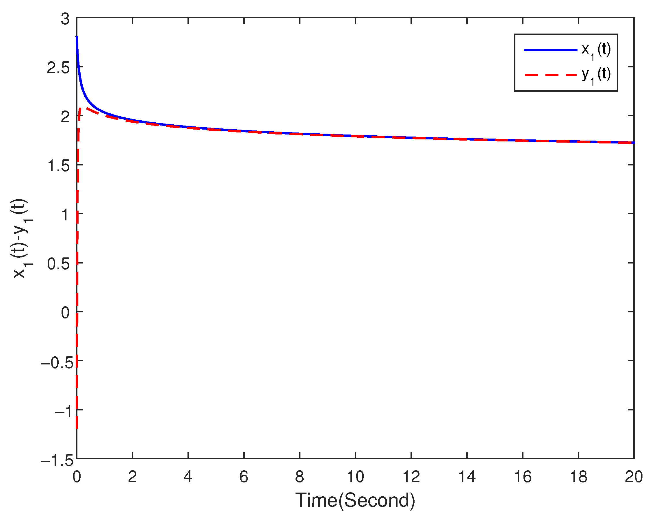
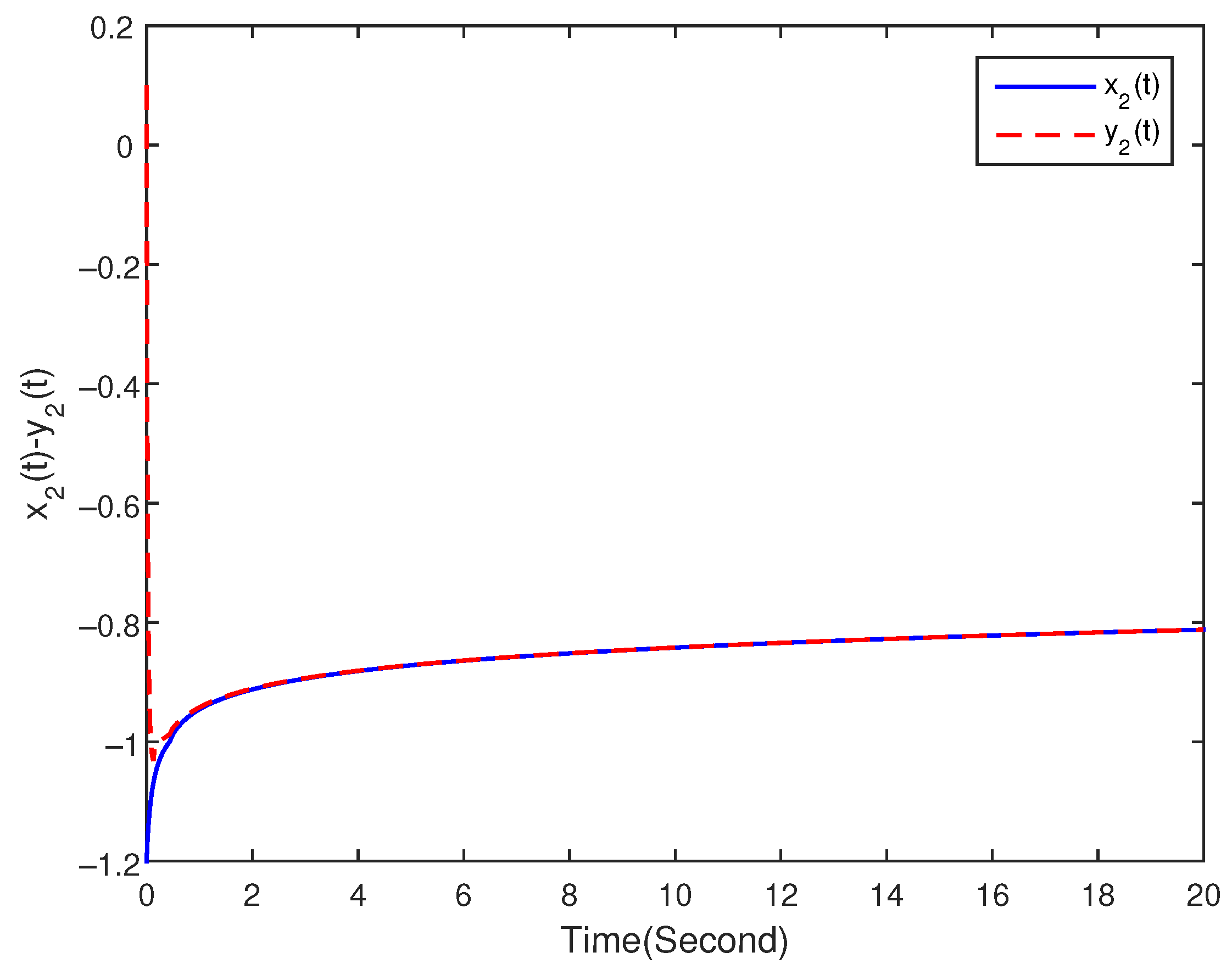
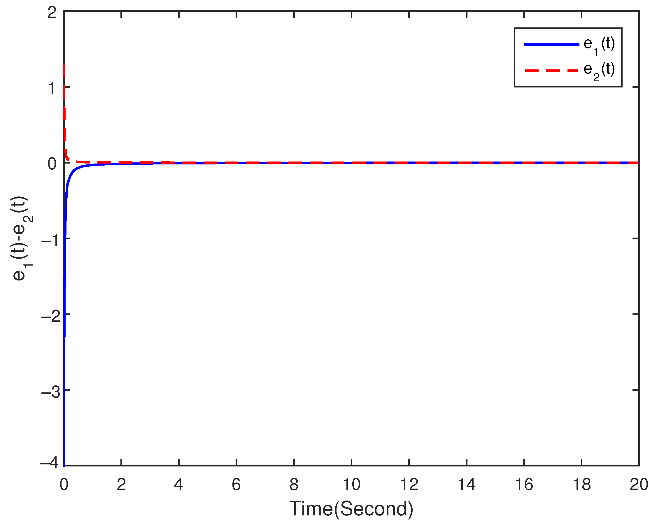
3.1. Asymptotic Synchronization

Theorem 1.
If Assumptions 1 and 2 are fulfilled, and control parameters k i , q i , δ i satisfy the following conditions:
k i > b i + j = 1 n c i j F j + j = 1 n d i j G j
q i = b i + k i j = 1 n c i j F j j = 1 n d i j G j
δ i = j = 1 n L a + L b + d i j G j κ j
then systems (22) and (23) can achieve asymptotic synchronization under controller (31).
Proof of Theorem 1. 
The following Lyapunov function is considered.
V ( t ) = i = 1 n e i ( t ) + i = 1 n a i D t β α e i ( t )
In light of Lemmas 1 and 2, we obtain the following:
D t α V ( t ) = D t α i = 1 n e i ( t ) + D t α i = 1 n a i D t β α e i ( t ) = i = 1 n D t α e i ( t ) + a i D t β e i ( t ) i = 1 n sgn e i ( t ) D t α e i ( t ) + a i D t β e i ( t )
where s g n ( · ) is the symbolic function. On the basis of system (9), we have the following.
D t α V ( t ) i = 1 n sgn e t ( t ) b i e i ( t ) + j = 1 n h ¯ i j y j ( t ) f j y j ( t ) h i j x j ( t ) f j x j ( t ) + j = 1 n p ¯ i j y j ( t ) g j y j t τ j ( t ) p i j x j ( t ) g j x j t τ j ( t ) + u i ( t )
If Assumption 2 holds, we have the following:
h ¯ i j y j ( t ) f j y j ( t ) h i j x j ( t ) f j x j ( t ) = h ¯ i j y j ( t ) f j y j ( t ) h ¯ i j y j ( t ) f j x j ( t ) + h ¯ i j y j ( t ) h i j x j ( t ) f j x j ( t )
in which the following is the case.
h ¯ i j y j ( t ) f j y j ( t ) h ¯ i j y j ( t ) f j x j ( t ) c i j F j e j ( t ) h ¯ i j y j ( t ) h i j x j ( t ) f j x j ( t ) c i j * c i j * * M j
Let L a = c i j * c i j * * M j ; thus, we have the following.
h ¯ i j y j ( t ) f j y j ( t ) h i j x j ( t ) f j x j ( t ) c i j F j e j ( t ) + L a
Similarly, let L b = d i j * d i j * * N j ; then, we have the following.
p ¯ i j y j ( t ) g j y j t τ j ( t ) p i j x j ( t ) g j x j t τ j ( t ) c i j F j e j ( t ) + L b
From the above, we can deduce the following.
D t α V ( t ) i = 1 n b i k i e i ( t ) q i a i D t β α e i ( t ) + j = 1 n c i j F j e j ( t ) + j = 1 n d i j G j e j t τ j ( t ) + j = 1 n L a + L b δ i }
By using Razumikhin technology [36], we have the following.
e j t τ j ( t ) sup τ j s 0 e j ( s ) + e j ( t ) = κ j + e j ( t )
Thus, the following is the case.
D t α V ( t ) i = 1 n b i k i + j = 1 n c i j F j + j = 1 n d i j G j e i ( t ) q i a i D t β α e i ( t ) + j = 1 n L a + L b + d i j G j κ j δ i = i = 1 n b i k i + j = 1 n c i j F j + j = 1 n d i j G j D t α e i ( t ) + a i D t β e i ( t ) + i = 1 n j = 1 n L a + L b + d i j G j κ j δ i
Consequently, given conditions (32)–(34), it follows that the following is the case:
D t α V ( t ) = D t α i = 1 n V i ( t ) i = 1 n q i V i ( t )
which yields the following.
D t α V i ( t ) q i V i ( t )
According to Lemma 4, systems (22) and (23) achieve asymptotic synchronization.
The proof is completed. □
Remark 3.
In order to improve the network’s computing capacity, parallel capacity, and adaptive capacity, our paper combines a inertial fractional neural networks with a memristor to propose an inertial memristive fractional neural networks. For the discontinuity brought about by the memristor, the set-valued mapping theory was used to solve it. In addition, in order to eliminate the delay term e j ( t τ j ( t ) ) , Razumikhin technology is applied to convert the delay term e j ( t τ j ( t ) ) to non-delay term e j ( t ) .
Remark 4.
Most of the results are used to transform the second-order inertial model into a first-order differential system by using appropriate variable substitution. However, this method not only increases the dimension of the system but also renders theoretical analysis more difficult, and the reduced order differential equation loses the characteristics of the original inertial term. This paper adopts the direct analysis method to analyze the dynamic performance of the inertial system without using the reduced-order variable substitution method; thus, it has more important practical significance.

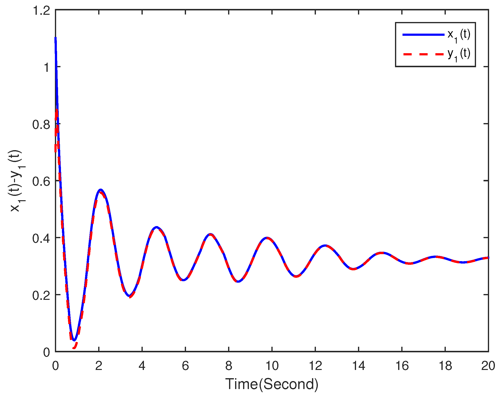
3.2. Finite-Time Synchronization

Theorem 2.
If Assumptions 1 and 2 are fulfilled and control parameters k i , q i , δ i satisfy the following conditions:
k i > b i + j = 1 n c i j F j + j = 1 n d i j G j
q i = b i + k i j = 1 n c i j F j j = 1 n d i j G j
δ i > j = 1 n L a + L b + d i j G j κ j
then, under controller (31), systems (22) and (23) can achieve finite synchronization, with settling time t 1 given by the following.
t 1 = t 0 + Γ 1 + α V ( t 0 , x ( t 0 ) ) μ 1 α
Proof of Theorem 2. 
We can obtain similar results from Theorem 1.
D t α V ( t ) i = 1 n b i k i + j = 1 n c i j F j + j = 1 n d i j G j e i ( t ) q i a i D t β α e i ( t ) + j = 1 n L a + L b + d i j G j κ j δ i
Denote the following.
μ i = δ i j = 1 n L a + L b + d i j G j κ j
Then, it follows from the conditions (43)–(45) that the following is the case.
D t α V ( t ) = D t α i = 1 n V i ( t ) i = 1 n q i V i ( t ) μ i μ i
According to Lemma 5, systems (22) and (23) achieve finite-time synchronization when the settling time is given by the following.
t 1 = t 0 + Γ 1 + α V ( t 0 , x ( t 0 ) ) μ 1 α
This completes the proof. □
Remark 5.
It should be noted that the asymptotic and finite-time synchronization analysis of the original system is converted into the asymptotic and finite-time stability analysis of its error system. This is also the reason why two lemmas are provided at the beginning of this article.
Remark 6.
Time delays may cause oscillation, bifurcation, and chaos. However, it is inevitable that time delay, including multiple delays, mixed delays, time-varying delays, bounded distributed delays, and unbounded delays, exists in the electronic implementation of neural works due to various reasons. Therefore, the investigation on time-delay neural networks is not only significant for theory research but also valuable in practice.

4. Numerical Examples

To illustrate the validity of the proposed theoretical results, in this part, we present two simulation examples.
Example 1.
Consider the first inertial memristive fractional delayed neural network as follows:
D t α x i ( t ) = a i D t β x i ( t ) b i x i ( t ) + j = 1 2 c i j x j ( t ) f j x j ( t ) + j = 1 2 d i j x j ( t ) g j x j t τ j ( t ) + I i ( t ) , t > 0
where the activation functions are f j = g j = | x + 1 | | x 1 | 2 , and the delay is τ j ( t ) = 0.1 sin ( t ) + 0.1 .
The system parameters are chosen as follows.
a 1 = 4.5 , a 2 = 4.5 b 1 = 1.8 , b 2 = 1.8 I 1 = 0 , I 2 = 0 α = 0.90 , β = 0.15
The initial values are as follows.
x 1 ( 0 ) = 2.8 , x 2 ( 0 ) = 1.2 D t β x 1 ( 0 ) = 3.5 , D t β x 2 ( 0 ) = 2.2
The connection weights are as follows.
c 11 = 1.20 , x 1 1 0.90 , x 1 > 1 c 12 = 0.30 , x 2 1 0.16 , x 2 > 1 c 21 = 0.50 , x 1 1 0.80 , x 1 > 1 c 22 = 0.09 , x 2 1 0.25 , x 2 > 1 d 11 = 0.48 , x 1 1 0.34 , x 1 > 1 d 12 = 0.36 , x 2 1 0.56 , x 2 > 1 d 21 = 0.65 , x 1 1 0.80 , x 1 > 1 d 22 = 0.60 , x 2 1 0.40 , x 2 > 1
The response system of (51) is shown below.
D t α y i ( t ) = a i D t β y i ( t ) b i y i ( t ) + j = 1 2 c i j y j ( t ) f j y j ( t ) + j = 1 2 d i j y j ( t ) g j y j t τ j ( t ) + I i ( t ) + u i ( t ) , t > 0
Its initial values are as follows.
y 1 ( 0 ) = 1.2 , y 2 ( 0 ) = 0.1 D t β y 1 ( 0 ) = 0.6 , D t β y 2 ( 0 ) = 1.5
The control law is shown below.
u i = k i e i ( t ) q i a i D t β α e i ( t ) δ i
We design the control gains k i , q i , δ i as follows.
k 1 = 20 , k 2 = 20 q 1 = 19.26 , q 2 = 19.35 δ 1 = 0.984 , δ 2 = 1.320
By calculation, it can be seen that the conditions of Theorem 1 are obviously satisfied, which means that the drive-response systems achieve asymptotic synchronization. Figure 1, Figure 2 and Figure 3 show the states trajectories of x 1 ( t ) , y 1 ( t ) , x 2 ( t ) , y 2 ( t ) , and e 1 ( t ) , e 2 ( t ) under the controller. The simulation results confirm the reliability of the theoretical results.
Example 2.
Consider the second inertial memristive fractional delayed neural network as follows:
D t α x i ( t ) = a i D t β x i ( t ) b i x i ( t ) + j = 1 2 c i j x j ( t ) f j x j ( t ) + j = 1 2 d i j x j ( t ) g j x j t τ j ( t ) + I i ( t ) , t > 0
where the activation functions are f j = g j = tanh ( x ) , and the delay is τ j ( t ) = e t / ( 1 + e t ) .
The system’s parameters are chosen as follows.
a 1 = 1 , a 2 = 1 b 1 = 2 , b 2 = 2.5 I 1 = 0 , I 2 = 0 α = 0.95 , β = 0.05
The initial value of the system is the following.
x 1 ( 0 ) = 1.1 , x 0 ( s ) = 0.8 D t β x 1 ( 0 ) = 0.8 , D t β x 2 ( 0 ) = 1.2
The connection weights are as follows.
c 11 = 1.9 , x 1 0.1 2.0 , x 1 > 0.1 c 12 = 0.3 , x 2 0.2 0.2 , x 2 > 0.2 c 21 = 2.8 , x 1 0.1 3.0 , x 1 > 0.1 c 22 = 1.5 , x 2 0.2 1.9 , x 2 > 0.2 d 11 = 2.0 , x 1 0.1 2.2 , x 1 > 0.1 d 12 = 0.3 , x 2 0.2 0.4 , x 2 > 0.2 d 21 = 0.4 , x 1 0.1 0.5 , x 1 > 0.1 d 22 = 2.5 , x 2 0.2 3.0 , x 2 > 0.2
The response system of (53) is shown below.
D t α y i ( t ) = a i D t β y i ( t ) b i y i ( t ) + j = 1 2 c i j y j ( t ) f j y j ( t ) + j = 1 2 d i j y j ( t ) g j y j t τ j ( t ) + I i ( t ) + u i ( t ) , t > 0
It’s initial values are as follows.
y 1 ( 0 ) = 0.7 , y 0 ( s ) = 1.1 D t β y 1 ( 0 ) = 1.3 , D t β y 2 ( 0 ) = 1.5
The control law is shown below:
u i = k i e i ( t ) q i a i D t β α e i ( t ) δ i
We design the control gains k i , q i , δ i as follows.
k 1 = 30 , k 2 = 30 q 1 = 27.1 , q 2 = 24.1 δ 1 = 1.6 , δ 2 = 2.4
By calculation, it can be seen that the conditions of the Theorem 1 are obviously satisfied, which means that drive-response systems achieve finite-time synchronization with the settling time t 1 = 7.5908 . Figure 4, Figure 5 and Figure 6 show the states trajectories of x 1 ( t ) , y 1 ( t ) , x 2 ( t ) , y 2 ( t ) , and e 1 ( t ) , e 2 ( t ) with the control law.
The theoretical results are consistent with the simulation results, which show that the proposed methods are effective.

5. Conclusions

This research investigates the asymptotic and finite-time synchronization challenges for fractional-order memristor-based inertial neural networks with time-varying delay. The set-valued mapping theory can address the discontinuity issue posed by the memristor. At the same time, the Razumikhin theory is used to convert the delay term to a non-delay term. The original system’s asymptotic and finite-time synchronization analysis is turned into the asymptotic and finite-time stability analysis of its error system. By utilizing the properties of fractional calculus, two lemmas on asymptotic stability and finite-time stability are provided. Based on the two proposed lemmas and Lyapunov direct method, some new and effective criteria are established to achieve asymptotic and finite-time synchronization of the addressed systems. Finally, several examples and their simulations are provided to illustrate the effectiveness of the proposed methods. It should be pointed out that the synchronization time depends on the initial state of the system for finite-time synchronization. Therefore, we will further study fixed-time synchronization of fractional-order memristor-based inertial neural networks in future work. In addition, controllability and optimal control for inertial memristive fractional neural networks are also the focus of our future works.

Author Contributions

Conceptualization, Y.S. and Y.L.; methodology, Y.S. and Y.L.; writing—original draft preparation, Y.S.; writing—review and editing, Y.S. and Y.L.; numerical simulation, Y.L. and L.L.; project administration, Y.S. and L.L. All authors have read and agreed to the published version of the manuscript.

Funding

This work is partially supported by the Natural Science Foundation of Anhui Province (2008085MF200), the University Natural Science Foundation of Anhui Province (KJ2021A0970), the National Natural Science Foundation of China (61403157), and the Key Research and Development Plan Project Foundation of Huainan (2021A248).

Institutional Review Board Statement

Not applicable.

Informed Consent Statement

Not applicable.

Data Availability Statement

The data presented in this study are available in the article.

Acknowledgments

The authors would like to thank the anonymous referees and reviewers for their helpful comments, which have significantly improved the quality of the presentation.

Conflicts of Interest

The authors declare no conflict of interest.

References

  1. Badcock, K.L.; Westervelt, R.M. Dynamics of simple electronic neural networks. J. Phys. D 1987, 28, 305–316. [Google Scholar] [CrossRef]
  2. Mauro, A.; Conti, F.; Dodge, F. Subthreshold behavior and phenomenological impedance of the squid giant axon. J. Gen. Phys. 1970, 55, 497–523. [Google Scholar] [CrossRef] [PubMed] [Green Version]
  3. Angelaki, D.E.; Correia, M.J. Models of membrane resonance in pigeon semicircular canal type II hair cell. Biol. Cybernet 1991, 65, 1–10. [Google Scholar] [CrossRef] [PubMed]
  4. Zhang, J.; Huang, C. Dynamics analysis on a class of delayed neural networks involving inertial terms. Adv. Differ. Equ. 2020, 2020, 1–12. [Google Scholar] [CrossRef] [PubMed] [Green Version]
  5. Ke, Y.; Miao, C. Anti-periodic solutions of inertial neural networks with time delays. Neural Process Lett. 2017, 45, 523–538. [Google Scholar] [CrossRef]
  6. Zhang, G.; Hu, J.; Zeng, Z. New criteria on global stabilization of delayed memristive neural networks with inertial item. IEEE Trans. Cybern. 2020, 50, 2770–2780. [Google Scholar] [CrossRef]
  7. Wan, P.; Jian, J. Global convergence analysis of impulsive inertial neural networks with timevarying delays. Neurocomputing 2017, 245, 68–76. [Google Scholar] [CrossRef]
  8. Duan, L.; Jian, J.; Wang, B. Global exponential dissipativity of neutral-type BAM inertial neural networks with mixed time-varying delays. Neurocomputing 2020, 378, 399–412. [Google Scholar] [CrossRef]
  9. Huang, Q.; Cao, J. Stability analysis of inertial Cohen-Grossberg neural networks with Markovian jumping parameters. Neurocomputing 2018, 282, 89–97. [Google Scholar] [CrossRef]
  10. Cui, N.; Jiang, H.; Hu, C.; Abdurahman, A. Global asymptotic and robust stability of inertial neural networks with proportional delays. Neurocomputing 2018, 272, 326–333. [Google Scholar] [CrossRef]
  11. Zhang, Z.; Cao, J. Novel finite-time synchronization criteria for inertial neural networks with time delays via integral inequality method. IEEE Trans. Neural Netw. Learn. Syst. 2019, 30, 1476–1485. [Google Scholar] [CrossRef] [PubMed]
  12. Duan, L.; Li, J. Fixed-time synchronization of fuzzy neutral-type BAM memristive inertial neural networks with proportional delays. Inf. Sci. 2021, 576, 522–541. [Google Scholar] [CrossRef]
  13. Lin, D.; Chen, X.; Yu, G.; Li, Z.; Xia, Y. Global exponential synchronization via nonlinear feedback control for delayed inertial memristor-based quaternion-valued neural networks with impulses. Appl. Math. Comput. 2021, 401, 126093. [Google Scholar] [CrossRef]
  14. Strukov, D.B.; Snider, G.S.; Stewart, D.R.; Williams, R.S. The missing memristor found. Nature 2008, 453, 80–83. [Google Scholar] [CrossRef]
  15. Yao, P.; Wu, H.; Gao, B.; Tang, J.; Zhang, Q.; Zhang, W.; Yang, J.; Qian, H. Fully hardware-implemented memristor convolutional neural network. Nature 2020, 577, 641–646. [Google Scholar] [CrossRef]
  16. Sun, Y.; Liu, Y. Fixed-time synchronization of delayed fractional-order memristor-based fuzzy cellular neural networks. IEEE Access 2020, 8, 165951–165962. [Google Scholar] [CrossRef]
  17. Du, F.; Lu, J. New criterion for finite-time synchronization of fractional order memristor-based neural networks with time delay. Appl. Math. Comput. 2021, 389, 125616. [Google Scholar] [CrossRef]
  18. Li, N.; Zheng, W. Bipartite synchronization of multiple memristor-based neural networks with antagonistic interactions. IEEE Trans. Neural Netw. Learn. Syst. 2021, 32, 1642–1653. [Google Scholar] [CrossRef]
  19. Podlubny, I. Fractional Differential Equations; Academic Press: New York, NY, USA, 1999. [Google Scholar]
  20. Sun, Y.; Liu, Y. Adaptive synchronization control and parameters identification for chaotic fractional neural networks with time-varying delays. Neural Process. Lett. 2021, 53, 2729–2745. [Google Scholar] [CrossRef]
  21. Tavazoei, M.; Asemani, M.H. Stability analysis of time-delay incommensurate fractional-order systems. Commun. Nonlinear Sci. Numer. Simul. 2022, 109, 106270. [Google Scholar] [CrossRef]
  22. Wei, Y.; Cao, J.; Chen, Y.; Wei, Y. The proof of Lyapunov asymptotic stability theorems for Caputo fractional order systems. Appl. Math. Lett. 2022, 129, 107961. [Google Scholar] [CrossRef]
  23. Li, L.; Sun, Y. Adaptive fuzzy control for nonlinear fractional-order uncertain systems with unknown uncertainties and external disturbance. Entropy 2015, 17, 5580–5592. [Google Scholar] [CrossRef] [Green Version]
  24. Sheng, Y.; Huang, T.; Zeng, Z.; Li, P. Exponential Stabilization of Inertial Memristive Neural Networks With Multiple Time Delays. IEEE Trans. Cybern. 2021, 51, 579–588. [Google Scholar] [CrossRef] [PubMed]
  25. Wang, J.; Zhang, X.; Wang, X.; Yang, X. L2L state estimation of the high-order inertial neural network with time-varying delay: Non-reduced order strategy. Inf. Sci. 2022, 607, 62–78. [Google Scholar] [CrossRef]
  26. Han, J.; Chen, G.; Hu, J. New results on anti-synchronization in predefined-time for a class of fuzzy inertial neural networks with mixed time delays. Neurocomputing 2022, 495, 26–36. [Google Scholar] [CrossRef]
  27. Liu, Y.; Zhang, G.; Hu, J. Fixed-time stabilization and synchronization for fuzzy inertial neural networks with bounded distributed delays and discontinuous activation functions. Neurocomputing 2022, 495, 86–96. [Google Scholar] [CrossRef]
  28. Li, H.; Li, C.; Ouyang, D.; Nguang, S. Impulsive Synchronization of Unbounded Delayed Inertial Neural Networks with Actuator Saturation and Sampled-Data Control and Its Application to Image Encryption. IEEE Trans. Neural Netw. Learn. Syst. 2021, 32, 1460–1473. [Google Scholar] [CrossRef]
  29. Lu, Z.; Ge, Q.; Li, Y.; Hu, J. Finite-Time Synchronization of Memristor-Based Recurrent Neural Networks With Inertial Items and Mixed Delays. IEEE Trans. Syst. Man Cybern. Syst. 2021, 51, 2701–2711. [Google Scholar] [CrossRef]
  30. Gu, Y.; Wang, H.; Yu, Y. Stability and synchronization for Riemann-Liouville fractional-order time-delayed inertial neural networks. Neurocomputing 2019, 340, 270–280. [Google Scholar] [CrossRef]
  31. Li, Z.; Zhang, Y. The Boundedness and the Global Mittag-Leffler Synchronization of Fractional-Order Inertial Cohen-Grossberg Neural Networks with Time Delays. Neural Process. Lett. 2022, 54, 597–611. [Google Scholar] [CrossRef]
  32. Ke, L. Mittag-Leffler stability and asymptotic ω-periodicity of fractional-order inertial neural networks with time-delays. Neurocomputing 2021, 465, 53–62. [Google Scholar] [CrossRef]
  33. Zhang, S.; Tang, M.; Liu, X. Synchronization of a Riemann-Liouville fractional time-delayed neural network with two inertial terms. Circuits Syst. Signal Process. 2021, 40, 5280–5308. [Google Scholar] [CrossRef]
  34. Yang, X.; Lu, J. Synchronization of fractional order memristor-based inertial neural networks with time delay. In Proceedings of the 2020 Chinese Control And Decision Conference (CCDC), Hefei, China, 22–24 August 2020; pp. 3853–3858. [Google Scholar]
  35. Yang, C.; Huang, L.; Cai, Z. Fixed-time synchronization of coupled memristor-based neural networks with time-varying delays. Neural Netw. 2019, 116, 101–109. [Google Scholar] [CrossRef] [PubMed]
  36. Andreev, A.; Sedova, N. The method of Lyapunov-Razumikhin functions in stability analysis of systems with delay. Autom. Remote Control 2019, 80, 1185–1229. [Google Scholar] [CrossRef]
Figure 1. Trajectories of x 1 ( t ) and y 1 ( t ) with control.
Fractalfract 06 00350 g001
Figure 2. Trajectories of x 2 ( t ) and y 2 ( t ) with control.
Fractalfract 06 00350 g002
Figure 3. Trajectories of e 1 ( t ) and e 2 ( t ) with control.
Fractalfract 06 00350 g003
Figure 4. Trajectories of x 1 ( t ) and y 1 ( t ) with control.
Fractalfract 06 00350 g004
Figure 5. Trajectories of x 2 ( t ) and y 2 ( t ) with control.
Fractalfract 06 00350 g005
Figure 6. Trajectories of e 1 ( t ) and e 2 ( t ) with control.
Fractalfract 06 00350 g006
Publisher’s Note: MDPI stays neutral with regard to jurisdictional claims in published maps and institutional affiliations.

