
Chaos Suppression of a Fractional-Order Modificatory Hybrid Optical Model via Two Different Control Techniques


1
School of Mathematics and Statistics, Henan University of Science and Technology, Luoyang 471023, China
2
Guizhou Key Laboratory of Economics System Simulation, Guizhou University of Finance and Economics, Guiyang 550004, China
3
Guizhou Key Laboratory of Big Data Statistical Analysis, Guiyang 550025, China
*
Author to whom correspondence should be addressed.
Fractal Fract. 2022, 6(7), 359; https://0-doi-org.brum.beds.ac.uk/10.3390/fractalfract6070359
Submission received: 9 June 2022
/
Revised: 21 June 2022
/
Accepted: 23 June 2022
/
Published: 26 June 2022
(This article belongs to the Section General Mathematics, Analysis)
Abstract
:In this current manuscript, we study a fractional-order modificatory hybrid optical model (FOMHO model). Experiments manifest that under appropriate parameter conditions, the fractional-order modificatory hybrid optical model will generate chaotic behavior. In order to eliminate the chaotic phenomenon of the (FOMHO model), we devise two different control techniques. First of all, a suitable delayed feedback controller is designed to control chaos in the (FOMHO model). A sufficient condition ensuring the stability and the occurrence of Hopf bifurcation of the fractional-order controlled modificatory hybrid optical model is set up. Next, a suitable delayed mixed controller which includes state feedback and parameter perturbation is designed to suppress chaos in the (FOMHO model). A sufficient criterion guaranteeing the stability and the onset of Hopf bifurcation of the fractional-order controlled modificatory hybrid optical model is derived. In the end, software simulations are implemented to verify the accuracy of the devised controllers. The acquired results of this manuscript are completely new and have extremely vital significance in suppressing chaos in physics. Furthermore, the exploration idea can also be utilized to control chaos in many other differential chaotic dynamical models.
1. Introduction
Chaos widely exists in many areas, such as astronomy, quantum mechanics, economy and finance, weather, climate, network science, thermodynamics, chemistry, probabilistic mathematics, fluid mechanics and so on [1,2,3,4,5,6,7]. The study indicates that chaos has a very important application value in power system protection, flow dynamics, biomedicine, computer technique, information science, cryptology, communication engineering and so on [8]. However, in many cases, chaotic behavior is undesirable in physical science, life science, economic system, network science, safety information and engineering technology. Thus, how to eliminate chaos and obtain the dynamic behavior we need is a major theme of the present era. During the past decades, a great number of chaos control techniques were proposed, and a series of excellent achievements have been reported. For example, Aqeel et al. [9] applied the state-space linearization method to control chaos in the Krause and Roberts geomagnetic chaotic model. Kaur et al. [10] controlled the chaos in the chaotic plankton system by virtue of a delayed feedback controller. Li et al. [11] suppressed the chaos in a brushless DC motor model by applying a nonlinear state feedback controller. Yin et al. [12] controlled the chaotic behavior of a permanent-magnet synchronous-motor drive system by making use of an equivalent-input-disturbance-based control approach. Ott et al. [13] proposed the OGY (it is proposed by E. Ott, C. Grebogi and J.A. Yorke) method to eliminate chaos in a chaotic dynamical model. Du et al. [14] dealt with the chaotic phenomenon of an economic system via phase-space compression. Zheng [15] explored the chaos and hyperchaos control of a chaotic model by applying an adaptive feedback controller. For more detailed publications on this aspect, one can see [16,17,18,19,20,21].
In particular, there exist many chaotic dynamical models in physics. In 1994, Mitschke and Flüggen [22] set up an electrooptical chaotic hybrid model. The basic structure of this model can be described as the following form:
where denotes the voltage in the capacitor; stands for the variable resistance; stands for the resistance; represent the capacitor; stands for the inductivity; denotes the gain; is bias. By suitable transformation, we can obtain the following system:
where represent two real numbers and stands for the logistic function described by
In this paper, we replace the quadratic logistic function g in model (2) with the following cubic logistic function:
then, we obtain
A fractional-order dynamical system is a contemporary concept and can be regarded as a vital part of abstract mathematics [23]. A fractional-order dynamical system owns the influence of time memory which is absent for its integer-order counterparts. A fractional-order derivative can describe the whole time domain of the dynamical process, but an integer-order derivative can only describe the variation of a certain peculiarity at a given point in time [23]. The investigation indicates that a fractional-order dynamical system is a more effective tool to describe the actual natural phenomenon than the integer-order dynamical system. The reason lies in the memory trait and hereditary peculiarity of the fractional-order dynamical system [24,25,26,27]. Recently, fractional-order dynamical systems have been found to be an enormous application prospect in numerous areas, such as control technology, artificial intelligence, network science, mechanics, physical science, economics, biological medical treatment, all sorts of physical waves and so on [28,29,30,31,32]. In recent years, a great deal of work on fractional-order dynamical models has been published. For example, Kaslik and Rădulescu [33] discussed the Hopf bifurcation of fractional-order gene regulatory networks. Yuan et al. [34] dealt with the bifurcation behavior of a fractional-order delayed prey–predator system. Xue et al. [35] applied command-filtering and a sliding mode technique to investigate the adaptive fuzzy finite-time backstepping control of a fractional nonlinear model. Djilali et al. [36] explored the Turing–Hopf bifurcation of a fractional mussel-algae system. In particular, the study on chaos control of a fractional order has also attracted great interest from many scholars in engineering and mathematics circles (e.g., see [37,38,39,40]). For different fractional-order chaotic dynamical systems, how to control the chaos of fractional-order chaotic dynamical systems is still a hot issue. Inspired by the analysis above and on the basis of model (5), we propose and explore the following (FOMHO model):
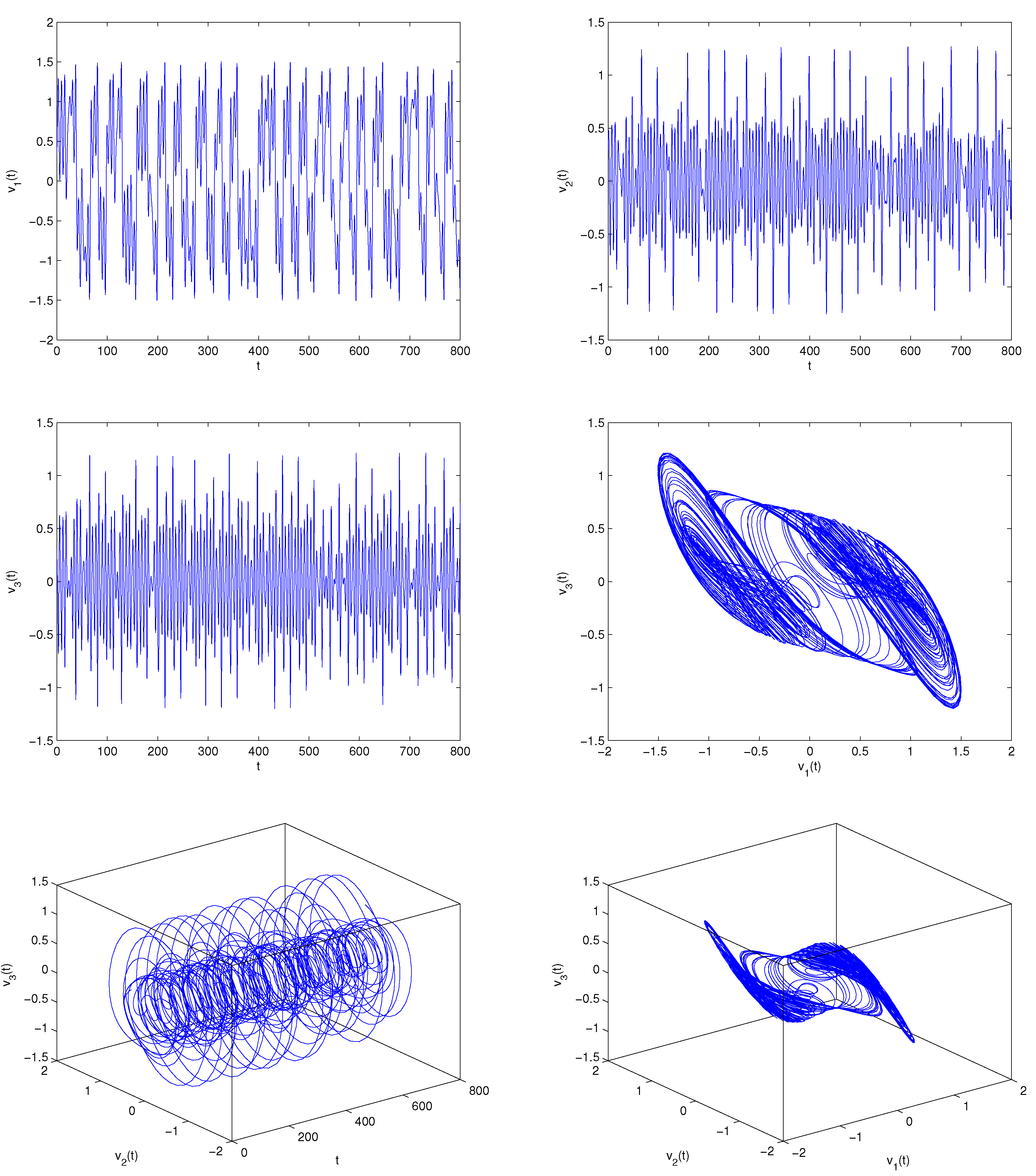
where . The investigation manifests that the fractional-order modificatory hybrid optical model (6) displays chaotic phenomenon under the parameter conditions The numerical simulation plots are presented in Figure 1.
In this current manuscript, we will explore two aspects as follows:
- (i)
- Taking advantage of a delayed feedback controller to eliminate chaos in model (6) and explore the stability and generation of Hopf bifurcation of a fractional-order controlled modificatory hybrid optical model.
- (ii)
- Making use of a suitable mixed controller including state feedback and parameter perturbation to suppress chaos in model (6) and investigate the stability and generation of Hopf bifurcation of a fractional-order controlled modificatory hybrid optical model.
The primary contribution of this manuscript is stated as follows:
- A proper delayed feedback controller is effectively devised to control the chaotic phenomenon of model (6).
- A proper mixed controller including state feedback and parameter perturbation is resoundingly designed to suppress the chaotic phenomenon of model (6).
- The exploration way can also be utilized to probe into the chaos control of lots of other fractional-order dynamical models.
The fabric of this manuscript is as follows. Some requisite knowledge on the fractional-order differential system is prepared in Section 2. In Section 3, the chaotic phenomenon of model (6) is controlled by using a suitable delayed feedback controller. In Section 4, the chaotic phenomenon of model (6) is controlled by virtue of a proper mixed controller including state feedback and parameter perturbation. In Section 5, computer simulations are put into effect to verify the established assertions. Section 6 completes this manuscript.
2. Preliminaries
In this part, we present some requisite definitions and lemmas on fractional-order differential system.
Definition 1
([41]). The Riemann–Liouville fractional integral of order ρ of the function is defined as follows:
where and .
Definition 2
([41]). The Caputo fractional-order derivative of order ρ of the function is defined as follows:
where and ι represents a positive integer (. In particular, if , then
Lemma 1
([42]). Consider the following fractional-order model: where Denote the root of the characteristic equation of , then the equilibrium point of model is locally asymptotically stable if and the equilibrium point of model is stable if and every critical eigenvalue which obeys owns geometric multiplicity one.
3. Chaos Suppression via Delayed Feedback Controller
In this part, we are to apply an appropriate delayed feedback controller to eliminate the chaotic phenomenon of the fractional-order modificatory hybrid optical model (6). Obeying the way of Yu and Chen [43], we propose the following delayed feedback controller:
where stands for feedback gain coefficient and denotes a delay. Adding the delayed feedback controller (7) to the first equation of model (6), we obtain
Obviously, model (8) has three equilibrium points . In this manuscript, we merely consider the equilibrium point For another two equilibrium points , we can deal with them in a similar way. Here, we omit it. The linear system of (8) around the equilibrium point is given by
The characteristic equation of (9) can be expressed as
Then
where
where
Assume that then (11) has the following form:
Assume that
is fulfilled, then all the roots of Equation (14) satisfy , and . Using Lemma 1, one can easily know that the equilibrium point of model (8) is locally asymptotically stable when .
Denote
If
is fulfilled, notice that , then Equation (21) owns at least one positive real root. Thus, Equation (11) owns at least one pair of purely roots. In view of Sun et al. [44], the following assertion can be built.
Lemma 2.
Let . Assume that
where
Lemma 3.
Let be the root of (11) at obeying , then
Making use of Lemma 1, the following assertion is easily built.
Theorem 1.
4. Chaos Suppression via Delayed Mixed Controller
In this part, we will apply a suitable delayed mixed controller which includes state feedback and parameter perturbation to control the chaos of the fractional-order modificatory hybrid optical model (6). Following the idea of [45,46], we obtain the following fractional-order controlled modificatory hybrid optical model
where are feedback gain parameters. Clearly, model (29) has the same equilibrium points as those in model (6). In this manuscript, we merely consider the equilibrium point For another two equilibrium points , we can deal with them in a similar way. Here, we omit it. The linear system of (29) near the equilibrium point reads
The characteristic equation of (30) takes the following form:
Then
where
where
If then (32) becomes
If
holds, then all the roots of (35) satisfy and . By virtue of Lemma 1, one obtains that the equilibrium point of model (29) is locally asymptotically stable when .
We assume that Equation (41) has six roots (say . Then, by
where Set In this case, we assume that Equation (41) has the root .
Next, the following assumption is presented.
where
Lemma 4.
Suppose that is the root of (32) at satisfying , , then
Using Lemma 1, we obtain the following result.
Theorem 2.
5. Examples
Example 1.
Consider the following fractional-order controlled modificatory hybrid optical model:
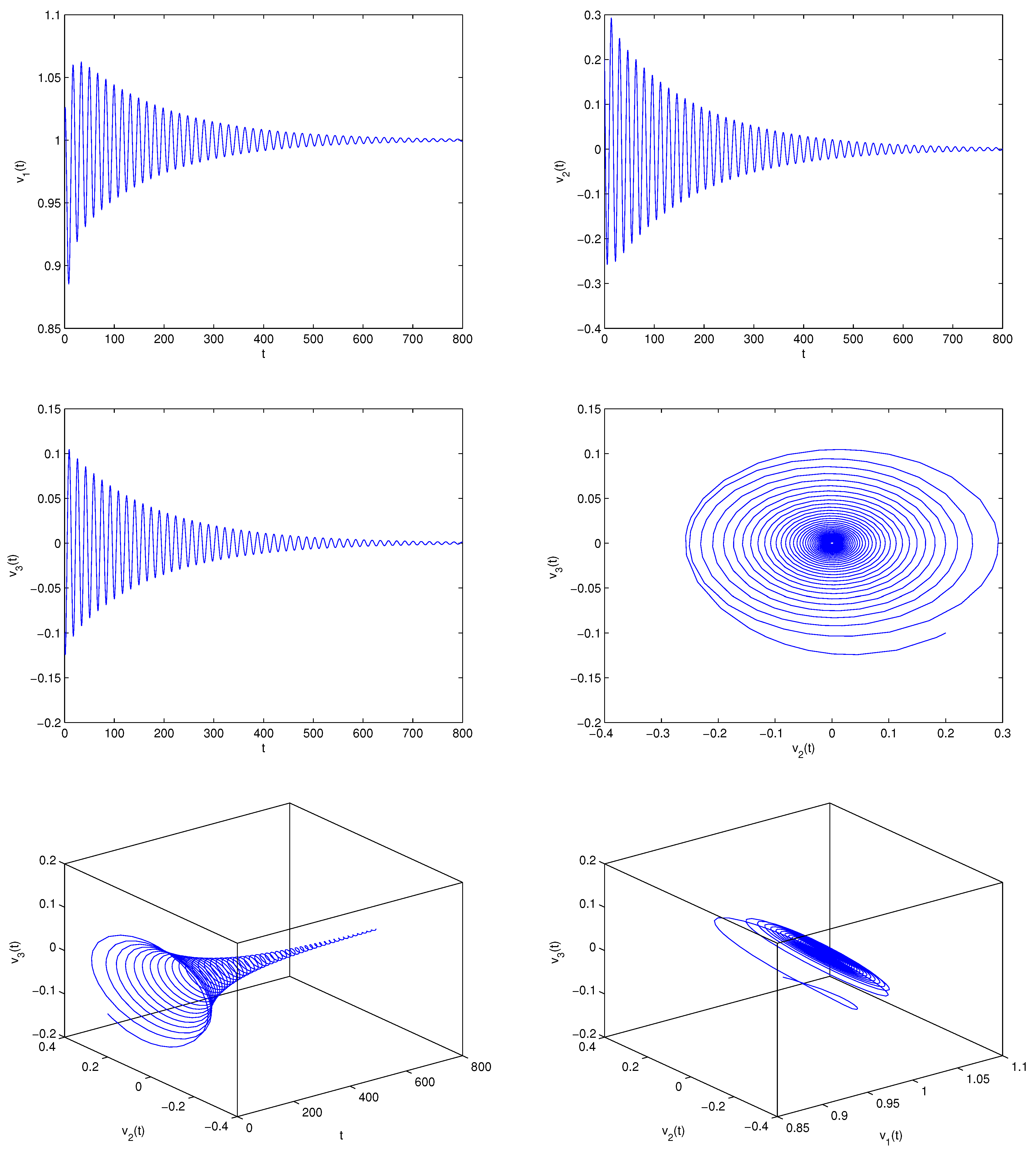
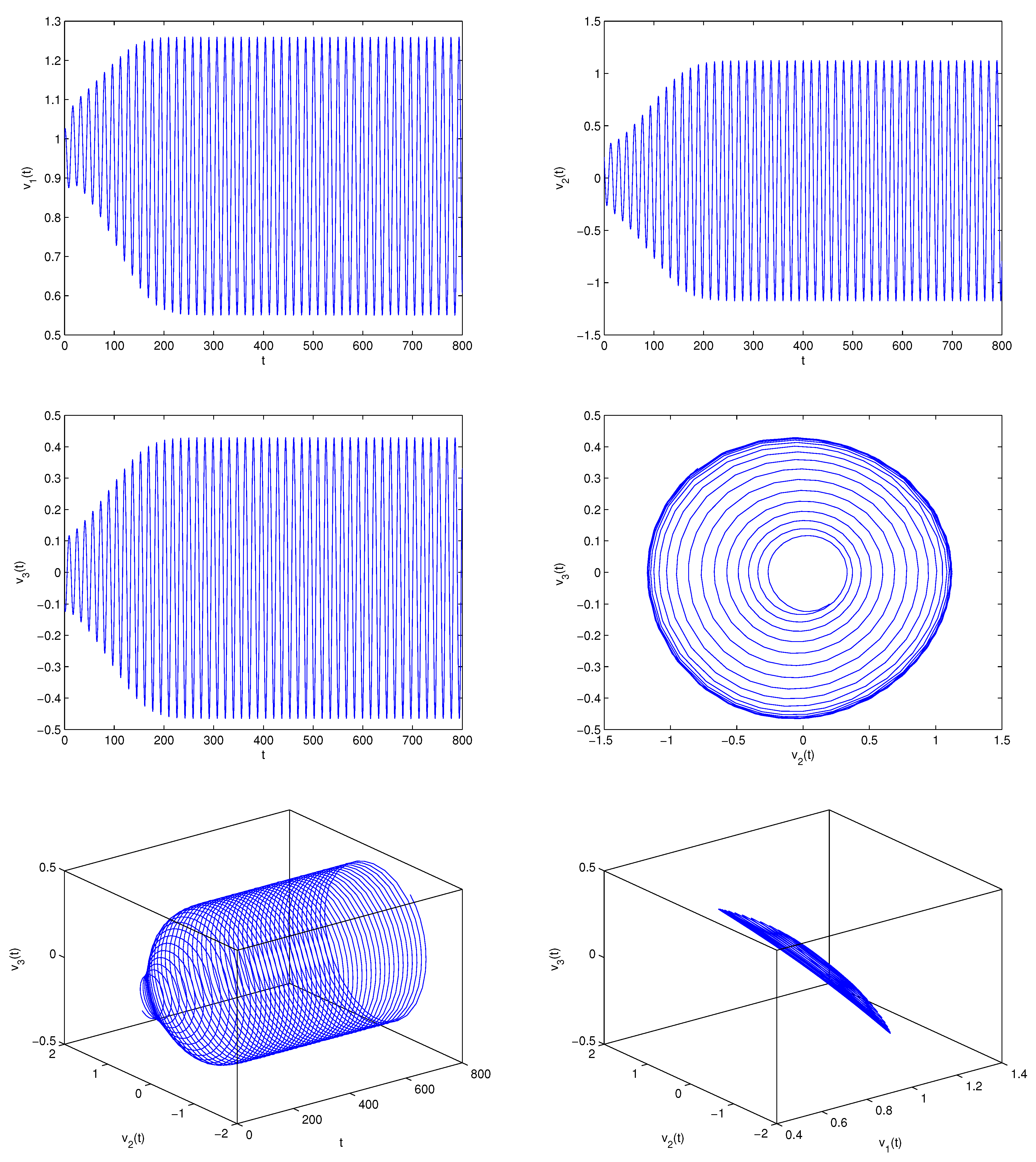
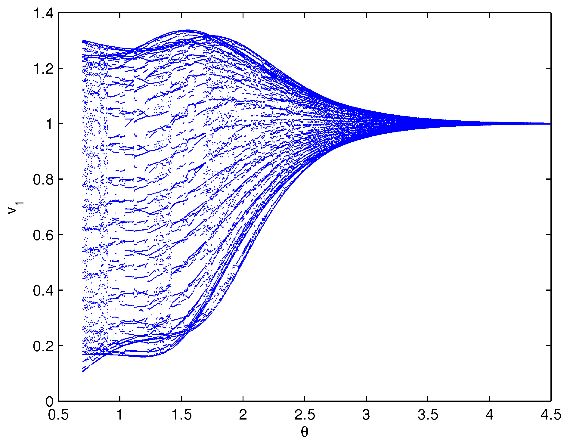
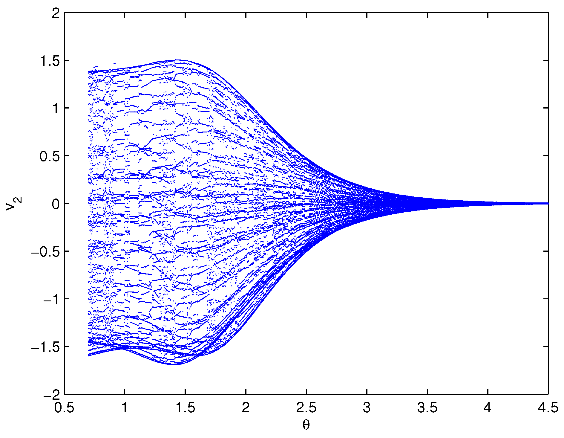
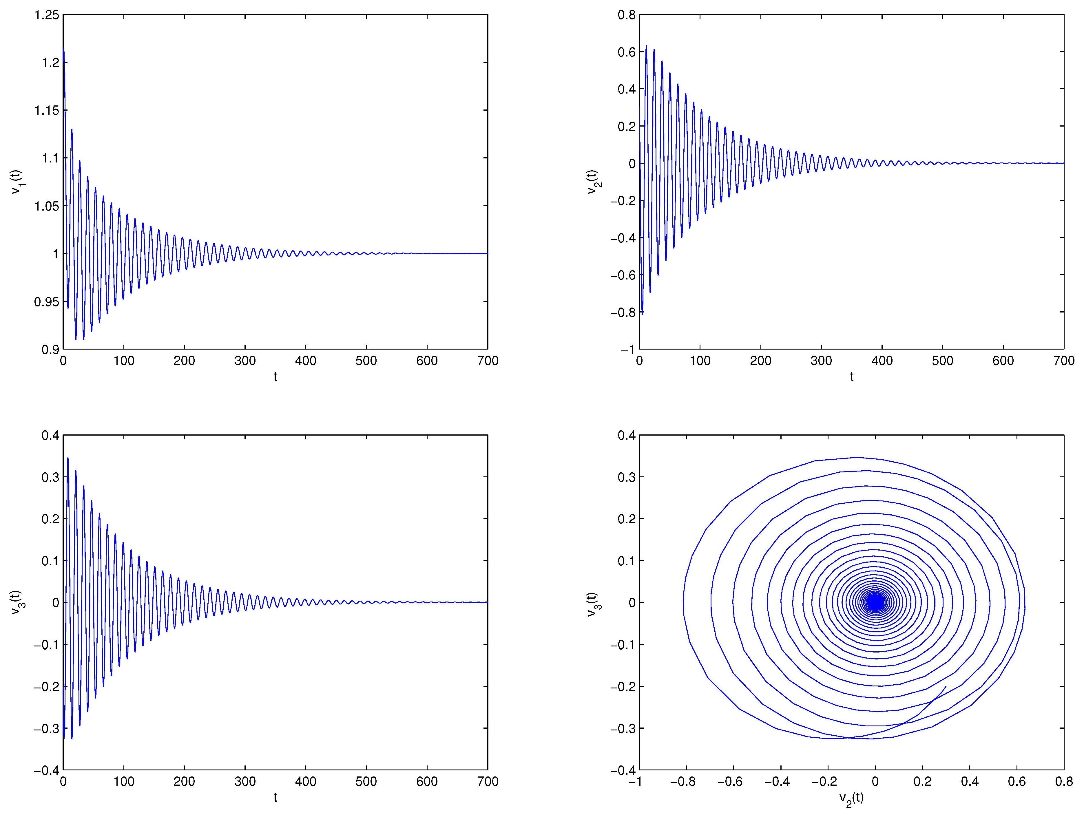
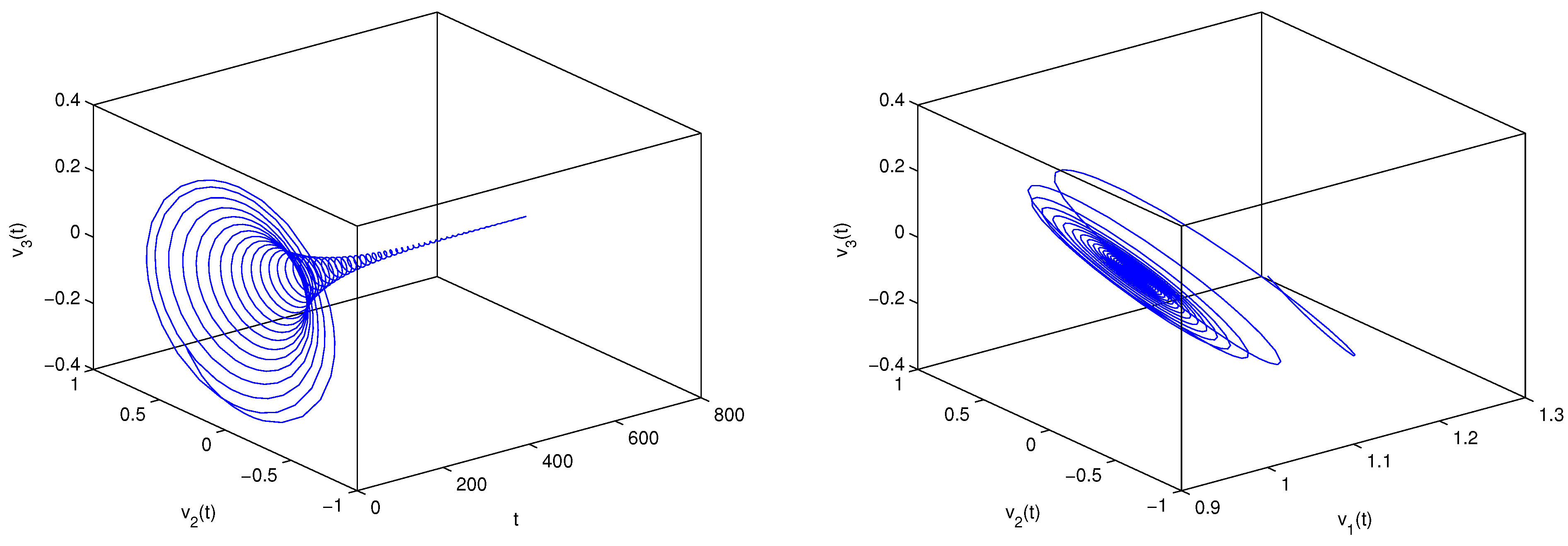
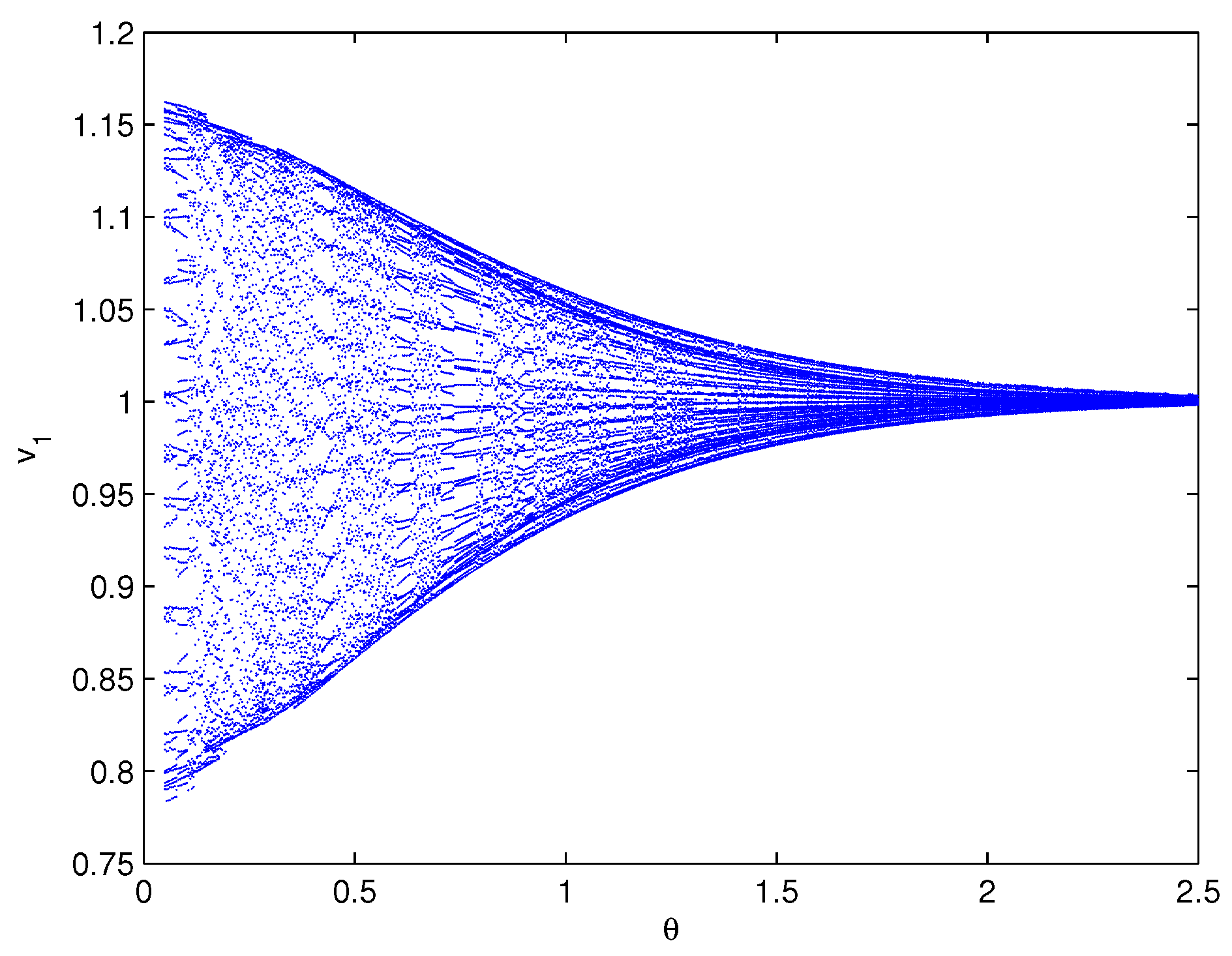
One can easily know that model (48) owns three equilibrium points . In this numerical simulation, we only focus on the equilibrium point Making use of the computer, one can determine . The assumptions – of Theorem 1 hold true. Select , which shows that falls into the interval range . The homologous numerical simulation plots are presented in Figure 2. It follows from Figure 2 that the three state variables will get close to , respectively, as Select , which indicates that passes through the critical delay value . The homologous numerical simulation plots are provided in Figure 3. It follows from Figure 3 that the three state variables will maintain a periodic vibratory level near , respectively, as Two situations clearly manifest the vanishing of the chaos of fractional-order chaotic modificatory hybrid optical model (6). Additionally, the bifurcation plots are given in Figure 4, Figure 5 and Figure 6 to manifest that the bifurcation value (with respect to the delay ) of model (48) is about . The simulation results powerfully illustrate the scientificity of the designed delayed feedback controller in this manuscript.
Example 2.
Consider the following fractional-order controlled modificatory hybrid optical model:
One can easily know that model (49) owns three equilibrium points . In this numerical simulation, we only focus on the equilibrium point Let Making use of the computer, one can determine . The assumptions and of Theorem 2 hold true. Select , which shows that falls into the interval range . The homologous numerical simulation plots are presented in Figure 7. It follows from Figure 7 that the three state variables will get close to , respectively, as Select , which indicates that passes through the critical delay value . The homologous numerical simulation plots are provided in Figure 8. It follows from Figure 8 that the three state variables will maintain a periodic vibratory level near , respectively, as Two situations clearly manifest the vanishing of the chaos of fractional-order chaotic modificatory hybrid optical model (6). Additionally, the bifurcation plots are given in Figure 9, Figure 10 and Figure 11 to manifest that the bifurcation value (with respect to the delay ) of model (49) is about . The simulation results powerfully illustrate the scientificity of the designed mixed controller in this manuscript.
Remark 3.
It follows from the computer simulation results of Examples 1 and 2, one can easily know that the stability domain of fractional-order controlled modificatory hybrid optical model (48) is enlarged and the time of occurrence of Hopf bifurcation of model (48) is postponed. (In controlled model (48), , but in controlled model (49), ).
6. Conclusions
For a long time, chaos suppression, which is an old and classic topic, has attracted great attention from many scholars in engineering circles. During the past several decades, plenty of chaos control techniques were proposed and very rich results have been achieved. In this present manuscript, we deal with the chaos suppression of a (FOMHO model) by virtue of two different control controllers. Taking advantage of an apposite delayed feedback controller, we effectively suppress the chaos of the (FOMHO model). A sufficient condition ensuring the stability and occurrence of Hopf bifurcation of the fractional-order controlled modificatory hybrid optical model is set up. By virtue of a proper delayed mixed controller that consists of state feedback and parameter perturbation, we successfully eliminate the chaotic behavior of the (FOMHO model). A sufficient condition which guarantees the stability and occurrence of Hopf bifurcation of the fractional-order controlled modificatory hybrid optical model is built. The exploration shows that the delay in the two controllers has a vital effect on the chaotic behavior. The acquired results of this manuscript are perfectly new, and the exploration idea of this manuscript can also be utilized to inquire into numerous chaos control aspects of fractional-order dynamical models in plentiful fields.
Author Contributions
Conceptualization, P.L. and C.X.; methodology, C.X.; software, R.G.; validation, P.L., R.G. and Y.L.; formal analysis, P.L.; investigation, Y.L; resources, R.G.; data curation, Y.L.; writing—original draft preparation, C.X.; writing—review and editing, C.X.; visualization, P.L.; supervision, P.L.; project administration, Y.L.; funding acquisition, C.X. All authors have read and agreed to the published version of the manuscript.
Funding
This work is supported by the National Natural Science Foundation of China (No. 62062018), the Project of High-level Innovative Talents of Guizhou Province ([2016]5651), the Guizhou Key Laboratory of Big Data Statistical Analysis ( No. [2019]5103), the basic research projects of key scientific research projects in Henan province (No. 20ZX001), the Key Science and Technology Research Project of Henan Province of China (Grant No. 222102210053), and the Key Scientific Research Project in Colleges and Universities of Henan Province of China (Grant No. 21A510003). The authors would like to thank the referees and the editor for helpful suggestions incorporated into this paper.
Data Availability Statement
No data were used to support this study.
Conflicts of Interest
The authors declare no conflict of interest.
References
- Zhou, L.Q.; Chen, F.Q. Chaos of the Rayleigh-Duffing oscillator with a non-smooth periodic perturbation and harmonic excitation. Math. Comput. Simul. 2022, 192, 1–18. [Google Scholar] [CrossRef]
- Akhtar, S.; Ahmed, R.; Batool, M.; Shah, N.A.; Chung, J.D. Stability, bifurcation and chaos control of a discretized Leslie prey-predator model. Chaos Solitons Fractals 2021, 152, 111345. [Google Scholar] [CrossRef]
- Adéchinan, A.J.; Kpomahou, Y.J.F.; Hinvi, L.A.; Miwadinou, C.H. Chaos, coexisting attractors and chaos control in a nonlinear dissipative chemical oscillator. Chin. J. Phys. 2022, 77, 2684–2697. [Google Scholar] [CrossRef]
- Ngounou, A.M.; Feulefack, S.C.M.; Tabejieu, L.M.A.; Nbendjo, B.R.N. Design, analysis and horseshoes chaos control on tension leg platform system with fractional nonlinear viscoelastic tendon force under regular sea wave excitation. Chaos Solitons Fractals 2022, 157, 111952. [Google Scholar] [CrossRef]
- Pietrych, L.; Sandubete, J.E.; Escot, L. Solving the chaos model-data paradox in the cryptocurrency market. Commun. Nonlinear Sci. Numer. Simul. 2021, 102, 105901. [Google Scholar] [CrossRef]
- Wojtusiak, A.M.; Balanov, A.G.; Savel’ev, S.E. Intermittent and metastable chaos in a memristive artificial neuron with inertia. Chaos Solitons Fractals 2021, 142, 110383. [Google Scholar] [CrossRef]
- Ma, C.; Wang, X.Y. Hopf bifurcation and topological horseshoe of a novel finance chaotic system. Commun. Nonlinear Sci. Numer. Simul. 2012, 17, 721–730. [Google Scholar] [CrossRef]
- Abdelouahab, M.S.; Hamri, N. A new chaotic attractor from hybrid optical bistable system. Nonlinear Dyn. 2012, 67, 457–463. [Google Scholar] [CrossRef]
- Aqeel, M.; Azam, A.; Ayub, J. Control of chaos in krause and roberts geomagnetic chaotic system. Chin. J. Phys. 2022, 77, 1331–1341. [Google Scholar] [CrossRef]
- Kaur, R.P.; Sharma, A.; Sharma, A.K.; Sahu, G.P. Chaos control of chaotic plankton dynamics in the presence of additional food, seasonality, and time delay. Chaos Solitons Fractals 2021, 153, 111521. [Google Scholar] [CrossRef]
- Li, Z.B.; Lu, W.; Gao, L.F.; Zhang, J.S. Nonlinear state feedback control of chaos system of brushless DC motor. Procedia Comput. Sci. 2021, 183, 636–640. [Google Scholar] [CrossRef]
- Yin, X.; She, J.H.; Liu, Z.T.; Wu, M.; Kaynak, O. Chaos suppression in speed control for permanent-magnet-synchronous-motor drive system. J. Frankl. Inst. 2020, 357, 13283–13303. [Google Scholar] [CrossRef]
- Ott, E.; Grebogi, C.; Yorke, J.A. Controlling chaos. Phys. Rev. Lett. 1990, 64, 1196–1199. [Google Scholar] [CrossRef]
- Du, J.G.; Huang, T.W.; Sheng, Z.H.; Zhang, H.B. A new method to control chaos in an economic system. Appl. Math. Comput. 2010, 217, 2370–2380. [Google Scholar] [CrossRef]
- Zheng, J.L. A simple universal adaptive feedback controller for chaos and hyperchaos control. Comput. Math. Appl. 2011, 61, 2000–2004. [Google Scholar] [CrossRef] [Green Version]
- Han, Y.Y.; Ding, J.P.; Du, L.; Lei, Y.M. Control and anti-control of chaos based on the moving largest Lyapunov exponent using reinforcement learning. Phys. D Nonlinear Phenom. 2021, 428, 133068. [Google Scholar] [CrossRef]
- Din, Q. Dynamics and chaos control for a novel model incorporating plant quality index and larch budmoth interaction. Chaos Solitons Fractals 2021, 153, 111595. [Google Scholar] [CrossRef]
- Shi, J.P.; He, K.; Fang, H. Chaos, Hopf bifurcation and control of a fractional-order delay financial system. Math. Comput. Simul. 2022, 194, 348–364. [Google Scholar] [CrossRef]
- Eshaghi, S.; Ghaziani, R.K.; Ansari, A. Hopf bifurcation, chaos control and synchronization of a chaotic fractional-order system with chaos entanglement function. Math. Comput. Simul. 2020, 172, 321–340. [Google Scholar] [CrossRef]
- Xu, C.J.; Zhang, W.; Aouiti, C.; Liu, Z.X.; Liao, M.X.; Li, P.L. Further investigation on bifurcation and their control of fractional-order BAM neural networks involving four neurons and multiple delays. Math. Methods Appl. Sci. 2021. [Google Scholar] [CrossRef]
- Huang, C.D.; Liu, H.; Chen, X.P.; Cao, J.D.; Alsaedi, A. Extended feedback and simulation strategies for a delayed fractional-order control system. Phys. A Stat. Mech. Its Appl. 2020, 545, 123127. [Google Scholar] [CrossRef]
- Mitschke, F.; Flüggen, N. Chaotic behavior of a hybrid optical bistable system without time delay. Appl. Phys. 1984, 35, 59–64. [Google Scholar] [CrossRef]
- Das, M.; Samanta, G.P. A delayed fractional-order food chain model with fear effect and prey refuge. Math. Comput. Simul. 2020, 178, 218–245. [Google Scholar] [CrossRef]
- Xu, C.J.; Zhang, W.; Aouiti, C.; Liu, Z.X.; Yao, L.Y. Further analysis on dynamical properties of fractional-order bi-directional associative memory neural networks involving double delays. Math. Methods Appl. Sci. 2022. [Google Scholar] [CrossRef]
- Tan, H.L.; Wu, J.W.; Bao, H.B. Event-triggered impulsive synchronization of fractional-order coupled neural networks. Appl. Math. Comput. 2022, 429, 127244. [Google Scholar] [CrossRef]
- Xiao, M.; Zheng, W.X.; Lin, J.X.; Jiang, G.P.; Zhao, L.D.; Cao, J.D. Fractional-order PD control at Hopf bifurcations in delayed fractional-order small-world networks. J. Frankl. Inst. 2017, 354, 7643–7667. [Google Scholar] [CrossRef]
- Zhang, Z.; Wang, Y.N.; Zhang, J.; Ai, Z.Y.; Liu, F. Novel stability results of multivariable fractional-order system with time delay. Chaos Solitons Fractals 2022, 157, 111943. [Google Scholar] [CrossRef]
- Huang, C.D.; Wang, J.; Chen, X.P.; Cao, J.D. Bifurcations in a fractional-order BAM neural network with four different delays. Neural Netw. 2021, 141, 344–354. [Google Scholar] [CrossRef]
- Xu, C.J.; Liao, M.X.; Li, P.L.; Yuan, S. Impact of leakage delay on bifurcation in fractional-order complex-valued neural networks. Chaos Solitons Fractals 2021, 142, 110535. [Google Scholar] [CrossRef]
- Xu, C.J.; Liao, M.X.; Li, P.L.; Guo, Y.; Liu, Z.X. Bifurcation properties for fractional order delayed BAM neural networks. Cogn. Comput. 2021, 13, 322–356. [Google Scholar] [CrossRef]
- Li, N.; Yan, M.T. Bifurcation control of a delayed fractional-order prey-predator model with cannibalism and disease. Phys. A Stati. Mech. Appl. 2020, 600, 127600. [Google Scholar] [CrossRef]
- Barman, D.; Roy, J.; Alam, S. Modelling hiding behaviour in a predator-prey system by both integer order and fractional order derivatives. Ecol. Inform. 2022, 67, 101483. [Google Scholar] [CrossRef]
- Kaslik, E.; Rădulescu, I.R. Stability and bifurcations in fractional-order gene regulatory networks. Appl. Math. Comput. 2022, 421, 126916. [Google Scholar] [CrossRef]
- Yuan, J.; Zhao, L.Z.; Huang, C.D.; Xiao, M. Stability and bifurcation analysis of a fractional predator-prey model involving two nonidentical delays. Math. Comput. Simul. 2021, 181, 562–580. [Google Scholar] [CrossRef]
- Xue, G.M.; Lin, F.N.; Li, S.G.; Liu, H. Adaptive fuzzy finite-time backstepping control of fractional-order nonlinear systems with actuator faults via command-filtering and sliding mode technique. Inf. Sci. 2022, 600, 189–208. [Google Scholar] [CrossRef]
- Djilali, S.; Ghanbari, B.; Bentout, S.; Mezouaghi, A. Turing-Hopf bifurcation in a diffusive mussel-algae model with time-fractional-order derivative. Chaos Solitons Fractals 2020, 138, 109954. [Google Scholar] [CrossRef]
- Borah, M.; Das, D.; Gayan, A.; Fenton, F.; Cherry, E. Control and anticontrol of chaos in fractional-order models of Diabetes, HIV, Dengue, Migraine, Parkinson’s and Ebola virus diseases. Chaos Solitons Fractals 2021, 153, 111419. [Google Scholar] [CrossRef]
- Akinlar, M.A.; Tchier, F.; Inc, M. Chaos control and solutions of fractional-order Malkus waterwheel model. Chaos Solitons Fractals 2020, 135, 109746. [Google Scholar] [CrossRef]
- Ouannas, A.; Khennaoui, A.A.; Grassi, G.; Bendoukha, S. On chaos in the fractional-order Grassi-Miller map and its control. J. Comput. Appl. Math. 2019, 358, 293–305. [Google Scholar] [CrossRef]
- Srivastava, M.; Agrawal, S.K.; Vishal, K.; Das, S. Chaos control of fractional order Rabinovich-Fabrikant system and synchronization between chaotic and chaos controlled fractional order Rabinovich-Fabrikant system. Appl. Math. Model. 2014, 38, 3361–3372. [Google Scholar] [CrossRef]
- Podlubny, I. Fractional Differential Equations; Academic Press: New York, NY, USA, 1999. [Google Scholar]
- Matignon, D. Stability results for fractional differential equations with applications to control processing. In Proceedings of the Computational Engineering in Systems and Application Multi-Conference, IMACS, Lille, France, 9–12 July 1996; pp. 963–968. [Google Scholar]
- Yu, P.; Chen, G.R. Hopf bifurcation control using nonlinear feedback with polynomial functions. Int. J. Bifurc. Chaos 2004, 14, 1683–1704. [Google Scholar] [CrossRef]
- Sun, Q.S.; Xiao, M.; Tao, B.B. Local bifurcation analysis of a fractional-order dynamic model of genetic regulatory networks with delays. Neural Process. Lett. 2018, 47, 1285–1296. [Google Scholar] [CrossRef]
- Zhang, Z.Z.; Yang, H.Z. Hybrid control of Hopf bifurcation in a two prey one predator system with time delay. In Proceedings of the 33rd Chinese Control Conference, Nanjing, China, 28–30 July 2014; pp. 6895–6900. [Google Scholar]
- Zhang, L.P.; Wang, H.N.; Xu, M. Hybrid control of bifurcation in a predator-prey system with three delays. Acta Phys. Sin. 2011, 60, 010506. [Google Scholar] [CrossRef]
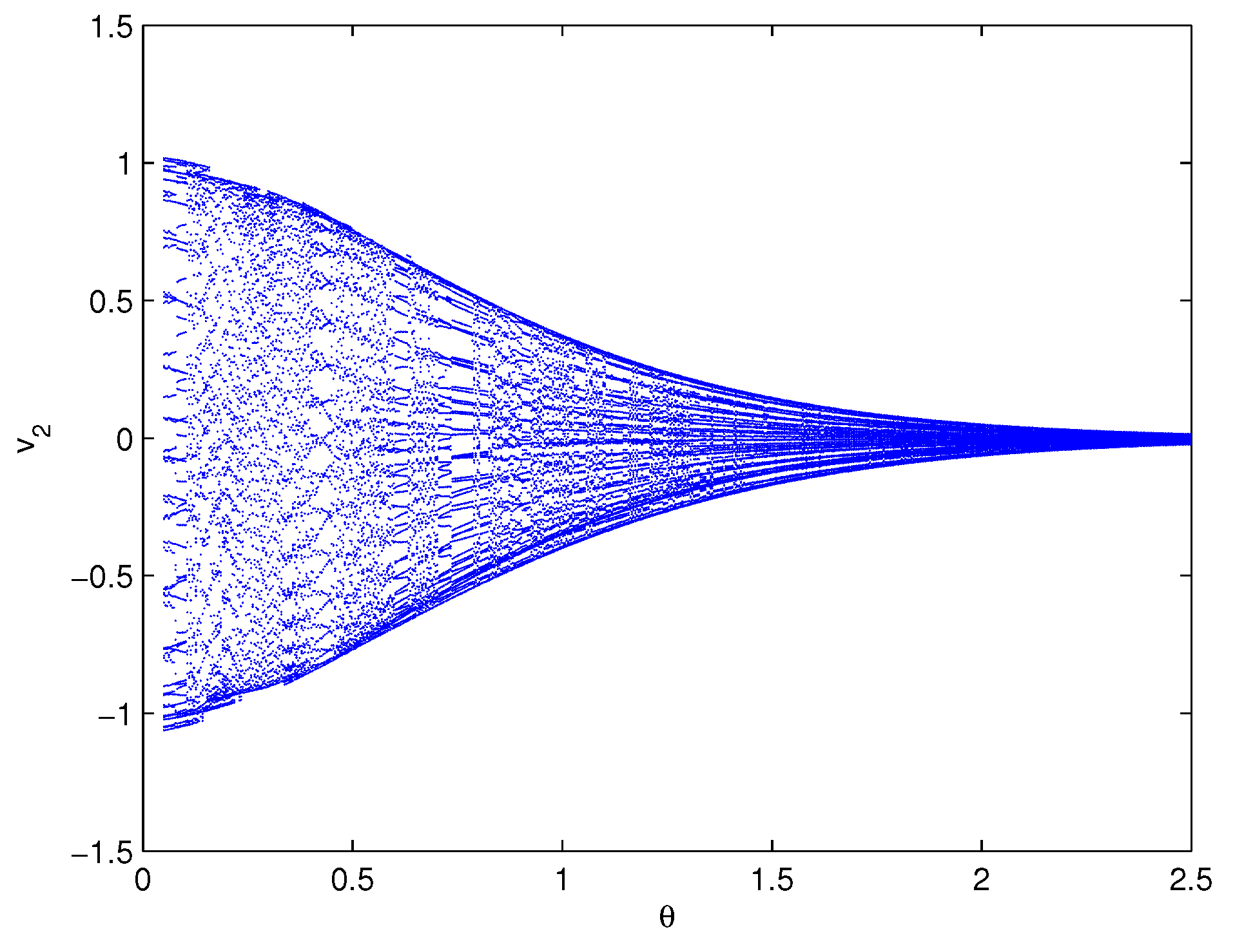
Figure 1.
Computer simulation results of model (6) involving the parameters It shows that model (6) displays a chaotic phenomenon.

Figure 2.
Numerical simulation results of the fractional-order controlled modificatory hybrid optical model (48) under the delay condition . The equilibrium point is locally asymptotically stable.
Figure 2.
Numerical simulation results of the fractional-order controlled modificatory hybrid optical model (48) under the delay condition . The equilibrium point is locally asymptotically stable.

Figure 3.
Numerical simulation results of the fractional-order controlled modificatory hybrid optical model (48) under the delay condition . Model (48) displays the Hopf bifurcation phenomenon near the equilibrium point .

Figure 4.
The bifurcation plot of the fractional-order controlled modificatory hybrid optical model (48): the time t versus the state variable .
Figure 4.
The bifurcation plot of the fractional-order controlled modificatory hybrid optical model (48): the time t versus the state variable .

Figure 5.
The bifurcation plot of the fractional-order controlled modificatory hybrid optical model (48): the time t versus the state variable .
Figure 5.
The bifurcation plot of the fractional-order controlled modificatory hybrid optical model (48): the time t versus the state variable .

Figure 6.
The bifurcation plot of the fractional-order controlled modificatory hybrid optical model (48): the time t versus the state variable .
Figure 6.
The bifurcation plot of the fractional-order controlled modificatory hybrid optical model (48): the time t versus the state variable .

Figure 7.
Numerical simulation results of the fractional-order controlled modificatory hybrid optical model (49) under the delay condition . The equilibrium point is locally asymptotically stable.
Figure 7.
Numerical simulation results of the fractional-order controlled modificatory hybrid optical model (49) under the delay condition . The equilibrium point is locally asymptotically stable.


Figure 8.
Numerical simulation results of the fractional-order controlled modificatory hybrid optical model (49) under the delay condition . Model (49) displays the Hopf bifurcation phenomenon near the equilibrium point .


Figure 9.
The bifurcation plot of the fractional-order controlled modificatory hybrid optical model (49): the time t versus the state variable .
Figure 9.
The bifurcation plot of the fractional-order controlled modificatory hybrid optical model (49): the time t versus the state variable .

Figure 10.
The bifurcation plot of the fractional-order controlled modificatory hybrid optical model (49): the time t versus the state variable .
Figure 10.
The bifurcation plot of the fractional-order controlled modificatory hybrid optical model (49): the time t versus the state variable .

Figure 11.
The bifurcation plot of the fractional-order controlled modificatory hybrid optical model (49): the time t versus the state variable .
Figure 11.
The bifurcation plot of the fractional-order controlled modificatory hybrid optical model (49): the time t versus the state variable .

Publisher’s Note: MDPI stays neutral with regard to jurisdictional claims in published maps and institutional affiliations. |
© 2022 by the authors. Licensee MDPI, Basel, Switzerland. This article is an open access article distributed under the terms and conditions of the Creative Commons Attribution (CC BY) license (https://creativecommons.org/licenses/by/4.0/).
Share and Cite
MDPI and ACS Style
Li, P.; Gao, R.; Xu, C.; Li, Y. Chaos Suppression of a Fractional-Order Modificatory Hybrid Optical Model via Two Different Control Techniques. Fractal Fract. 2022, 6, 359. https://0-doi-org.brum.beds.ac.uk/10.3390/fractalfract6070359
AMA Style
Li P, Gao R, Xu C, Li Y. Chaos Suppression of a Fractional-Order Modificatory Hybrid Optical Model via Two Different Control Techniques. Fractal and Fractional. 2022; 6(7):359. https://0-doi-org.brum.beds.ac.uk/10.3390/fractalfract6070359
Chicago/Turabian StyleLi, Peiluan, Rong Gao, Changjin Xu, and Ying Li. 2022. "Chaos Suppression of a Fractional-Order Modificatory Hybrid Optical Model via Two Different Control Techniques" Fractal and Fractional 6, no. 7: 359. https://0-doi-org.brum.beds.ac.uk/10.3390/fractalfract6070359