Modeling and Numerical Simulation for Covering the Fractional COVID-19 Model Using Spectral Collocation-Optimization Algorithm

Abstract

A primary aim of this study is to examine and simulate a fractional Coronavirus disease model by providing an efficient method for solving numerically this important model. In the Liouville-Caputo sense, the examined model consists of five fractional-order differential equations. With the Vieta-Lucas spectral collocation method, the unknown functions can be discretized and fractional derivatives can be obtained. With the system of nonlinear algebraic equations obtained, we can simplify the examined problem. In this system, the unknown coefficients are discovered by constructing and solving it as a restricted optimization problem. Some theoretical investigations are stated to examine the convergence analysis and stability analysis of the proposed approach and model. The results produced using the fractional finite difference technique (FDM), where the fractional differentiation operator was discretized using the Grünwald-Letnikov approach, are compared. The FDM relies heavily upon accurately turning the proposed model into a system of algebraic equations. To assess the algorithm’s correctness and usefulness, a numerical simulation is included.

1. Introduction

Coronavirus infection is one of the most well-known infections nowadays (COVID-19) [1]. This pandemic sickness, which was designated by the World Health Organization (WHO) on March 11, compelled large and small countries to take preventative steps in order to save the lives of its inhabitants and residents. The global economy has suffered as a result of the spread of this pandemic sickness. Companies, colleges, markets, and a variety of other institutions have adopted unusual precautionary steps as a result of this widely spread pandemic sickness. Travel within and outside of the countries has been halted for several months, and curfews have been implemented to reduce crowding and hence disease spread, according to [2]. The danger of this pandemic comes from its incredible ability to spread and the various types of infection that humans can contract.

Mathematical modeling plays an important role in our life [3,4,5]. Mathematical models are crucial not only in the forecast of disease outbreaks, but also in the prevention and treatment of disease outbreaks, according to [6]. One of the most important uses for modeling is to research infectious illnesses and how to develop effective control techniques. Depending on the assumptions made about transmission methods, there are a variety of models. For example, susceptible-infected-susceptible (SIS) systems have been used to model nonlinear occurrence rates and double pandemic theories [7], SIR (susceptible-infected-recovered) models have been used to consider whether or not an individual is aware of the existence of a disease [8], and many other models [9,10,11]. Researchers have been using and constructing mathematical models to gain insight into the pandemic’s mode of spread, propagation, effect, prevention, and control, as well as the effects of preventive measures like handwashing with disinfection and using hand sanitizer, since the debut of COVID-19 [12,13,14,15,16].

In reality, we cannot examine infectious disease dynamical systems using standard derivatives and integrals. Ordinal operators (derivatives and integrals) are not suited when the situation is unexpected, such as in the case of COVID-19, due to uncertainties related to the pandemic. Fractional-order models are more appropriate and accurate than integer-order models because they are more consistent with real-world challenges [17,18].

Finding a novel fractional derivative with non-singular kernels is critical, according to some writers, to address the demand for mathematical modeling of numerous real-world situations in various sectors of daily life [19,20]. Also, the role of these new operators are appearing in many applications like engineering, chemistry, electricity, and many other applications [21,22]. Because fractional differential equations (FDEs) rarely have a precise solution, they are frequently studied using approximate techniques [23,24,25]. The fractional order will be studied in this article in the Liouville-Caputo meaning (LC).

Definition 1.

The fractional derivative $D^{\alpha }$ of order α in the sense of Liouville-Caputo of a function $\phi \left(t\right)$ is defined as [26]:

$$D^{\alpha }\phi \left(t\right)=\frac{1}{\mathrm{\Gamma }(m-\alpha )}{\int }_0^t\frac{{\phi }^{(m-1)}\left(\tau \right)}{{(t-\tau )}^{\alpha -m+1}}d\tau ,t>0,m-1<\alpha \le m,m\in \mathbb{N}.$$

Following are a few properties of the LC-fractional derivative operator [20].

For some constants $c_i$, $i=0,1,\cdots ,n,$ we have:

$$D^{\alpha }\left(\sum _{i=0}^n{c}_i{\psi }_i\left(t\right)\right)=\sum _{i=0}^n{c}_i{D}^{\alpha }{\psi }_i\left(t\right),$$

(1)

and

$$D^{\alpha }{t}^n=\frac{\mathrm{\Gamma }(n+1)}{\mathrm{\Gamma }(n+1-\alpha )}{t}^{n-\alpha },n>\alpha -1.$$

(2)

Definition 2.

The shifted Grünwald-Letnikov fractional derivative is defined as [20]:

$$\frac{d^{\alpha }\phi \left(t\right)}{d{t}^{\alpha }}=\underset{h⟶0}{lim}\frac{1}{h^{\alpha }}\sum _{i=0}^{\left[\frac{t}{h}\right]+1}{(-1)}^i\left(\begin{array}{c}\alpha \\ i\end{array}\right)\phi (t-(i-1)h),h\in \mathbb{R}\mathrm{is}\mathrm{a}\mathrm{constant}.$$

(3)

Lemma 1. ([27]) Assume that ρ a constant, if $\mid t\mid <\rho$ and $\rho \phi \left(t\right)$ can be expressed in terms of a power series. Then

$$D_R^{\alpha }\phi \left(\tau \right)=\frac{1}{h^{\alpha }}{\mathrm{\Delta }}_h^{\alpha }\phi \left(nh\right)+O\left(h\right),(h⟶0),$$

(4)

for $0<\alpha <\rho$ and a series of step size h, $\frac{\tau }{h}\in \mathbb{N}$, where $D_R^{\alpha }$ is the RL fractional derivative; and

$${\mathrm{\Delta }}_h^{\alpha }\phi \left(nh\right)=\sum _{i=0}^n{(-1)}^i\left(\begin{array}{c}\alpha \\ i\end{array}\right)\phi \left(t_{n-i}\right).$$

In the instance of LC sense, we can find the following by considering the relation between both definitions [27] for $0<\alpha \le 1$:

$$D^{\alpha }\phi \left(\tau \right)=\frac{1}{h^{\alpha }}{\mathrm{\Delta }}_h^{\alpha }\phi \left(nh\right)-\frac{{\tau }^{-\alpha }}{\mathrm{\Gamma }(1-\alpha )}\phi \left(0\right)+O\left(h\right),(h⟶0).$$

(5)

For more properties, and theoretical results [19,20].

Many researchers have presented a variety of numerical techniques to study and simulate the behavior of solutions for differential equations, including the finite difference method [25], the finite volume method [28], spectral methods [29], and many others [22,30]. One of the most effective techniques for simulating FDEs is the spectral approaches. The most well-known virtue of these techniques are their capacity to produce reliable results with very low degrees of freedom error [31]. Some polynomials, such as Vieta-Lucas polynomials, have an orthogonality property that can be utilized to estimate functions on the interval $[a,b]$. These polynomials play a crucial part in the FDEs [31] techniques. The Vieta-Lucas spectral collocation approach was used in this research to discretize the unknown functions and fractional derivatives of the proposed model’s solution, and the model under consideration was turned into a simple system of nonlinear algebraic equations using the method.

The fundamental goal of this study, as well as its originality, is to expand the COVID-19 system to a fractional-order model. The numerical solution for the suggested model is derived utilizing the spectral collocation approach to attain this goal. The unknown coefficients of the series-solution are discovered by constructing and solving the obtained nonlinear system of algebraic equations as a restricted optimization problem, substantially simplifying it to find these coefficients and the solution. We also compare the suggested method via fractional FDM to the Grünwald-Letnikov approach. The qualitative analysis of the model is examined. Finally, we present comparison research. We emphasize the study’s fundamental weakness, which is the lack of real data, thus we examine the model from a theoretical standpoint using its equivalent system of ODEs. The manuscript is structured as following: Section 2 contains preliminaries and some concepts concerning the model formulation and proves the nonnegative solutions, equilibrium points, and the stability of the model; in addition it defines some concepts about the introduced polynomials. Section 3 presents an approximate of the LC-derivative and the convergence analysis. Section 4 gives numerical implementation the proposed methods, where we implement the proposed method, and the fractional FDM. In addition, numerical simulation is given in Section 5. Finally, in Section 6, we give the conclusion as well as future work that is planned.

2. Preliminaries and Some Concepts

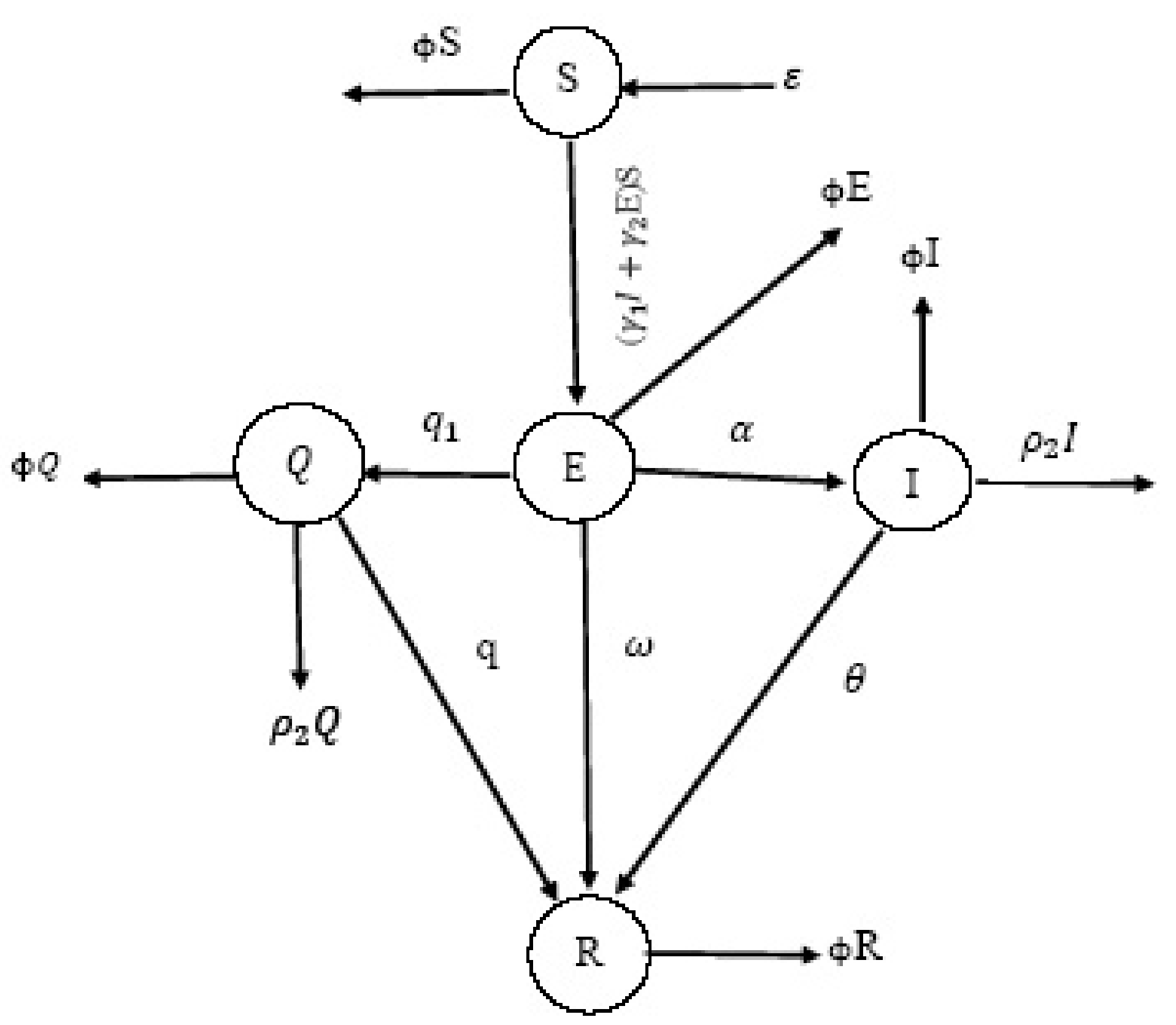
2.1. General Notes and Formulation the Fractional COVID-19 Model

Based on the natural death rate of susceptible individuals $\varphi$, a constant increase $ϵ$ in the susceptible population is maintained. People’s susceptibility will decrease at constant rates ${\gamma }_1$ and ${\gamma }_2$ as they come in contact with exposed or infected individuals, leading to a greater number of exposed individuals. As individuals exposed to COVID-19 become infected, $\theta +\varphi +{\rho }_1$ decreases and increases; in this formula, $\theta$ represents a patient’s recovery rate from exposure to COVID-19, and ${\rho }_1$ represents the mortality rate of individuals infected with it. Likewise, as a percentage of recovered individuals die due to natural causes, the number of exposed, infected, and quarantined individuals declines, and others [32,33]. Furthermore, the number of individuals quarantined in relation to the total number of individuals exposed increases by $q_1$ and decreases at rate $(\mathrm{\Lambda }+\varphi +{\rho }_2)Q$, whereas q is the recovery rate from quarantine to recovery and ${\rho }_2$ is the death rate of quarantined individuals.

Consider the following classifications in this population:

• $N\left(t\right)$: the whole human population,
• $S\left(t\right)$: Susceptible individuals,
• $E\left(t\right)$: Exposed individuals,
• $I\left(t\right)$: Infected individuals,
• $Q\left(t\right)$: Quarantined persons,
• $R\left(t\right)$: Those who have recovered/removed themselves from COVID-19.

As a result of these considerations, the following nonlinear system of FDEs is proposed as a mathematical model to characterize COVID-19 propagation dynamics ($\forall t\ge 0$):

$$\begin{array}{c}{D}^{\nu }S\left(t\right)=ϵ-\left({\gamma }_{1}I\left(t\right)+{\gamma }_{2}E\left(t\right)\right)S\left(t\right)-\varphi S\left(t\right),\hfill \\ D^{\nu }E\left(t\right)=\left({\gamma }_{1}I\left(t\right)+{\gamma }_{2}E\left(t\right)\right)S\left(t\right)-\left(q_1+\omega +\alpha +\varphi \right)E\left(t\right),\hfill \\ D^{\nu }I\left(t\right)=\alpha E\left(t\right)-\left(\theta +\varphi +{\rho }_1\right)I\left(t\right),\hfill \\ D^{\nu }Q\left(t\right)=q_{1}E\left(t\right)-\left(\mathrm{\Lambda }+\varphi +{\rho }_2\right)Q\left(t\right),\hfill \\ D^{\nu }R\left(t\right)=\omega E\left(t\right)+\theta I\left(t\right)+\mathrm{\Lambda }Q\left(t\right)-\varphi R\left(t\right).\hfill \end{array}$$

(6)

The SEIQR model’s employed coefficients (parameters) are defined as follows and Figure 1 [34]: ${\gamma }_1$ and ${\gamma }_2$ are contact rates of susceptible individuals with infected individuals and susceptible individuals with exposed individuals, respectively; $q_1$ and $q_2$ are the quarantined rates of exposed individuals and infected individuals, respectively; $\mathrm{\Lambda }$, $\omega$ and $\theta$ are the recovery rates of quarantine to recovered, exposed individuals due to immunity during the latent period, and of exposed individuals due to immunity, respectively; ${\rho }_2$ and ${\rho }_1$ are the death rates caused by COVID-19 in confined individuals and infected individuals, respectively; $\alpha$ represent the rate at which people who have been exposed to the virus get infected following a latent period; $ϵ$ and $\varphi$ represent the recruitment rate of individuals and the natural death rate of individuals, respectively.

The total population is $N\left(t\right)=S\left(t\right)+E\left(t\right)+I\left(t\right)+Q\left(t\right)+R\left(t\right)$. Let $S_0,E_0,I_0,Q_0$ and $R_0$ reflect the original sizes of the subpopulations vulnerable, exposed, infected, quarantined, and recovered. In addition, the following requirements are met:

$$S\left(0\right)=S_0,E\left(0\right)=E_0,I\left(0\right)=I_0,Q\left(0\right)=Q_0,R\left(0\right)=R_0.$$

Using this model (6) in its fractional version, we may more clearly assess the impact of the COVID-19 pandemic’s transmission in the future and in past, thanks to the memory effect of fractional derivatives. While mathematical models with integer derivatives are crucial for understanding the dynamics of epidemiological systems, they have certain limits because these systems lack memory or non-local effects, and hence these models in their current state are not always appropriate. As a result, in order to effectively examine various natural phenoms, it is important to convert several epidemiological models into FDEs. FDEs are extensively used in the study of unusual events in nature and the theory of complex systems in general, and they take into account the curve’s characteristics to a large extent. Finally, it can explain temporal delays, fractal features, and other phenomena.

The following two cases are considered [34] to derive and compute the reproductive number ${\mathfrak{R}}_0$:

(1)

In the absence of COVID-19, the system ${\xi }_0=\left(S_{\ast }^0,E_{\ast }^0,I_{\ast }^0,Q_{\ast }^0,R_{\ast }^0\right)=(\alpha /\varphi ,0,0,0,0)$ as equilibrium point.

(2)

Otherwise, the equilibrium assumes the form ${\xi }_1=\left(S_{\ast }^1,E_{\ast }^1,I_{\ast }^1,Q_{\ast }^1,R_{\ast }^1\right)$, where

$$S_{\ast }^1=\frac{\left(q_1+\omega +\alpha +\varphi \right)\left(\theta +\varphi +{\rho }_1\right)}{{\gamma }_1\alpha +{\gamma }_2\left(\theta +\varphi +{\rho }_1\right)},E_{\ast }^1=\frac{\left(ϵ-\varphi S_{\ast }^1\right)\left(\theta +\varphi +{\rho }_1\right)}{\left[{\gamma }_1\alpha +{\gamma }_2\left(\theta +\varphi +{\rho }_1\right)\right]S_{\ast }^1},$$

$$I_{\ast }^1=\frac{\alpha E_{\ast }^1}{\theta +\varphi +{\rho }_1},Q_{\ast }^1=\frac{q_1{E}_{\ast }^1}{\mathrm{\Lambda }+\varphi +{\rho }_2},R_{\ast }^1=\frac{\omega E_{\ast }^1+\theta I_{\ast }^1+\mathrm{\Lambda }{Q}_{\ast }^1}{\varphi }.$$

The Jacobian matrix of the system (6) in the cases of ${\xi }_0$ and ${\xi }_1$ are, respectively [34]:

$$F=\left(\begin{array}{cccc}\frac{{\gamma }_2ϵ}{\varphi }& \frac{{\gamma }_1ϵ}{\varphi }& 0& 0\\ 0& 0& 0& 0\\ 0& 0& 0& 0\\ 0& 0& 0& 0\end{array}\right),V=\left(\begin{array}{cccc}\omega +\alpha +\varphi +q_1& 0& 0& 0\\ -\alpha & \theta +\varphi +{\rho }_1& 0& 0\\ -q_1& 0& \mathrm{\Lambda }+\varphi +{\rho }_2& 0\\ -\omega & -\theta & -\mathrm{\Lambda }& \varphi \end{array}\right).$$

The basic reproductive number is calculated by ${\mathfrak{R}}_0=\rho \left(F{V}^{-1}\right)$ and is defined as the average number of secondary infections created when one sick individual is introduced into a group of susceptible people [34], where $\rho$ stands for the spectral radius of the generation matrix $F{V}^{-1}$ of the model structure (6) and take the following formula [35]:

$${\mathfrak{R}}_0=\frac{ϵ\left[{\gamma }_2\left(\theta +\varphi +{\rho }_1\right)+{\gamma }_1\alpha \right]}{\left(\omega +\alpha +\varphi +q_1\right)\left(\theta +\varphi +{\rho }_1\right)}.$$

(7)

2.2. Nonnegative Solutions, Stability and Equilibrium Points

Assume that $R_{+}^5=\{X\in R^5:X\ge 0\}$ and $X\left(t\right)={(x_1\left(t\right),x_2\left(t\right),x_3\left(t\right),x_4\left(t\right),x_5\left(t\right))}^T$, and for $0<\nu \le 1$, let $f\left(x\right),D^{\nu }f\left(x\right)\in C[a,b]$, then from the generalized mean value theorem (GMVT) [36], we have [37]:

$$f\left(x\right)=f\left(a\right)+\frac{1}{\mathrm{\Gamma }\left(\nu \right)}{D}^{\nu }f\left(\delta \right){(x-a)}^{\nu },\mathrm{with}0\le \delta \le x,\forall x\in [a,b].$$

In view of GMVT, if $D^{\nu }f\left(x\right)\ge 0,\forall x\in (0,b)$ then $f\left(x\right)$ is increasing ∀$x\in [0,b]$  and if $D^{\nu }f\left(x\right)\le 0,\forall x\in (0,b)$ then $f\left(x\right)$ is decreasing ∀$x\in [0,b]$.

Theorem 1

([38]). ${(S\left(t\right),E\left(t\right),I\left(t\right),Q\left(t\right),R\left(t\right))}^T$ a unique solution of (6) and remains in $R_{+}^5$.

Theorem 2

([39,40]). For the following fractional nonlinear dynamical system:

$$D^{\nu }{x}_i\left(t\right)=f_i(x_1,x_2,x_3,x_4,x_5),i=1,2,3,4,5,0<\nu \le 1,$$

(8)

with $x_1\left(0\right)=x_{10},x_2\left(0\right)=x_{20},x_3\left(0\right)=x_{30},x_4\left(0\right)=x_{40},x_5\left(0\right)=x_{50},$ the equilibrium point ${\chi }^{\ast }=(x_1^{\ast },x_2^{\ast },x_3^{\ast },x_4^{\ast },x_5^{\ast })$ is locally asymptotically stable if the Matignon’s conditions [40] given by:

$$|\arg \left({\lambda }_i\right)|>\frac{\pi }{2}\nu ,i=1,2,3,4,5,$$

are satisfied, where ${\lambda }_i$ are the eigen-values of the Jacobian matrix J evaluated at the equilibrium point ${\chi }^{\ast }$. The equilibrium points are obtained by setting the right hand sides of the model system (6) to zero, i.e.,

$$D^{\nu }S\left(t\right)=0,D^{\nu }E\left(t\right)=0,D^{\nu }I\left(t\right)=0,D^{\nu }Q\left(t\right)=0,D^{\nu }R\left(t\right)=0,$$

as a result, we have the following system of algebraic equations:

$$\begin{array}{cc}\hfill & ϵ-\left({\gamma }_{1}I\left(t\right)+{\gamma }_{2}E\left(t\right)\right)S\left(t\right)-\varphi S\left(t\right)=0,\hfill \\ & \left({\gamma }_{1}I\left(t\right)+{\gamma }_{2}E\left(t\right)\right)S\left(t\right)-\left(q_1+\omega +\alpha +\varphi \right)E\left(t\right)=0,\hfill \\ & \alpha E\left(t\right)-\left(\theta +\varphi +{\rho }_1\right)I\left(t\right)=0,\hfill \\ & q_{1}E\left(t\right)-\left(\mathrm{\Lambda }+\varphi +{\rho }_2\right)Q\left(t\right)=0,\hfill \\ & \omega E\left(t\right)+\theta I\left(t\right)+\mathrm{\Lambda }Q\left(t\right)-\varphi R\left(t\right)=0.\hfill \end{array}$$

(9)

If $I=0$ the system (9) has a disease-free equilibrium point ${\xi }_0=\left(\frac{ϵ}{\varphi },0,0,0,0\right)$. The Jacobian matrix $J\left({\xi }_0\right)$ for the system given in (9) evaluated at the disease-free equilibrium point ${\xi }_0$ as:

$$J\left({\xi }_0\right)=\left(\begin{array}{ccccc}-\varphi & -\frac{{\gamma }_2ϵ}{\varphi }& -\frac{{\gamma }_1ϵ}{\varphi }& 0& 0\\ 0& \frac{{\gamma }_2ϵ}{\varphi }-(q_1+\omega +\alpha +\varphi )& \frac{{\gamma }_1ϵ}{\varphi }& 0& 0\\ 0& \alpha & -(\theta +\varphi +{\rho }_1)& 0& 0\\ 0& q_1& 0& (\mathrm{\Lambda }+\varphi +{\rho }_2)& 0\\ 0& \omega & \theta & \mathrm{\Lambda }& -\varphi \end{array}\right).$$

Theorem 3.

If ${\mathfrak{R}}_0<1$, then ${\xi }_0=(S_{\ast }^0,E_{\ast }^0,I_{\ast }^0,Q_{\ast }^0,R_{\ast }^0)$ is locally asymptotically stable.

Theorem 4.

The endemic equilibrium point ${\xi }_1=(S_{\ast }^1,E_{\ast }^1,I_{\ast }^1,Q_{\ast }^1,R_{\ast }^1)$ of the system given by (9) is locally asymptotically stable iff ${\mathfrak{R}}_0>1$.

The proof of the two Theorems 3 and 4 can be done in details as in [39].

Theorem 5.

• The equilibrium point ${\xi }_0$ is globally asymptotically stable iff ${\mathfrak{R}}_0<1$.
• If ${\mathfrak{R}}_0>1$, then ${\xi }_1$ is globally asymptotically stable, and it is unstable otherwise.

Parameterizations of the model (6) are based on literature values and the least curve fitting method is employed to fit or estimate parameters given the data from Wuhan, China, between 21–28 January. The real data is available starting from 21 January 2020, and extending to 28 January 2020 [41], see

Table 1. Fitted and estimated parameter values [41] for (6).

Parameter	Value	Source
$ϵ$	0.5	Estimated
$q_1$	0.001	Fitted
$\omega$	0.00398	Fitted
$\alpha$	0.085432	Fitted
$\varphi$	0.5	Estimated
$\theta$	0.09871	Fitted
${\rho }_1$	0.0047876	Fitted
${\rho }_2$	0.000001231	Fitted
$\mathrm{\Lambda }$	0.1243	Fitted
${\gamma }_1$	1.05	Fitted
${\gamma }_2$	$0.005\left({\xi }_0\right)$	Fitted
	$1.05\left({\xi }_1\right)$	Fitted

.

The goal is the development of a numerical scheme for numerically simulating and solving the coronavirus mathematical model, as well as making the necessary comparisons. By solving this model, we can predict the number of infected persons and the projected number of infections with this disease owing to infection spread, as well as the number of infections after recovery, which greatly aids in the health and economic management of this disease.

2.3. Shifted Vieta-Lucas Polynomials

In this subsection, we’re looking for a class of orthogonal polynomials which will be used to create a set of orthogonal polynomials called Vieta-Lucas polynomials on the interval $[-2,2]$ by using their recurrence relations and its analytical formula. The Vieta-Lucas polynomials; ${\mathrm{VL}}_m\left(z\right)$ of degree $m\in {\mathbb{N}}_0$ is defined by [31]:

$${\mathrm{VL}}_m\left(z\right)=2cos(marccos\left(0.5z\right)),-2\le z\le 2.$$

Using the transformation $z=4t-2$, we can generate a new class of orthogonal polynomials on the interval $[0,1]$, which are the shifted Vieta-Lucas polynomials (SVLPs), and it will be denoted by ${\mathrm{VL}}_m^s\left(t\right)$ and can be obtained as follows:

$${\mathrm{VL}}_m^s\left(t\right)={\mathrm{VL}}_m(4t-2).$$

It easy to see that  ${\mathrm{VL}}_0^{\ast }\left(t\right)=2,{\mathrm{VL}}_1^{\ast }\left(t\right)=4t-2.$ Also, we find ${\mathrm{VL}}_m^s\left(0\right)=2{(-1)}^m$ and ${\mathrm{VL}}_m^s\left(1\right)=2,m=0,1,2,\cdots .$

Let $v\left(t\right)\in L^2[0,1]$, then $v\left(t\right)$ can be written in terms of ${\mathrm{VL}}_m^s\left(t\right)$ as follows:

$$v\left(t\right)=\sum _{j=0}^{\infty }{\kappa }_j{\mathrm{VL}}_j^{\ast }\left(t\right),$$

(10)

where ${\kappa }_j$ are constants. By considering first the $m+1$ terms only of Equation (10), then

$$v_m\left(t\right)=\sum _{j=0}^m{\kappa }_j{\mathrm{VL}}_j^{\ast }\left(t\right),$$

(11)

where the coefficients ${\kappa }_j,j=0,2,\dots ,m$ can be estimated with the help of the orthogonal property of the SVLPs.

3. An Approximate of the LC-Derivative and the Convergence Analysis

This section will offer an approximate fractional derivative formula using SVLPs, as well as a convergence analysis using the proposed approximation’s error estimate.

Theorem 6.

The LC-fractional-order derivative can be approximated as [26]:

$$D^{\nu }\left(v_m\left(t\right)\right)=\sum _{j=\lceil \nu \rceil }^m\sum _{s=0}^{j-\lceil \nu \rceil }{\kappa }_j{\chi }_{j,s}^{\left(\nu \right)}{t}^{j-s-\nu },$$

(12)

where

$${\chi }_{j,s}^{\left(\nu \right)}={(-1)}^s\frac{4^{j-s}\left(2j\right)\mathrm{\Gamma }(2j-s)\mathrm{\Gamma }(j-s+1)}{\mathrm{\Gamma }(s+1)\mathrm{\Gamma }(2j-2s+1)\mathrm{\Gamma }(j-s+1-\nu )}.$$

Theorem 7.

Assume that $v\left(t\right)\in L^2[0,1]$ concerning the weight function in the orthogonality relation of ${\mathrm{VL}}_m^s\left(t\right)$ on $[0,1]$; $w\left(t\right)=\frac{1}{\sqrt{t-t^2}}$, and assume $v^{{}^{″}}\left(t\right)<\ell$. Then $v\left(t\right)$ can be approximated by $v_m\left(t\right)$ and written as a linear combination of $m+1$ terms only of ${\mathrm{VL}}_m^s\left(t\right)$, as in Equation (11). Also, this series converges uniformly to the function $v\left(t\right)$ as $m\to \infty$, and its coefficients are bounded, i.e.

$$\left|{\kappa }_j\right|\le \frac{\ell }{4j\left(j^2-1\right)},j>2.$$

In addition, in the case, $v\left(t\right)$ is an m-times continuously differentiable on $[0,1]$, then the norm of the error $(L_w^2[0,1]$-norm), and the absolute error bound are estimated by the following, respectively:

$${∥v\left(t\right)-v_m\left(t\right)∥}_w<\frac{\ell }{12\sqrt{m^3}}.$$

$$∥v\left(t\right)-v_m\left(t\right)∥\le \frac{\mathrm{\Delta }{\mathrm{\Omega }}^{m+1}}{(m+1)!}\sqrt{\pi },$$

where

$$\mathrm{\Delta }=\underset{t\in [0,1]}{max}{v}^{(m+1)}\left(t\right),\mathrm{and}\mathrm{\Omega }=max\left\{1-t_0,t_0\right\}.$$

4. Numerical Studies

4.1. Implementation of the Proposed Method

We will use the spectral collocation approach, which is based on the summation of SVLPs, to convert the system of ODEs that describes the proposed model (6) into an algebraic equations system The unknown coefficients in the sequence of solutions are obtained by optimizing this system as a restricted optimization problem. The VLSCOM is the name given to the coupling of two well-known approaches. The following steps will be used as algorithm to solve the given problem (6) numerically using this technique:

• The solution for the problem (6) can be expressed and approximated as a finite series of SVLPs, namely,

  $$\begin{array}{cc}\hfill S_m\left(t\right)& =\sum _{j=0}^m{a}_j{\mathrm{VL}}_j^{\ast }\left(t\right),E_m\left(t\right)=\sum _{j=0}^m{b}_j{\mathrm{VL}}_j^{\ast }\left(t\right),I_m\left(t\right)=\sum _{j=0}^m{c}_j{\mathrm{VL}}_j^{\ast }\left(t\right),\hfill \\ & Q_m\left(t\right)=\sum _{j=0}^m{d}_j{\mathrm{VL}}_j^{\ast }\left(t\right),R_m\left(t\right)=\sum _{j=0}^m{e}_j{\mathrm{VL}}_j^{\ast }\left(t\right).\hfill \end{array}$$

  (13)
• We substitute from (13) and (12) in (6) to obtain:

  $$\begin{array}{cc}\hfill \sum _{j=\lceil \nu \rceil }^m\sum _{s=0}^{j-\lceil \nu \rceil }& a_j{\chi }_{j,s}^{\left(\nu \right)}{t}^{j-s-\nu }=\hfill \\ & ϵ-\left(\varphi +{\gamma }_1\left(\sum _{j=0}^m{c}_j{\mathrm{VL}}_j^{\ast }\left(t\right)\right)+{\gamma }_2\left(\sum _{j=0}^m{b}_j{\mathrm{VL}}_j^{\ast }\left(t\right)\right)\right)\left(\sum _{j=0}^m{a}_j{\mathrm{VL}}_j^{\ast }\left(t\right)\right),\hfill \end{array}$$

  (14)

  $$\begin{array}{cc}\hfill \sum _{j=\lceil \nu \rceil }^m\sum _{s=0}^{j-\lceil \nu \rceil }{b}_j{\chi }_{j,s}^{\left(\nu \right)}{t}^{j-s-\nu }=& \left({\gamma }_1\left(\sum _{j=0}^m{c}_j{\mathrm{VL}}_j^{\ast }\left(t\right)\right)+{\gamma }_2\left(\sum _{j=0}^m{b}_j{\mathrm{VL}}_j^{\ast }\left(t\right)\right)\right)\left(\sum _{j=0}^m{a}_j{\mathrm{VL}}_j^{\ast }\left(t\right)\right)\hfill \\ & -\left(q_1+\omega +\alpha +\varphi \right)\left(\sum _{j=0}^m{b}_j{\mathrm{VL}}_j^{\ast }\left(t\right)\right),\hfill \end{array}$$

  (15)

  $$\begin{array}{cc}\hfill \sum _{j=\lceil \nu \rceil }^m& \sum _{s=0}^{j-\lceil \nu \rceil }{c}_j{\chi }_{j,s}^{\left(\nu \right)}{t}^{j-s-\nu }=\alpha \left(\sum _{j=0}^m{b}_j{\mathrm{VL}}_j^{\ast }\left(t\right)\right)-\left(\theta +\varphi +{\rho }_1\right)\left(\sum _{j=0}^m{c}_j{\mathrm{VL}}_j^{\ast }\left(t\right)\right),\hfill \end{array}$$

  (16)

  $$\begin{array}{cc}\hfill \sum _{j=\lceil \nu \rceil }^m& \sum _{s=0}^{j-\lceil \nu \rceil }{d}_j{\chi }_{j,s}^{\left(\nu \right)}{t}^{j-s-\nu }=q_1\left(\sum _{j=0}^m{b}_j{\mathrm{VL}}_j^{\ast }\left(t\right)\right)-\left(\mathrm{\Lambda }+\varphi +{\rho }_2\right)\left(\sum _{j=0}^m{d}_j{\mathrm{VL}}_j^{\ast }\left(t\right)\right),\hfill \end{array}$$

  (17)

  $$\begin{array}{cc}\hfill \sum _{j=\lceil \nu \rceil }^m\sum _{s=0}^{j-\lceil \nu \rceil }{e}_j{\chi }_{j,s}^{\left(\nu \right)}{t}^{j-s-\nu }=& \omega \left(\sum _{j=0}^m{b}_j{\mathrm{VL}}_j^{\ast }\left(t\right)\right)+\theta \left(\sum _{j=0}^m{c}_j{\mathrm{VL}}_j^{\ast }\left(t\right)\right)+\mathrm{\Lambda }\left(\sum _{j=0}^m{d}_j{\mathrm{VL}}_j^{\ast }\left(t\right)\right)\hfill \\ & -\varphi \left(\sum _{j=0}^m{e}_j{\mathrm{VL}}_j^{\ast }\left(t\right)\right).\hfill \end{array}$$

  (18)
• The corresponding initial conditions of the model (6) can be approximated as follows:

  $$\begin{array}{c}\sum _{j=0}^{m}2{(-1)}^j{a}_j=S_0,\sum _{j=0}^{m}2{(-1)}^j{b}_j=E_0,\sum _{j=0}^{m}2{(-1)}^j{c}_j=I_0,\hfill \\ \sum _{j=0}^{m}2{(-1)}^j{d}_j=Q_0,\sum _{j=0}^{m}2{(-1)}^j{e}_j=R_0.\hfill \end{array}$$

  (19)
• Then, (14)–(19) will be collocated at $m+1$ of nodes at $t_k,k=0,1,2,\cdots ,m$ to obtain a nonlinear system of $5(m+1)$ algebraic equations.
• The problem defined by (14)–(19) is expressed as a restricted optimization problem with the cost functions (CFs) as follows:

  $$\begin{array}{cc}\hfill CF1=& \sum _{k=0}^n|\sum _{j=\lceil \nu \rceil }^m\sum _{s=0}^{j-\lceil \nu \rceil }{a}_j{\chi }_{j,s}^{\left(\nu \right)}{t}_k^{j-s-\nu }-ϵ\hfill \\ & +\left(\varphi +{\gamma }_1\left(\sum _{j=0}^m{c}_j{\mathrm{VL}}_j^{\ast }\left(t_k\right)\right)+{\gamma }_2\left(\sum _{j=0}^m{b}_j{\mathrm{VL}}_j^{\ast }\left(t_k\right)\right)\right)\left(\sum _{j=0}^m{a}_j{\mathrm{VL}}_j^{\ast }\left(t_k\right)\right)|,\hfill \end{array}$$

  (20)

  $$\begin{array}{cc}\hfill CF2=& \sum _{k=0}^n|\sum _{j=\lceil \nu \rceil }^m\sum _{s=0}^{j-\lceil \nu \rceil }{b}_j{\chi }_{j,s}^{\left(\nu \right)}{t}_k^{j-s-\nu }-\left({\gamma }_1\left(\sum _{j=0}^m{c}_j{\mathrm{VL}}_j^{\ast }\left(t_k\right)\right)+{\gamma }_2\left(\sum _{j=0}^m{b}_j{\mathrm{VL}}_j^{\ast }\left(t_k\right)\right)\right).\hfill \\ & \left(\sum _{j=0}^m{a}_j{\mathrm{VL}}_j^{\ast }\left(t_k\right)\right)+\left(q_1+\omega +\alpha +\varphi \right)\left(\sum _{j=0}^m{b}_j{\mathrm{VL}}_j^{\ast }\left(t_k\right)\right)|,\hfill \end{array}$$

  (21)

  $$\begin{array}{cc}\hfill CF3=& \sum _{k=0}^n|\sum _{j=\lceil \nu \rceil }^m\sum _{s=0}^{j-\lceil \nu \rceil }{c}_j{\chi }_{j,s}^{\left(\nu \right)}{t}_k^{j-s-\nu }-\alpha \left(\sum _{j=0}^m{b}_j{\mathrm{VL}}_j^{\ast }\left(t_k\right)\right)+\left(\theta +\varphi +{\rho }_1\right)\left(\sum _{j=0}^m{c}_j{\mathrm{VL}}_j^{\ast }\left(t_k\right)\right)|,\hfill \end{array}$$

  (22)

  $$\begin{array}{cc}\hfill CF4=& \sum _{k=0}^n|\sum _{j=\lceil \nu \rceil }^m\sum _{s=0}^{j-\lceil \nu \rceil }{d}_j{\chi }_{j,s}^{\left(\nu \right)}{t}_k^{j-s-\nu }-q_1\left(\sum _{j=0}^m{b}_j{\mathrm{VL}}_j^{\ast }\left(t_k\right)\right)+\left(\mathrm{\Lambda }+\varphi +{\rho }_2\right)\left(\sum _{j=0}^m{d}_j{\mathrm{VL}}_j^{\ast }\left(t_k\right)\right)|,\hfill \end{array}$$

  (23)

  $$\begin{array}{cc}\hfill CF5=& \sum _{k=0}^n|\sum _{j=\lceil \nu \rceil }^m\sum _{s=0}^{j-\lceil \nu \rceil }{e}_j{\chi }_{j,s}^{\left(\nu \right)}{t}_k^{j-s-\nu }-\omega \left(\sum _{j=0}^m{b}_j{\mathrm{VL}}_j^{\ast }\left(t_k\right)\right)-\theta \left(\sum _{j=0}^m{c}_j{\mathrm{VL}}_j^{\ast }\left(t_k\right)\right)\hfill \\ & -\mathrm{\Lambda }\left(\sum _{j=0}^m{d}_j{\mathrm{VL}}_j^{\ast }\left(t_k\right)\right)+\varphi \left(\sum _{j=0}^m{e}_j{\mathrm{VL}}_j^{\ast }\left(t_k\right)\right)|,\hfill \end{array}$$

  (24)

  and the constraints (Cons)

  $$\begin{array}{cc}\hfill \mathrm{Cons}=& |\sum _{j=0}^{m}2{(-1)}^j{a}_j-S_0|+|\sum _{j=0}^{m}2{(-1)}^j{b}_j-E_0|+|\sum _{j=0}^{m}2{(-1)}^j{c}_j-I_0|\hfill \\ & +|\sum _{j=0}^{m}2{(-1)}^j{d}_j-Q_0|+|\sum _{j=0}^{m}2{(-1)}^j{e}_j-R_0|.\hfill \end{array}$$

  (25)
• For the unknowns $a_j,b_j,c_j,d_j,e_j,j=0,1,2,\cdots ,m$, we apply the Penalty Leap Frog approach [42] to solve the restricted optimization problem (20)–(25). Then, using the formula, we may construct an approximation solution (13).

The approach for the approximate solution is now summarized using the Algorithm 1.

Algorithm 1:

Expand in terms of ${\mathrm{VL}}_m^s\left(t\right)$ on the solution as a linear combination. Substitute this expansion and the presented approximate formula of the LC-derivatives to convert the given problem to a system of nonlinear algebraic equations. Collocate such a system by using appropriate collocation points. Express the resulting system as a cost-function-constrained optimization problem. Get the required coefficients by solving the resulting solution using the Penalty Leap Frog approach, and then get the approximate solution.

4.2. Implementation of the Fractional FDM

First, for system (6), we consider:

$$\begin{array}{cc}\hfill & D^{\nu }{S}_n\left(t\right)=ϵ-\left({\gamma }_1{I}_n\left(t\right)+{\gamma }_2{E}_n\left(t\right)\right)S_n\left(t\right)-\varphi S_n\left(t\right),\hfill \\ & D^{\nu }{E}_n\left(t\right)=\left({\gamma }_1{I}_n\left(t\right)+{\gamma }_2{E}_n\left(t\right)\right)S_n\left(t\right)-\left(q_1+\omega +\alpha +\varphi \right)E_n\left(t\right),\hfill \\ & D^{\nu }{I}_n\left(t\right)=\alpha E_n\left(t\right)-\left(\theta +\varphi +{\rho }_1\right)I_n\left(t\right),\hfill \\ & D^{\nu }{Q}_n\left(t\right)=q_1{E}_n\left(t\right)-\left(\mathrm{\Lambda }+\varphi +{\rho }_2\right)Q_n\left(t\right),\hfill \\ & D^{\nu }{R}_n\left(t\right)=\omega E_n\left(t\right)+\theta I_n\left(t\right)+\mathrm{\Lambda }{Q}_n\left(t\right)-\varphi R_n\left(t\right).\hfill \end{array}$$

(26)

Second, we use $t_n=nh$, where $n=0,1,\cdots ,M,Mh=T$ and the abbreviations $S_n,E_n,I_n,Q_n,$ and $R_n,$ for approximation of the true solutions $S\left(t_n\right),E\left(t_n\right),$$I\left(t_n\right),Q\left(t_n\right),$ and $R\left(t_n\right),$ in the grid point $t_n$.

By applying the Equations (5)–(26), we obtain:

$$\frac{1}{h^{\alpha }}\sum _{i=0}^{n+1}{(-1)}^i{\psi }_i^{\alpha }{S}_{n+1-i}-\frac{{\left(nh\right)}^{-\alpha }}{\mathrm{\Gamma }(1-\alpha )}{S}_0=ϵ-\left({\gamma }_1{I}_n\left(t\right)+{\gamma }_2{E}_n\left(t\right)\right)S_n\left(t\right)-\varphi S_n\left(t\right),$$

(27)

$$\frac{1}{h^{\alpha }}\sum _{i=0}^{n+1}{(-1)}^i{\psi }_i^{\alpha }{E}_{n+1-i}-\frac{{\left(nh\right)}^{-\alpha }}{\mathrm{\Gamma }(1-\alpha )}{E}_0=\left({\gamma }_1{I}_n\left(t\right)+{\gamma }_2{E}_n\left(t\right)\right)S_n\left(t\right)-\left(q_1+\omega +\alpha +\varphi \right)E_n\left(t\right),$$

(28)

$$\frac{1}{h^{\alpha }}\sum _{i=0}^{n+1}{(-1)}^i{\psi }_i^{\alpha }{I}_{n+1-i}-\frac{{\left(nh\right)}^{-\alpha }}{\mathrm{\Gamma }(1-\alpha )}{I}_0=\alpha E_n\left(t\right)-\left(\theta +\varphi +{\rho }_1\right)I_n\left(t\right),$$

(29)

$$\frac{1}{h^{\alpha }}\sum _{i=0}^{n+1}{(-1)}^i{\psi }_i^{\alpha }{Q}_{n+1-i}-\frac{{\left(nh\right)}^{-\alpha }}{\mathrm{\Gamma }(1-\alpha )}{Q}_0=q_1{E}_n\left(t\right)-\left(\mathrm{\Lambda }+\varphi +{\rho }_2\right)Q_n\left(t\right),$$

(30)

$$\frac{1}{h^{\alpha }}\sum _{i=0}^{n+1}{(-1)}^i{\psi }_i^{\alpha }{R}_{n+1-i}-\frac{{\left(nh\right)}^{-\alpha }}{\mathrm{\Gamma }(1-\alpha )}{R}_0=\omega E_n\left(t\right)+\theta I_n\left(t\right)+\mathrm{\Lambda }{Q}_n\left(t\right)-\varphi R_n\left(t\right),$$

(31)

where ${\psi }_i^{\alpha }=\left(\begin{array}{c}\alpha \\ i\end{array}\right)$.

5. Numerical Simulation

In this part of the work, we will present some numerical simulations for the studied model (6) with distinct values of $ϵ,{\gamma }_1,{\gamma }_2,\varphi ,q_1,\omega ,{\rho }_1,{\rho }_2,\alpha ,\theta ,\mathrm{\Lambda },$ and the initial conditions $S_0,E_0,I_0,Q_0,R_0.$ The numerical simulation for the analyzed model using the proposed technique is shown in Figure 2, Figure 3, Figure 4, Figure 5, Figure 6 and Figure 7 as following:

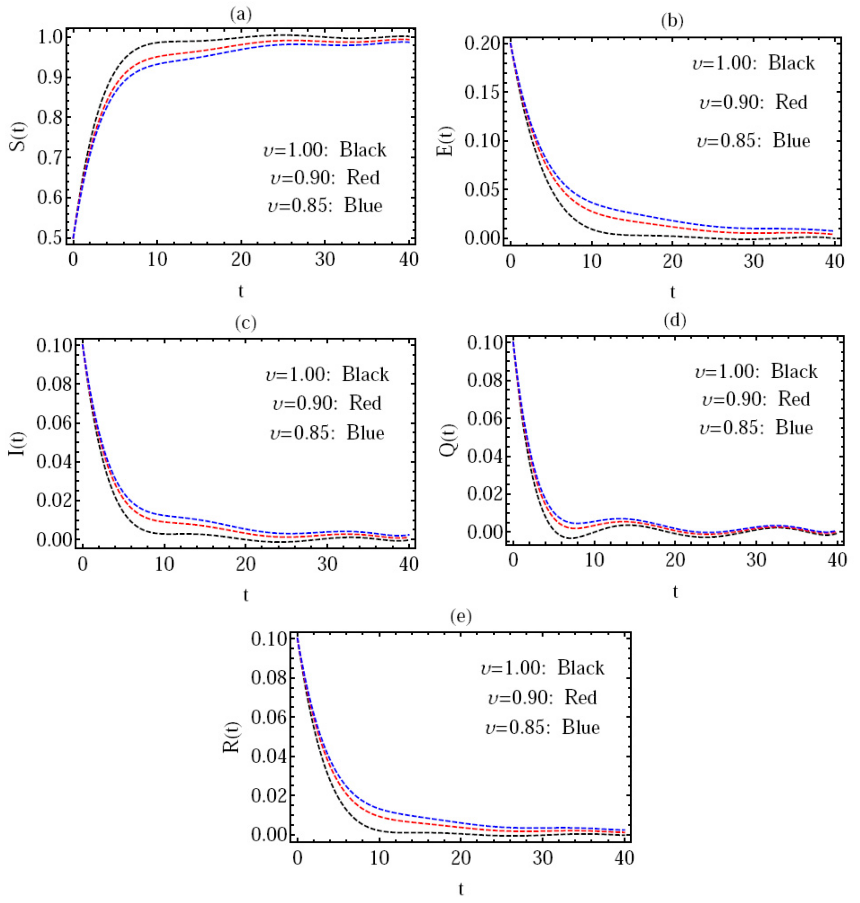
• Figure 2 depicts the behavior of the approximate solution for various values of $\nu =1.0,0.9,0.85;$ in ($0,40$) and $m=6$, with $S_0=0.5,E_0=0.2,I_0=Q_0=R_0=0.1$, and the parameters $ϵ=0.5,{\gamma }_1=1.05,{\gamma }_2=0.005,\varphi =0.5,q_1=0.001,\omega =0.00398,{\rho }_1=0.0047876,{\rho }_2=0.000001231,\alpha =0.085432,\theta =0.09871,\mathrm{\Lambda }=0.1243.$ Where in this case, ${\mathfrak{R}}_0=0.130112<1$, and we can also see that the disease-free equilibrium point ${\xi }_0$ is locally asymptotically stable, according to Theorem 3.
  Because the recovered population expands substantially, we can see and confirm that the majority of the population will recover from the COVID-19 dynamics in this image (see Figure 7e). In addition, as shown in Figure 7b–d, we can see and confirm that the number of infected and exposed people has decreased considerably. This suggests that the majority of the population will be recovered, resulting in a reduction in COVID-19-related mortality. We can check that the disease’s expected behavior has occurred, presenting a clear replication of the model. Also, knowing the behavior of all the components (stats) of the model with varied values of the derivatives, not just with $\nu =1$, is essential for a solid physical interpretation of these numerical results.
• With the initial conditions $S_0=0.6,E_0=0.5,I_0=0.4,Q_0=0.3,R_0=0.2$, and parameters as in Figure 2, we show the behavior of the approximate solution using different values of the approximation-order $m=5$ (Figure 3a) and $m=7$ (Figure 3b) in the interval ($0,40$) and $\nu =0.9$ in Figure 3.
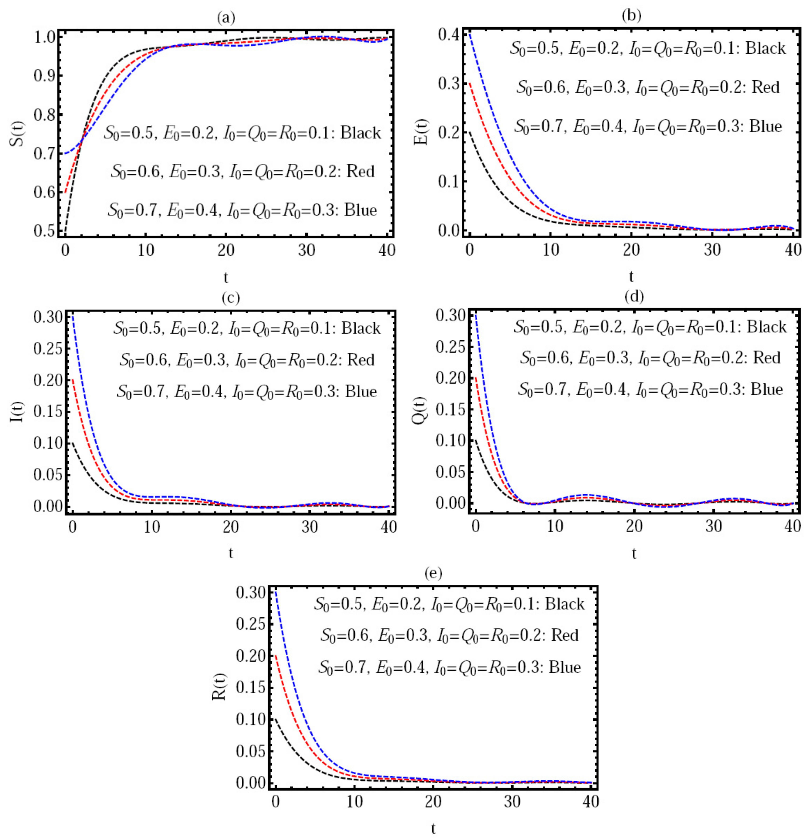
• Figure 4 shows the behavior of the approximate solution with different initial conditions with $m=6,\alpha =0.95$ in the range ($0,40$) and the parameters $ϵ=0.5,{\gamma }_1=1.05,{\gamma }_2=0.005,\varphi =0.5,q_1=0.001,\omega =0.00398,{\rho }_1=0.0047876,{\rho }_2=0.000001231,\alpha =0.085432,\theta =0.09871,\mathrm{\Lambda }=0.1243$; where $S\left(t\right),E\left(t\right),I\left(t\right),Q\left(t\right),R\left(t\right)$ are presented in Figure 4a–e, respectively. In this special case, we take the following different cases:

  i.

  $S_0=0.5,E_0=0.2,I_0=Q_0=R_0=0.1$;

  ii.

  $S_0=0.6,E_0=0.3,I_0=Q_0=R_0=0.2$;

  iii.

  $S_0=0.7,E_0=0.4,I_0=Q_0=R_0=0.3$.

  In all these cases, we note that ${\mathfrak{R}}_0<1$.
• The behavior of the approximate solution via distinct values of $q_1$ with $m=5,\nu =0.98,S_0=0.5,E_0=0.2,I_0=Q_0=R_0=0.1$ in the interval ($0,40$) is presented in Figure 5, and in this case, we take the following cases:

  (1)

  $q_1=0.1,{\mathfrak{R}}_0=0.11143;$

  (2)

  $q_1=0.5,{\mathfrak{R}}_0=0.070515;$

  (3)

  $q_1=0.9,{\mathfrak{R}}_0=0.051577.$

• Furthermore, Figure 6 introduces the residual error function (REF) with $m=7$, $\nu =0.96$, and the same conditions and parameters as Figure 2.
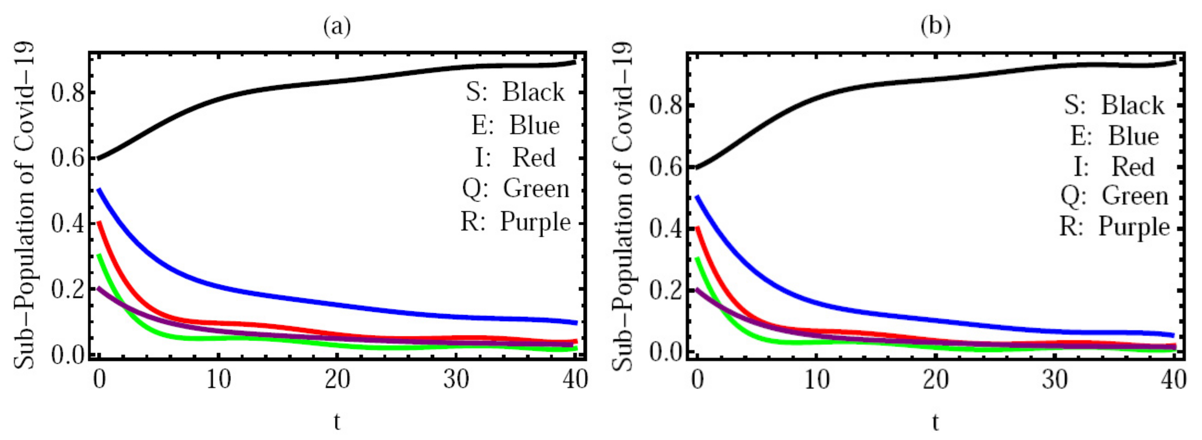
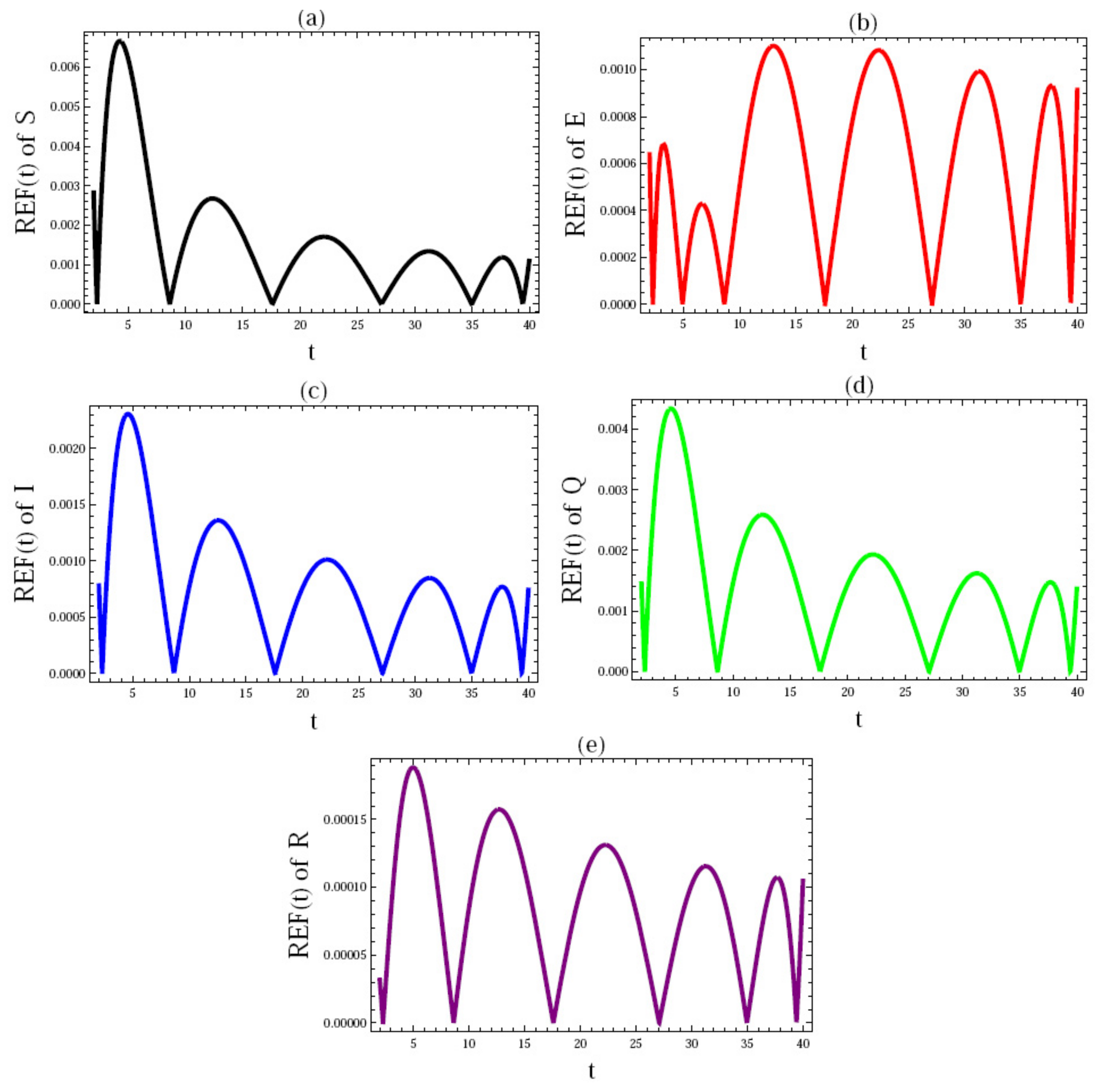
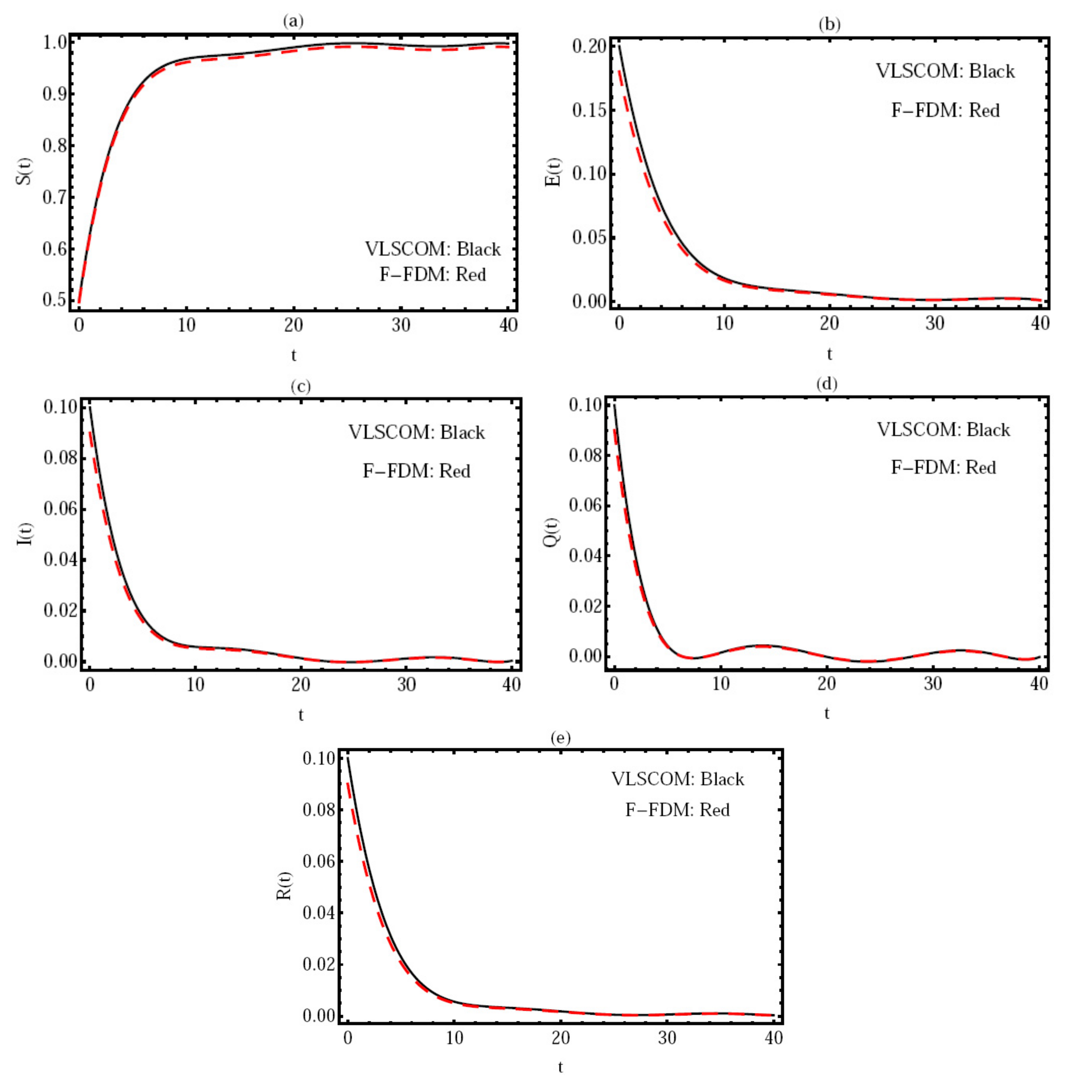
• Finally, for $\nu =0.95$ and $h=0.05$, we showed a comparison between the numerical solution generated by the VLSCOM and the fractional FDM in Figure 7. With the same parameters as in Figure 4, and the same initial conditions as in Figure 4, $S_0=0.5,E_0=0.2,I_0=Q_0=R_0=0.1.$ We can see from this diagram that the theoretical results on stability acquired in the preceding section are correct.
  The behavior of the numerical solution is dependent on the values of $\nu$, m, the initial conditions, and the included parameters $ϵ,{\gamma }_1,{\gamma }_2,\varphi ,q_1,\omega ,{\rho }_1,$${\rho }_2,\alpha ,\theta ,\mathrm{\Lambda }$ as shown in Figure 2, Figure 3, Figure 4, Figure 5 and Figure 6 and this demonstrates that the proposed method is well-implemented for tackling the proposed fractional derivatives problem.

Based on the results, we can see that people’s susceptibility will decrease at constant rates as they come in contact with exposed or infected individuals, leading to a greater number of exposed individuals. As individuals exposed to COVID-19 become infected, decreases and increases. Likewise, as a percentage of recovered individuals die due to natural causes, the number of exposed, infected, and quarantined individuals declines. Furthermore, the number of individuals quarantined in relation to the total number of individuals exposed increases and decreases.

6. Conclusions

The properties of the SVLPs were applied with the SCM to reduce the studied model for the fractional COVID-19 to the solution for a nonlinear system of algebraic equations. The unknown coefficients can be obtained by constructing and solving the resulting system as a restricted optimization problem. The analysis of the convergence of the approximation solution, and the upper bound of the error are stated. The investigated problem’s answers show that the offered technique is quite suitable for studying this topic efficiently. We can also confirm that adding extra terms from the approximate solution’s series reduces the mistakes. Finally, numerical solutions with various values of the included parameters and variables, as well as the REF, are computed to ensure that the suggested technique is valid for such models. Mathematica was used to obtain all numerical results.

We can deduce the following from the numerical simulation presented:

• The proposed method is more reliable and efficient.
• The capacity to obtain accurate results by applying a minimal number of series solution terms.
• This method has various advantages for dealing with problems like this, where the coefficients may be discovered using the Penalty Leap Frog method, and then the approximate solution can be obtained.

Furthermore, we can suggest that by raising public knowledge and encouraging people to follow the government’s instructions, the number of people who are vulnerable to infection is reduced and the number of people who are infected is increased, which helps to lower the severity of infection. Finally, because most numerical methods have restrictions, the fractional FDM has some shortcomings because we can’t assess the solution at any place but the nodes of the provided domain, and it isn’t unconditionally stable. We intend to complete certain future projects, such as:

• Using several techniques to solve the same model;
• Optimal control of the solutions that result;
• Theoretical research to describe the COVID-19 model in depth;
• Change the fractional derivative’s sense to variable-order, for example.

References

- Ahmed, I.; Modu, G.U.; Yusuf, A.; Kumam, P.; Yusuf, I. A mathematical model of Coronavirus Disease (COVID-19) containing asymptomatic and symptomatic classes. Results Phys. 2021, 21, 1–14. [Google Scholar] [CrossRef] [PubMed]
- World Health Organization. Report of the Who-China Joint Mission on Coronavirus Disease; World Health Organization: Geneva, Switzerland, 2020. [Google Scholar]
- Agarwal, P.; Agarwal, R.P.; Ruzhansky, M. Special Functions and Analysis of Differential Equations; Chapman and Hall/CRC: Boca Raton, FL, USA, 2020. [Google Scholar]
- Agarwal, P.; Dragomir, S.S.; Jleli, M.; Samet, B. Advances in Mathematical Inequalities and Applications; Springer Nature: Basel, Germany, 2018. [Google Scholar]
- Ruzhansky, M.; Cho, Y.J.; Agarwal, P.; Area, I. Advances in Real and Complex Analysis with Applications; Trends in Mathematics; Birkhuser: Basel, Switzerland, 2017. [Google Scholar]
- Anderson, R.M.; May, R.M. Helminth infections of humans: Mathematical models, population dynamics, and control. Adv. Parasitol. 1985, 24, 1–101. [Google Scholar] [PubMed]
- Meng, X.; Zhao, S.; Feng, T.; Zhang, T. Dynamics of a novel nonlinear stochastic SIS epidemic model with double epidemic hypothesis. J. Math. Anal. Appl. 2016, 433, 227–242. [Google Scholar] [CrossRef]
- Kabir, K.A.; Kuga, K.; Tanimoto, J. Analysis of SIR epidemic model with information spreading of awareness. Chaos Solitons Fract. 2019, 119, 118–125. [Google Scholar] [CrossRef]
- Khoojine, A.S.; Mahsuli, M.; Shadabfar, M.; Hosseini, V.R.; Kordestani, H. A proposed fractional dynamic system and Monte Carlo-based back analysis for simulating the spreading profile of Covid. Eur. Phys. J. Spec. Top. 2022, 19, 1–11. [Google Scholar]
- Khoojine, A.S.; Mahsuli, M.; Hosseini, V.R.; Kordestani, H. Network autoregressive model for the prediction of COVID-19 considering the disease interaction in neighboring countries. Entropy 2021, 23, 1267. [Google Scholar] [CrossRef]
- Koo, J.R.; Cook, A.R.; Park, M.; Sun, Y.; Sun, H.; Lim, J.T.; Tam, C.; Dickens, B.L. Interventions to mitigate early spread of sars-cov-2 in singapore: A modelling study. Lancet Infect Dis. 2020, 20, 678–688. [Google Scholar] [CrossRef] [Green Version]
- Agarwal, P.; Nieto, J.J.; Ruzhansky, M.; Torres, D.F.M. Analysis of Infectious Disease Problems (COVID-19) and Their Global Impact; Springer: Singapore, 2021. [Google Scholar]
- Rajchakit, G.; Agarwal, P.; Ramalingam, S. Stability Analysis of Neural Networks; Springer: Singapore, 2021. [Google Scholar]
- Rehman, A.U.; Singh, R.; Agarwal, P. Modeling, analysis and prediction of new variants of COVID-19 and dengue co-infection on complex network. Chaos Solitons Fractals 2021, 150, 111008. [Google Scholar] [CrossRef]
- Shadabfar, M.; Mahsuli, M.; Khoojine, A.S.; Hosseini, V.R. Time-variant reliability-based prediction of COVID-19 spread using extended SEIVR model and Monte Carlo sampling. Results Phys. 2021, 26, 1–10. [Google Scholar] [CrossRef]
- Wilder-Smith, A.; Freedman, D.O. Isolation, quarantine, social distancing and community containment: Pivotal role for old-style public health measures in the novel coronavirus (2019-ncov) outbreak. J. Travel Med. 2020, 27, 1–4. [Google Scholar] [CrossRef]
- Agarwal, P.; Baleanu, D.; Chen, Y.; Momani, S.; Machado, J.A.T. Fractional Calculus: ICFDA, 1st ed; Springer Proceedings in Mathematics Statistics; Springer: Singapore, 2019; Volume 303. [Google Scholar]
- Alderremy, A.A.; Saad, K.M.; Agarwal, P.; Aly, S.; Jain, S. Certain new models of the multi space-fractional Gardner equation. Phys. A Stat. Mech. Its Appl. 2020, 545, 123806. [Google Scholar] [CrossRef]
- Kilbas, S.G.; Kilbas, A.A.; Marichev, O.I. Fractional Integrals and Derivatives: Theory and Applications; Gordon & Breach: Yverdon, Switzerland, 1993. [Google Scholar]
- Podlubny, I. Fractional Differential Equations; Academic Press: New York, NY, USA, 1999. [Google Scholar]
- Adel, M.; Elsaid, M. An Efficient Approach for solving fractional variable order reaction sub-diffusion equation base on Hermite formula. Complex Geom. Patterns Scaling Nat. Soc. 2022, 30, 2240020. [Google Scholar]
- Khader, M.M.; Gomez-Aguilar, J.F.; Adel, M. Numerical study for the fractional RL, RC, and RLC electrical circuits using Legendre pseudo-spectral method. Int. J. Circuit Theory Appl. 2021, 49, 1–20. [Google Scholar] [CrossRef]
- Abdeljawad, T.; Baleanu, D. Integration by parts and its applications of a new nonlocal fractional derivative with Mittag-Leffler nonsingular kernel. Nonlin. Sci. Appl. 2017, 9, 1098–1107. [Google Scholar] [CrossRef] [Green Version]
- Diethelm, K.; Ford, N.J.; Freed, A.D. A predictor-corrector approach for the numerical solution of fractional differential equations. Nonlinear Dyn. 2002, 29, 3–22. [Google Scholar] [CrossRef]
- Khader, M.M.; Adel, M. Numerical and theoretical treatment based on the compact finite difference and spectral collocation algorithms of the space fractional-order Fisher’s equation. Int. J. Mod. Phys. C 2020, 31, 1–13. [Google Scholar] [CrossRef]
- Agarwal, P.; El-Sayed, A.A. Vieta-Lucas polynomials for solving a fractional-order mathematical physics model. Adv. Differ. Equ. 2020, 2020, 1–18. [Google Scholar] [CrossRef]
- Jafari, H.; Khalique, C.M.; Nazari, M. An algorithm for the numerical solution of nonlinear fractional-order Van der Pol oscillator equation. Math. Comput. Model. 2012, 55, 1782–1786. [Google Scholar] [CrossRef]
- Sultana, F.; Singh, D.; Pandey, R.K.; Zeidan, D. Numerical schemes for a class of tempered fractional integro-differential equations. Appl. Numer. Math. 2020, 157, 110–134. [Google Scholar] [CrossRef]
- Khader, M.M.; Adel, M. Chebyshev wavelet procedure for solving FLDEs. Acta Appl. Math. 2018, 158, 1–10. [Google Scholar] [CrossRef]
- Khader, M.M.; Adel, M. Numerical approach for solving the Riccati and Logistic equations via QLM-rational Legendre collocation method. Comput. Appl. Math. 2020, 39, 1–9. [Google Scholar] [CrossRef]
- Horadam, A.F. Vieta Polynomials; The University of New England: Armidaie, Australia, 2000; p. 2351. [Google Scholar]
- Kostrzewski, M. Sensitivity analysis of selected parameters in the order picking process simulation model, with randomly generated orders. Entropy 2020, 22, 423. [Google Scholar] [CrossRef] [Green Version]
- Nieto, J.J. Solution of a fractional logistic ordinary differential equation. Appl. Math. Lett. 2022, 123, 107568. [Google Scholar] [CrossRef]
- Rafiq, M.; Macias-Diaz, J.E.; Raza, A.; Ahmed, N. Design of a nonlinear model for the propagation of COVID-19 and its efficient nonstandard computational implementation. Appl. Math. Model. 2021, 89, 1835–1846. [Google Scholar] [CrossRef]
- Diekmann, O.; Heesterbeek, J.A.P.; Metz, J.A. On the definition and the computation of the basic reproduction ratio R0 in models for infectious diseases in heterogeneous populations. J. Math. Biol. 1990, 14, 365–382. [Google Scholar]
- Odibat, Z.M.; Shawagfeh, N.T. Generalized Taylor’s formula. Appl. Math. Comput. 2007, 186, 286–293. [Google Scholar] [CrossRef]
- Reyna, J.A. A generalized mean-value theorem. Monatshefte Math. 1988, 106, 95–97. [Google Scholar] [CrossRef]
- Lin, W. Global existence theory and chaos control of fractional differential equations. J. Math. Anal. Appl. 2007, 332, 709–726. [Google Scholar] [CrossRef] [Green Version]
- Kumar, R.; Kumar, S. A new fractional modelling on Susceptible-Infected-Recovered equations with constant vaccination rate. Nonlinear Eng. 2014, 3, 11–16. [Google Scholar] [CrossRef]
- Matignon, D. Stability results for fractional differential equations with applications to control processing. Comput. Eng. Syst. Appl. 1996, 2, 963–968. [Google Scholar]
- Khan, M.A.; Atangana, A. Modeling the dynamics of novel Coronavirus (2019-nCoV) with fractional derivative. Alex. Eng. J. 2020, 59, 2379–2389. [Google Scholar] [CrossRef]
- El-Hawary, H.M.; Salim, M.S.; Hussien, H.S. Ultraspherical integral method for optimal control problems governed by ordinary differential equations. J. Glob. Optim. 2003, 25, 283–303. [Google Scholar] [CrossRef]
Publisher’s Note: MDPI stays neutral with regard to jurisdictional claims in published maps and institutional affiliations. |
© 2022 by the authors. Licensee MDPI, Basel, Switzerland. This article is an open access article distributed under the terms and conditions of the Creative Commons Attribution (CC BY) license (https://creativecommons.org/licenses/by/4.0/).
Share and Cite
Khader, M.M.; Adel, M. Modeling and Numerical Simulation for Covering the Fractional COVID-19 Model Using Spectral Collocation-Optimization Algorithm. Fractal Fract. 2022, 6, 363. https://0-doi-org.brum.beds.ac.uk/10.3390/fractalfract6070363
Khader MM, Adel M. Modeling and Numerical Simulation for Covering the Fractional COVID-19 Model Using Spectral Collocation-Optimization Algorithm. Fractal and Fractional. 2022; 6(7):363. https://0-doi-org.brum.beds.ac.uk/10.3390/fractalfract6070363
Chicago/Turabian StyleKhader, Mohamed M., and Mohamed Adel. 2022. "Modeling and Numerical Simulation for Covering the Fractional COVID-19 Model Using Spectral Collocation-Optimization Algorithm" Fractal and Fractional 6, no. 7: 363. https://0-doi-org.brum.beds.ac.uk/10.3390/fractalfract6070363