Low-Cost Multispectral Sensor Array for Determining Leaf Nitrogen Status

 ,
,  ,
,  and
and
Abstract
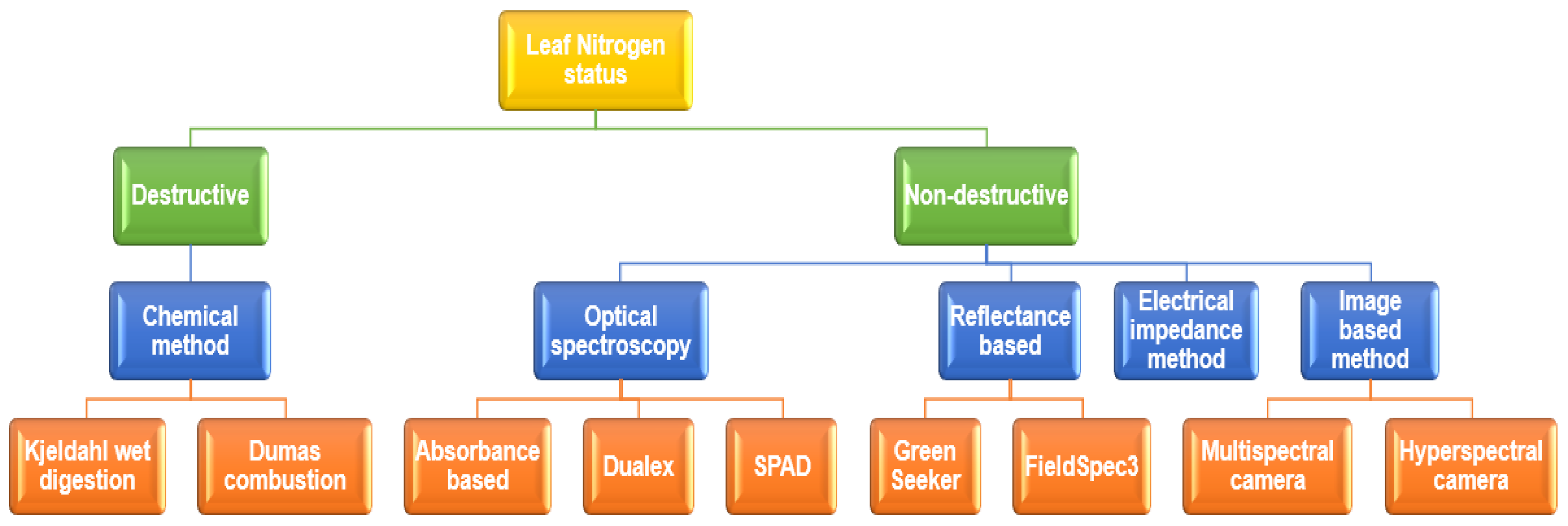
:1. Introduction
2. Materials and Methods
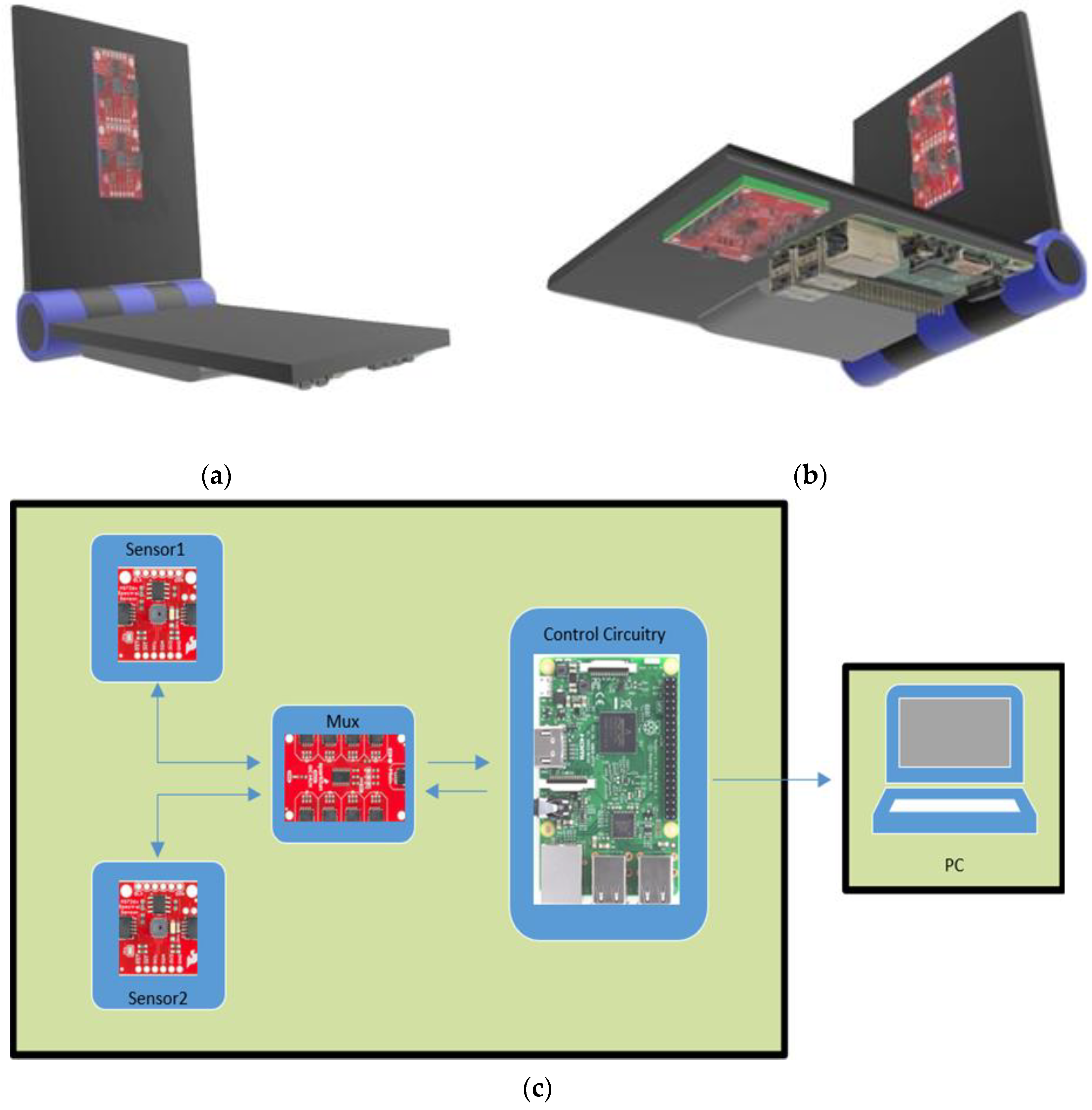
2.1. Designed Hardware for N Sensing System
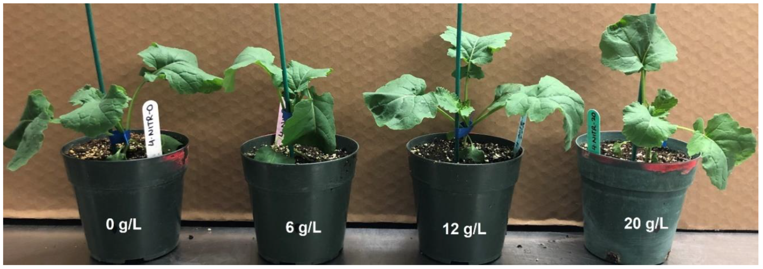
2.2. Greenhouse Experimental Setup
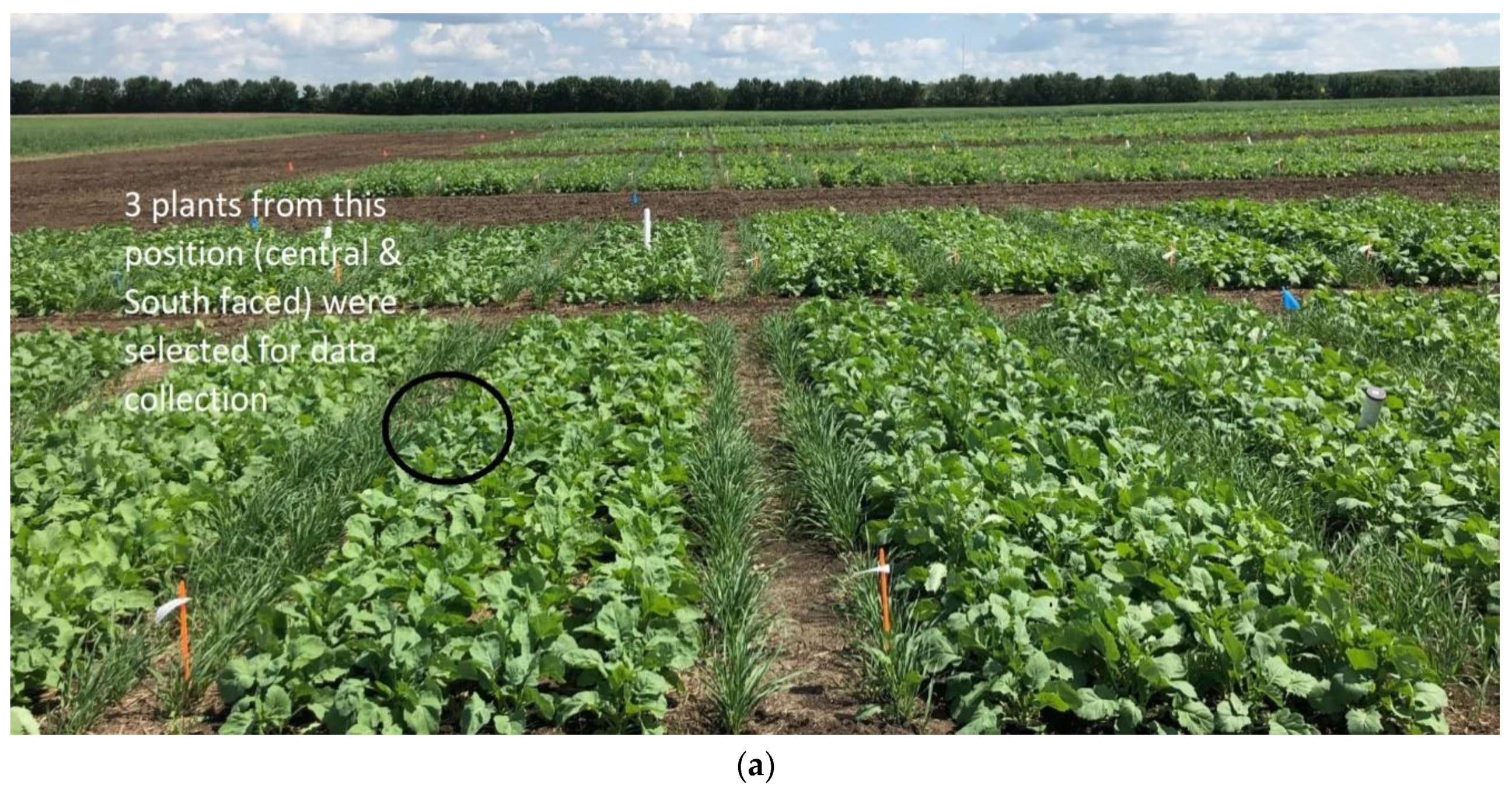
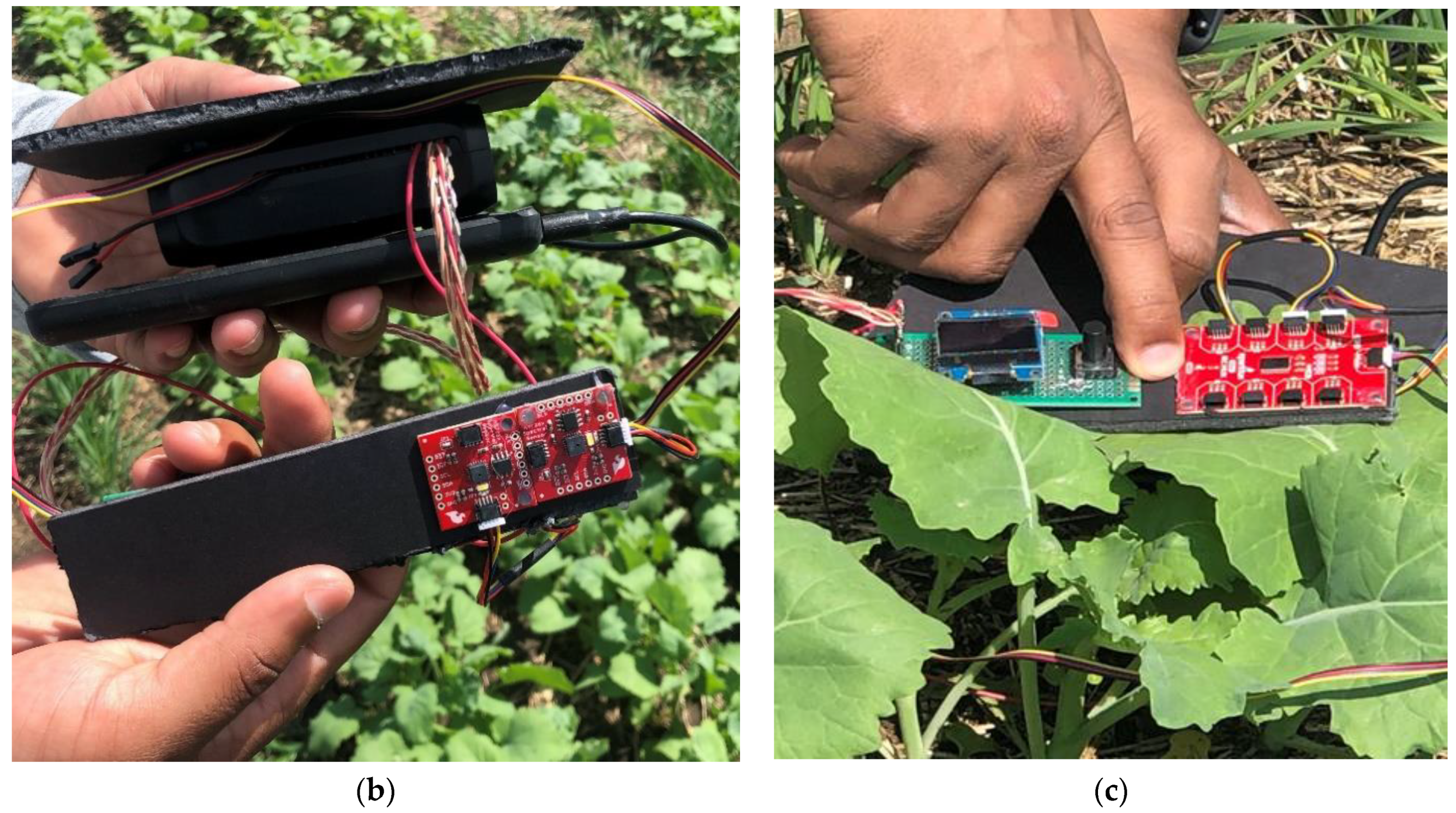
2.3. Field Experiment Setup
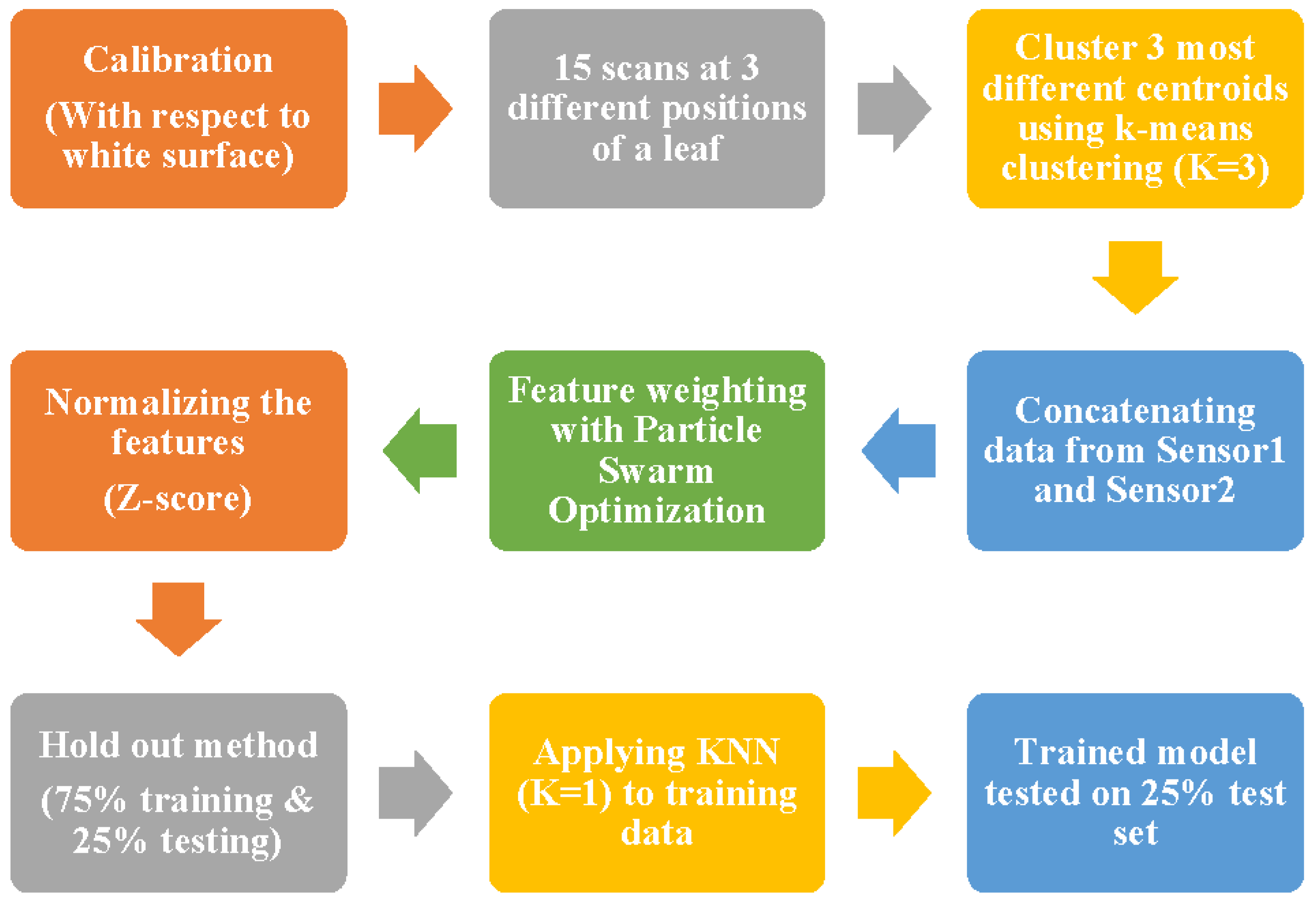
2.4. Data Collection and Modeling
2.5. Evaluation Metrics
3. Result and Discussion
4. Conclusions
Supplementary Materials
Author Contributions
Funding
Acknowledgments
Conflicts of Interest
References
- Wang, L.; Macko, S.A. Constrained preferences in nitrogen uptake across plant species and environments. Plant. Cell Environ. 2011, 34, 525–534. [Google Scholar] [CrossRef] [PubMed]
- Sinfield, J.V.; Fagerman, D.; Colic, O. Evaluation of sensing technologies for on-the-go detection of macro-nutrients in cultivated soils. Comput. Electron. Agric. 2010, 70, 1–18. [Google Scholar] [CrossRef]
- Vigneau, N.; Ecarnot, M.; Rabatel, G.; Roumet, P. Potential of field hyperspectral imaging as a non destructive method to assess leaf nitrogen content in wheat. Field Crop. Res. 2011, 122, 25–31. [Google Scholar] [CrossRef] [Green Version]
- Padilla, F.M.; Gallardo, M.; Peña-Fleitas, M.T.; de Souza, R.; Thompson, R.B. Proximal optical sensors for nitrogen management of vegetable crops: A review. Sensors 2018, 18, 2083. [Google Scholar] [CrossRef] [PubMed] [Green Version]
- Xiong, D.; Chen, J.; Yu, T.; Gao, W.; Ling, X.; Li, Y.; Peng, S.; Huang, J. SPAD-based leaf nitrogen estimation is impacted by environmental factors and crop leaf characteristics. Sci. Rep. 2015, 5, 1–12. [Google Scholar] [CrossRef] [Green Version]
- Berger, K.; Verrelst, J.; Féret, J.-B.; Wang, Z.; Wocher, M.; Strathmann, M.; Danner, M.; Mauser, W.; Hank, T. Crop nitrogen monitoring: Recent progress and principal developments in the context of imaging spectroscopy missions. Remote Sens. Environ. 2020, 242, 111758. [Google Scholar] [CrossRef]
- Osborne, S.L.; Schepers, J.S.; Francis, D.D.; Schlemmer, M.R. Detection of phosphorus and nitrogen deficiencies in corn using spectral radiance measurements. Agron. J. 2002, 94, 1215. [Google Scholar] [CrossRef] [Green Version]
- Wang, J.; Shen, C.; Liu, N.; Jin, X.; Fan, X.; Dong, C.; Xu, Y. Non-destructive evaluation of the leaf nitrogen concentration by in-field visible/near-infrared spectroscopy in Pear Orchards. Sensors 2017, 17, 538. [Google Scholar] [CrossRef] [Green Version]
- Barbedo, J.G.A. Detection of nutrition deficiencies in plants using proximal images and machine learning: A review. Comput. Electron. Agric. 2019, 162, 482–492. [Google Scholar] [CrossRef]
- Muñoz-Huerta, R.F.; Guevara-Gonzalez, R.G.; Contreras-Medina, L.M.; Torres-Pacheco, I.; Prado-Olivarez, J.; Ocampo-Velazquez, R.V. A review of methods for sensing the nitrogen status in plants: Advantages, disadvantages and recent advances. Sensors 2013, 13, 10823–10843. [Google Scholar] [CrossRef]
- Mercado-Luna, A.; Rico-García, E.; Lara-Herrera, A.; Soto-Zarazúa, G.; Ocampo-Velázquez, R.; Guevara-González, R.; Herrera-Ruiz, G.; Torres-Pacheco, I. Nitrogen determination on tomato (Lycopersicon esculentum Mill.) seedlings by color image analysis (RGB). Afr. J. Biotechnol. 2010, 9, 5326–5332. [Google Scholar]
- Yu, K.Q.; Zhao, Y.R.; Li, X.L.; Shao, Y.N.; Liu, F.; He, Y. Hyperspectral imaging for mapping of total nitrogen spatial distribution in pepper plant. PLoS ONE 2014, 9, e116205. [Google Scholar] [CrossRef] [PubMed]
- Krutz, D.; Müller, R.; Knodt, U.; Günther, B.; Walter, I.; Sebastian, I.; Säuberlich, T.; Reulke, R.; Carmona, E.; Eckardt, A.; et al. The Instrument Design of the DLR Earth Sensing Imaging Spectrometer (DESIS). Sensors 2019, 19, 1622. [Google Scholar] [CrossRef] [PubMed] [Green Version]
- Guanter, L.; Kaufmann, H.; Segl, K.; Foerster, S.; Rogass, C.; Chabrillat, S.; Kuester, T.; Hollstein, A.; Rossner, G.; Chlebek, C.; et al. The EnMAP spaceborne imaging spectroscopy mission for earth observation. Remote Sens. 2015, 7, 8830–8857. [Google Scholar] [CrossRef] [Green Version]
- Staenz, K.; Mueller, A.; Heiden, U. Overview of terrestrial imaging spectroscopy missions. In Proceedings of the 2013 IEEE International Geoscience and Remote Sensing Symposium-IGARSS, Melbourne, VIC, Australia, 21–26 July 2013; pp. 3502–3505. [Google Scholar]
- Tomkiewicz, D.; Piskier, T. A plant based sensing method for nutrition stress monitoring. Precis. Agric. 2012, 13, 370–383. [Google Scholar] [CrossRef]
- Blackmer, T.; Schepers, J.S. Techniques for monitoring crop nitrogen status in corn. Commun. Soil Sci. Plant Anal. 1994, 25, 1791–1800. [Google Scholar] [CrossRef]
- Wang, L.; Okin, G.S.; Wang, J.; Epstein, H.; Macko, S.A. Predicting leaf and canopy 15N compositions from reflectance spectra. Geophys. Res. Lett. 2007, 34, L02401. [Google Scholar]
- Stone, M.L.; Solie, J.B.; Raun, W.R.; Whitney, R.W.; Taylor, S.L.; Ringer, J.D. Use of spectral radiance for correcting in-season fertilizer nitrogen deficiencies in winter wheat. Trans. Am. Soc. Agric. Eng. 1996, 39, 1623–1631. [Google Scholar] [CrossRef]
- Zhang, X.; Liu, F.; He, Y.; Gong, X. Detecting macronutrients content and distribution in oilseed rape leaves based on hyperspectral imaging. Biosyst. Eng. 2013, 115, 56–65. [Google Scholar] [CrossRef]
- Lawes, R.A.; Oliver, Y.M.; Huth, N.I. Optimal nitrogen rate can be predicted using average yield and estimates of soil water and leaf nitrogen with infield experimentation. Agron. J. 2019, 111, 1155–1164. [Google Scholar] [CrossRef]
- Chlingaryan, A.; Sukkarieh, S.; Whelan, B. Machine learning approaches for crop yield prediction and nitrogen status estimation in precision agriculture: A review. Comput. Electron. Agric. 2018, 151, 61–69. [Google Scholar] [CrossRef]
- Sun, J.; Yang, J.; Shi, S.; Chen, B.; Du, L.; Gong, W.; Song, S. Estimating Rice Leaf Nitrogen Concentration: Influence of Regression Algorithms Based on Passive and Active Leaf Reflectance. Remote Sens. 2017, 9, 951. [Google Scholar] [CrossRef] [Green Version]
- Pattern Recognition and Machine Learning. J. Electron. Imaging 2007, 16, 049901. [CrossRef] [Green Version]
- Griffiths, T.L.; Ghahramani, Z. The Indian buffet process: An introduction and review. J. Mach. Learn. Res. 2011, 12, 1185–1224. [Google Scholar]
- Mulla, D.J. Twenty five years of remote sensing in precision agriculture: Key advances and remaining knowledge gaps. Biosyst. Eng. 2013, 114, 358–371. [Google Scholar] [CrossRef]
- SparkFun Spectral Sensor Breakout AS7262 Visible (Qwiic)-SEN-14347-SparkFun Electronics. Available online: https://www.sparkfun.com/products/14347 (accessed on 25 February 2020).
- Single-Chip Spectrometers | DigiKey. Available online: https://www.digikey.be/en/articles/techzone/2017/jun/optical-sensor-on-chip-ics-simplify-handheld-spectrometer-design (accessed on 27 August 2019).
- AS7263 6-Channel Spectrometer-Ams | Mouser Canada. Available online: https://www.mouser.ca/new/ams/ams-as7263-spectral-id-device/ (accessed on 27 August 2019).
- Amazon.com. Raspberry Pi 3 Model B Board: Computers & Accessories. Available online: https://www.amazon.com/Raspberry-Pi-MS-004-00000024-Model-Board/dp/B01LPLPBS8 (accessed on 25 January 2020).
- Senthilkumar, G.; Gopalakrishnan, K.; Satish, K. Embedded image capturing system using raspberry pi system. Int. J. Emerg. Trends Technol. Comput. Sci. 2014, 3, 213–215. [Google Scholar]
- Imteaj, A.; Rahman, T.; Hossain, M.K.; Alam, M.S.; Rahat, S.A. An IoT based fire alarming and authentication system for workhouse using Raspberry Pi 3. In Proceedings of the 2017 International Conference on Electrical, Computer and Communication Engineering (ECCE), Cox’s Bazar, Bangladesh, 16–18 February 2017; pp. 899–904. [Google Scholar]
- Agrawal, N.; Singhal, S. Smart drip irrigation system using raspberry pi and arduino. Int. Conf. Comput. Commun. Autom. 2015, 928–932. [Google Scholar]
- Paper Mirror. Available online: https://www.amazon.ca/Cloakroom-Decorative-Background-Removable-Self-Adhesive/dp/B07W312F98/ref=asc_df_B07W312F98/?tag=googleshopc0c-20&linkCode=df0&hvadid=335179893508&hvpos=1o2&hvnetw=g&hvrand=6497894200531816537&hvpone=&hvptwo=&hvqmt=&hvdev=c&hvdvcmdl= (accessed on 4 February 2020).
- Jain, A.K. Data clustering: 50 years beyond K-means. Pattern Recognit. Lett. 2010, 31, 651–666. [Google Scholar] [CrossRef]
- Rodriguez-Galiano, V.F.; Luque-Espinar, J.A.; Chica-Olmo, M.; Mendes, M.P. Feature selection approaches for predictive modelling of groundwater nitrate pollution: An evaluation of filters, embedded and wrapper methods. Sci. Total Environ. 2018, 624, 661–672. [Google Scholar] [CrossRef]
- Pourmohammadali, B.; Salehi, M.H.; Hosseinifard, S.J.; Esfandiarpour Boroujeni, I.; Shirani, H. Studying the relationships between nutrients in pistachio leaves and its yield using hybrid GA-ANN model-based feature selection. Comput. Electron. Agric. 2020, 172, 105352. [Google Scholar] [CrossRef]
- Habibullah, M.; Mohebian, M.R.; Soolanayakanahally, R.; Wahid, K.A.; Dinh, A. A cost-effective and portable optical sensor system to estimate leaf nitrogen and water contents in crops. Sensors 2020, 20, 1449. [Google Scholar] [CrossRef] [PubMed] [Green Version]
- Borda, R.P.; Frost, J.D. Error reduction in small sample averaging through the use of the median rather than the mean. Electroencephalogr. Clin. Neurophysiol. 1968, 25, 391–392. [Google Scholar] [CrossRef]
- Kumar, R.R.; Viswanath, P.; Bindu, C.S. Nearest neighbor classifiers: Reducing the computational demands. In Proceedings of the 2016 IEEE 6th International Conference on Advanced Computing (IACC), Bhimavaram, India, 27–28 February 2016; pp. 45–50. [Google Scholar]
- Mallah, C.; Cope, J.; Orwell, J. Plant leaf classification using probabilistic integration of shape, texture and margin features. In Proceedings of the IASTED International Conference on Signal Processing, Pattern Recognition and Applications, Innsbruck, Austria, 12–14 February 2013. [Google Scholar]
- Parry, R.M.; Jones, W.; Stokes, T.H.; Phan, J.H.; Moffitt, R.A.; Fang, H.; Shi, L.; Oberthuer, A.; Fischer, M.; Tong, W.; et al. K-Nearest neighbor models for microarray gene expression analysis and clinical outcome prediction. Pharm. J. 2010, 10, 292–309. [Google Scholar] [CrossRef] [Green Version]
- Wu, K.-P.; Wang, S.-D. Choosing the kernel parameters for support vector machines by the inter-cluster distance in the feature space. Pattern Recognit. 2009, 42, 710–717. [Google Scholar] [CrossRef]
- Rumpf, T.; Mahlein, A.-K.; Steiner, U.; Oerke, E.C.; Dehne, H.W.; Plümer, L. Early detection and classification of plant diseases with Support Vector Machines based on hyperspectral reflectance. Comput. Electron. Agric. 2010, 74, 91–99. [Google Scholar] [CrossRef]
- Verrelst, J.; Camps-Valls, G.; Muñoz-Marí, J.; Rivera, J.P.; Veroustraete, F.; Clevers, J.G.P.W.; Moreno, J. Optical remote sensing and the retrieval of terrestrial vegetation bio-geophysical properties–A review. ISPRS J. Photogramm. Remote Sens. 2015, 108, 273–290. [Google Scholar] [CrossRef]
- Salzberg, S.L. C4.5: Programs for Machine Learning by J. Ross Quinlan; Morgan Kaufmann Publishers: Burlington, MA, USA, 1994; Volume 16, pp. 235–240. [Google Scholar]
- Banfield, R.E.; Hall, L.O.; Bowyer, K.W.; Kegelmeyer, W.P. A comparison of decision tree ensemble creation techniques. IEEE Trans. Pattern Anal. Mach. Intell. 2007, 29, 173–180. [Google Scholar] [CrossRef]
- Sokolova, M.; Lapalme, G. A systematic analysis of performance measures for classification tasks. Inf. Process. Manag. 2009, 45, 427–437. [Google Scholar] [CrossRef]
- Palaniappan, R.; Sundaraj, K.; Sundaraj, S. A comparative study of the svm and k-nn machine learning algorithms for the diagnosis of respiratory pathologies using pulmonary acoustic signals. BMC Bioinform. 2014, 15, 223. [Google Scholar] [CrossRef] [Green Version]
- Wang, F.; Zhen, Z.; Wang, B.; Mi, Z. Comparative study on KNN and SVM based weather classification models for day ahead short term solar PV power forecasting. Appl. Sci. 2017, 8, 28. [Google Scholar] [CrossRef] [Green Version]
- McInerney, D.O.; Nieuwenhuis, M. A comparative analysis of k NN and decision tree methods for the Irish National Forest Inventory. Int. J. Remote Sens. 2009, 30, 4937–4955. [Google Scholar] [CrossRef]
- Homolová, L.; Malenovský, Z.; Clevers, J.G.P.W.; García-Santos, G.; Schaepman, M.E. Review of optical-based remote sensing for plant trait mapping. Ecol. Complex. 2013, 15, 1–16. [Google Scholar] [CrossRef] [Green Version]
- Herrmann, I.; Karnieli, A.; Bonfil, D.J.; Cohen, Y.; Alchanatis, V. SWIR-based spectral indices for assessing nitrogen content in potato fields. Int. J. Remote Sens. 2010, 31, 5127–5143. [Google Scholar] [CrossRef]
- Curran, P.J. Remote sensing of foliar chemistry. Remote Sens. Environ. 1989, 3, 271–278. [Google Scholar] [CrossRef]
- Kumar, L.; Schmidt, K.; Dury, S.; Skidmore, A. Imaging Spectrometry and Vegetation Science. In Imaging Spectrometry; Van Der Meer, F.D., De Jong, S.M., Eds.; Kluwer Academic, Springer: Dordrecht, Germany, 2006; pp. 111–155. [Google Scholar]
- Fourty, T.; Baret, F.; Jacquemoud, S.; Schmuck, G.; Verdebout, J. Leaf optical properties with explicit description of its biochemical composition: Direct and inverse problems. Remote Sens. Environ. 1996, 56, 104–117. [Google Scholar] [CrossRef]


| Hardware Components | Summary of the Technical Specifications |
|---|---|
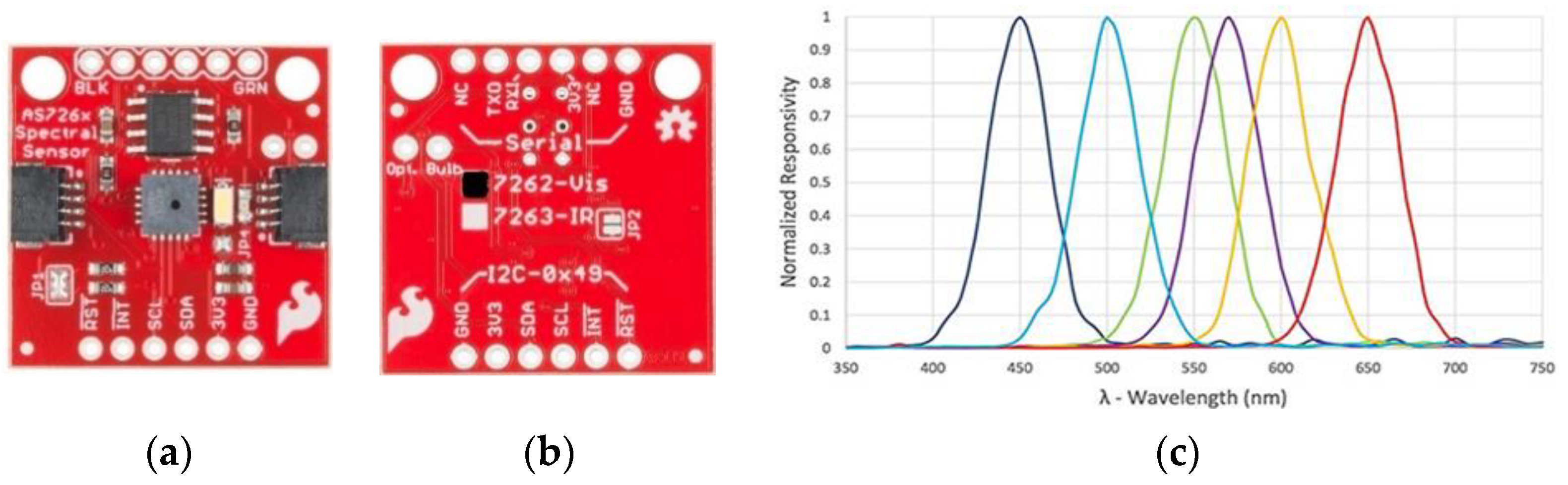
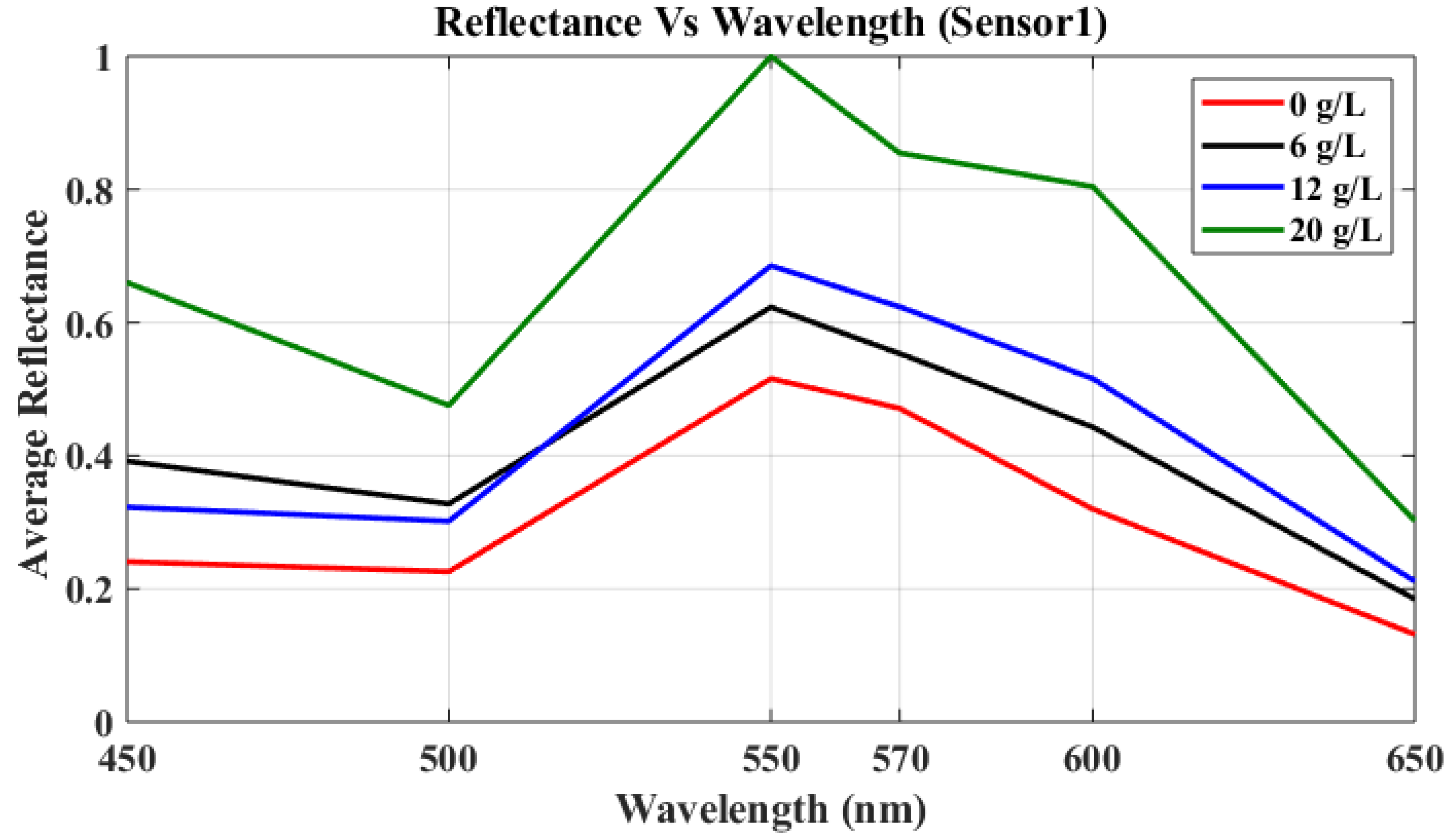
| Sensor1 (SEN-14347) | 6 channel multi-spectral sensor in the visible range (450, 500, 550, 570, 600, 650 nm). The measurement unit of the channel is μW/. Built-in source light (5700 K white LED) |
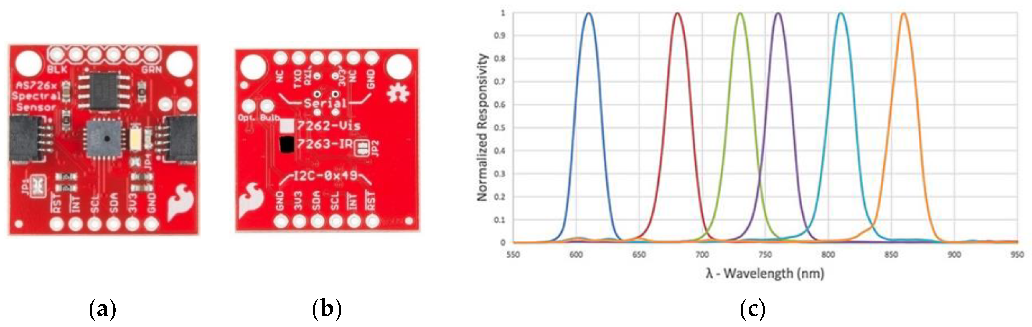
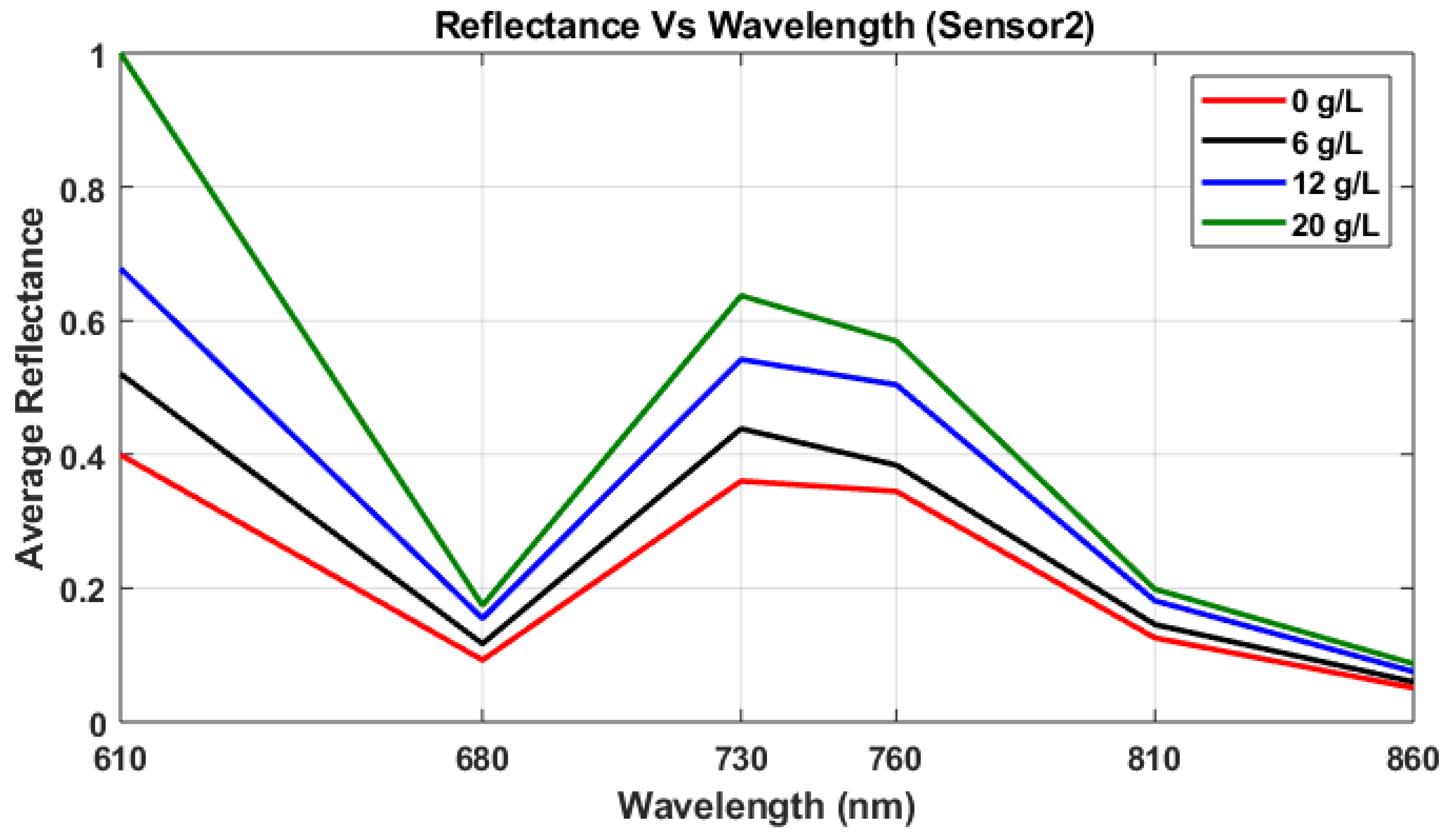
| Sensor2 (SEN-14351) | 6 channel multi-spectral sensor in the NIR range (610, 680, 730, 760, 810, and 860 nm). The measurement unit of the channel is μW/. Onboard source light is a 2700 K warm LED |
| Microprocessor-based control circuitry | Raspberry Pi 3 model B. 1.2 GHz AR processor. 1 GB LPDDR2 main memory |
| Multiplexer | 8 configurable addresses |
| Accuracy (%) | Precision (%) | Recall (%) | Specificity (%) | F1-Score (%) | |
|---|---|---|---|---|---|
| Category1 | 92.8 ± 1.5 | 81.2 ± 2.1 | 92.8 ± 1.2 | 92.1 ± 1.1 | 86.6 ± 2.2 |
| Category2 | 71.4 ± 1.1 | 99.9 ± 0.2 | 71.4 ± 2.0 | 100 ± 0.0 | 83.3 ± 2.5 |
| Category3 | 90.9 ± 3.1 | 99.9 ± 0.1 | 90.9 ± 1.6 | 100 ± 0.0 | 95.2 ± 1.6 |
| Category4 | 99.9 ± 0.1 | 81.2 ± 1.5 | 99.9 ± 0.3 | 92.3 ± 1.3 | 89.6 ± 1.8 |
| Total | 88.4 ± 3.0 | 90.6 ± 2.3 | 88.8 ± 2.9 | 96.1 ± 2.0 | 88.7 ± 2.6 |
| Environment | Accuracy (%) | Precision (%) | Recall (%) | Specificity (%) | F1-Score (%) |
|---|---|---|---|---|---|
| Greenhouse | 94.2 ± 1.8 | 90.9 ± 2.1 | 100.0 ± 0.0 | 90.9 ± 1.9 | 95.2 ± 1.8 |
| Field | 79.2 ± 2.5 | 80.1 ± 2.7 | 79.6 ± 2.1 | 80.2 ± 2.3 | 79.3 ± 2.4 |
| Training Algorithms | Testing Accuracy (%) of the Greenhouse Experiment | Testing Accuracy (%) of Field Experiment |
|---|---|---|
| Decision Tree | 65.1 ± 2.7 | 73.6 ± 2.6 |
| Support Vector Machine (SVM) | 65.0 ± 2.0 | 70.1 ± 2.1 |
| Ensemble Bagged Tree | 73.3 ± 2.2 | 75.0 ± 2.3 |
| K-Nearest Neighbor (KNN) | 88.4 ± 3.0 | 79.2 ± 2.5 |
© 2020 by the authors. Licensee MDPI, Basel, Switzerland. This article is an open access article distributed under the terms and conditions of the Creative Commons Attribution (CC BY) license (http://creativecommons.org/licenses/by/4.0/).
Share and Cite
Habibullah, M.; Mohebian, M.R.; Soolanayakanahally, R.; Bahar, A.N.; Vail, S.; Wahid, K.A.; Dinh, A. Low-Cost Multispectral Sensor Array for Determining Leaf Nitrogen Status. Nitrogen 2020, 1, 67-80. https://0-doi-org.brum.beds.ac.uk/10.3390/nitrogen1010007
Habibullah M, Mohebian MR, Soolanayakanahally R, Bahar AN, Vail S, Wahid KA, Dinh A. Low-Cost Multispectral Sensor Array for Determining Leaf Nitrogen Status. Nitrogen. 2020; 1(1):67-80. https://0-doi-org.brum.beds.ac.uk/10.3390/nitrogen1010007
Chicago/Turabian StyleHabibullah, Mohammad, Mohammad Reza Mohebian, Raju Soolanayakanahally, Ali Newaz Bahar, Sally Vail, Khan A. Wahid, and Anh Dinh. 2020. "Low-Cost Multispectral Sensor Array for Determining Leaf Nitrogen Status" Nitrogen 1, no. 1: 67-80. https://0-doi-org.brum.beds.ac.uk/10.3390/nitrogen1010007