Machining Quality Prediction Using Acoustic Sensors and Machine Learning †

 and
and
Abstract
:1. Introduction
Theoretical Background
2. Materials, Methods and Data Acquisition
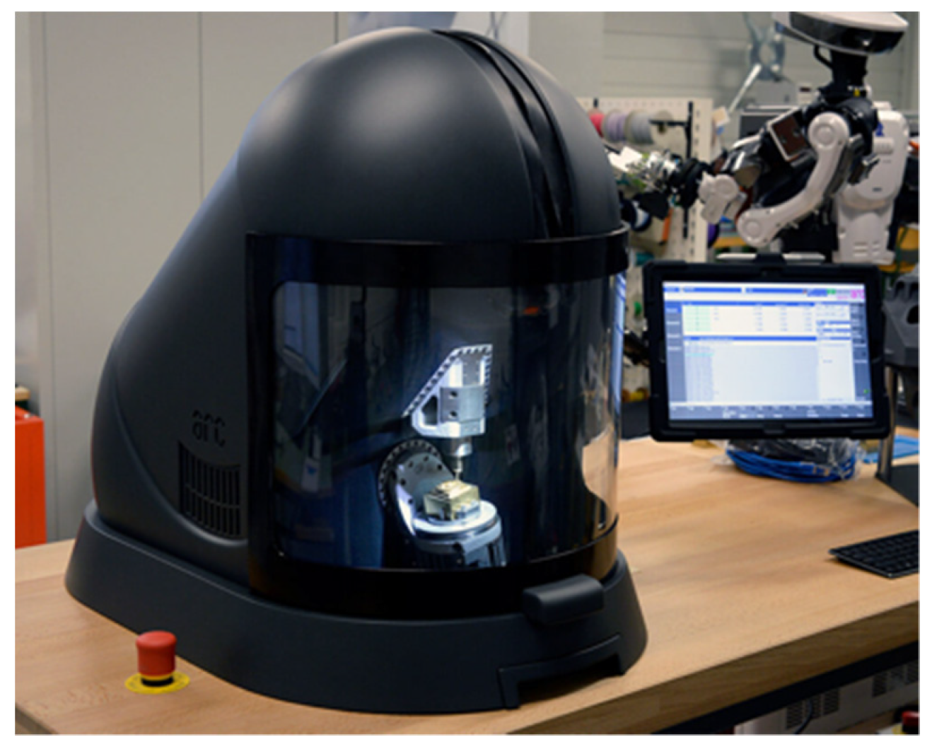
2.1. Materials
2.2. Methodology: Data Acquisition, Labeling and Classification
- label=0.
- the tool breaks;
- lbbel=0.
- the tool is considered ‘too used’ by an expert human;
- lcbel=0.
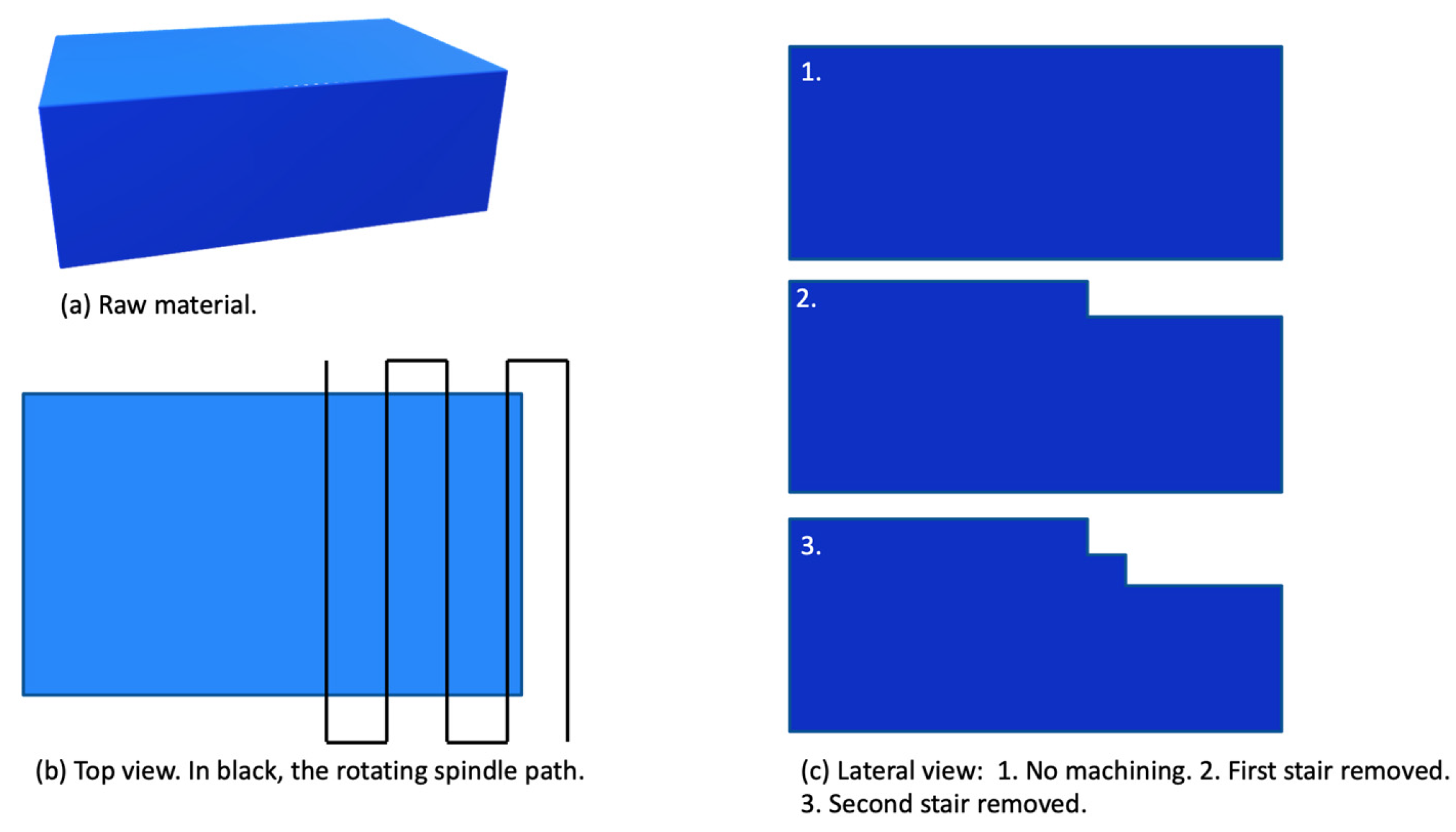
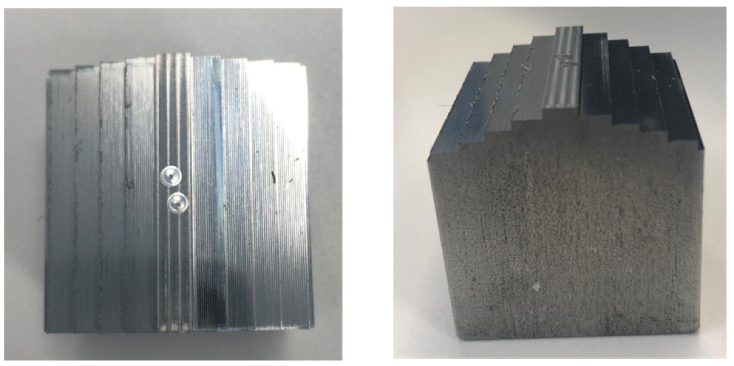
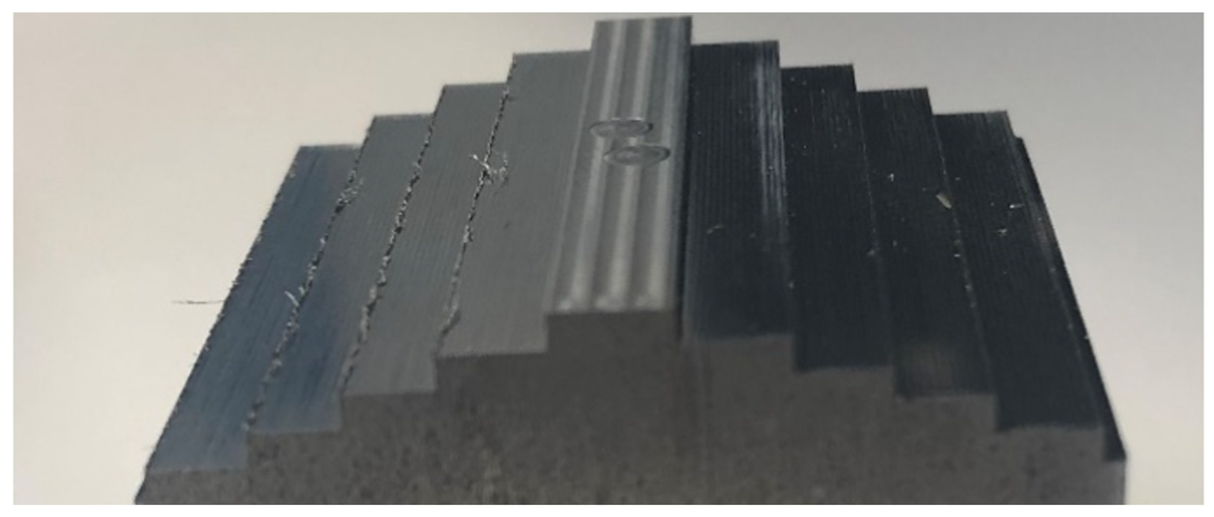
- the workpiece is completely machined (6 stairs).
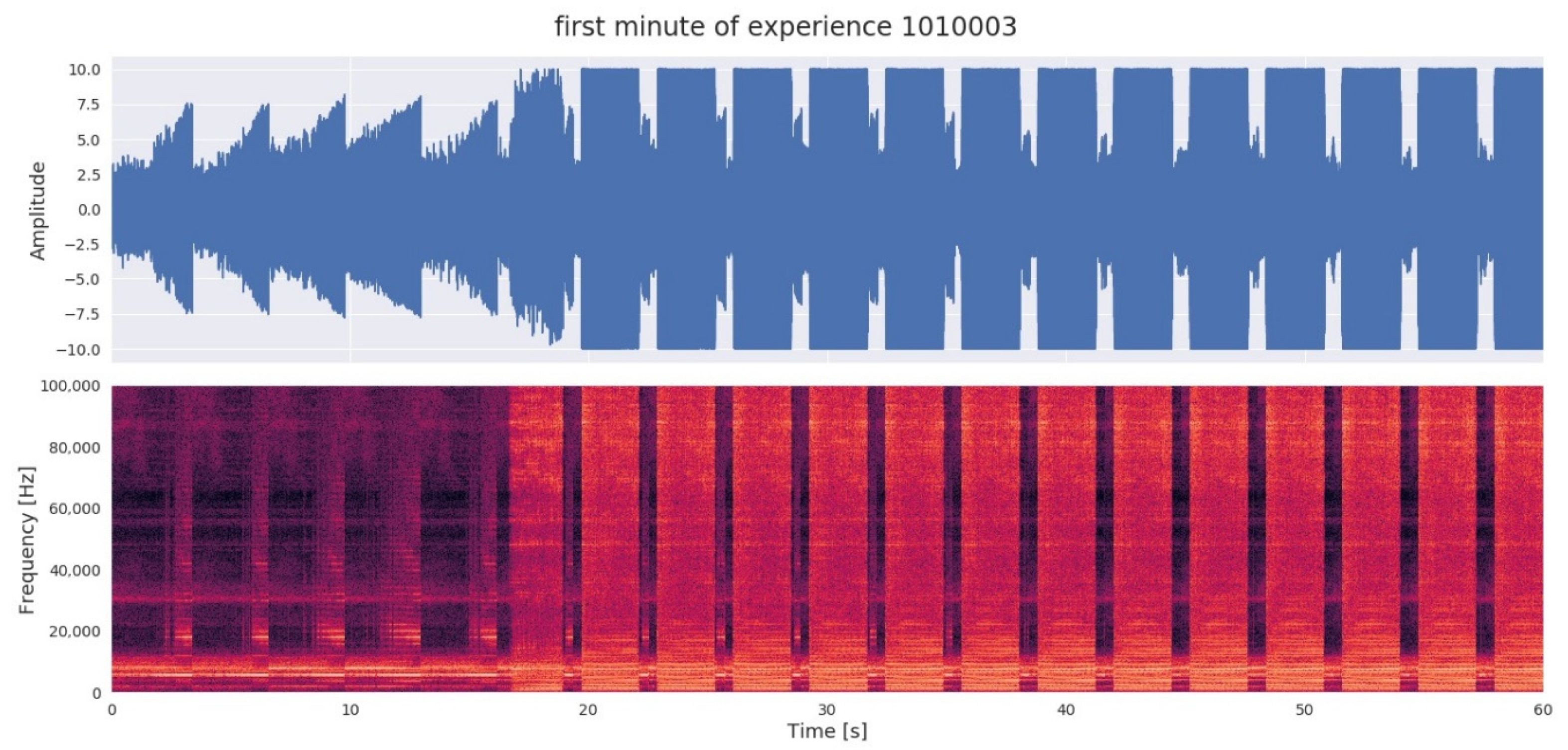
2.3. Milling Dataset
2.4. Labeling Approach
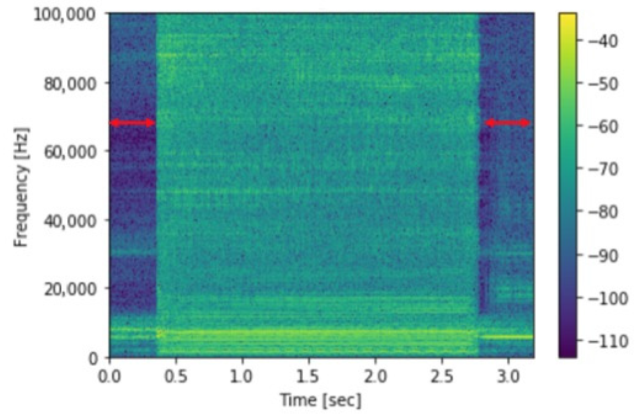
2.5. Feature Extraction
2.6. Classification
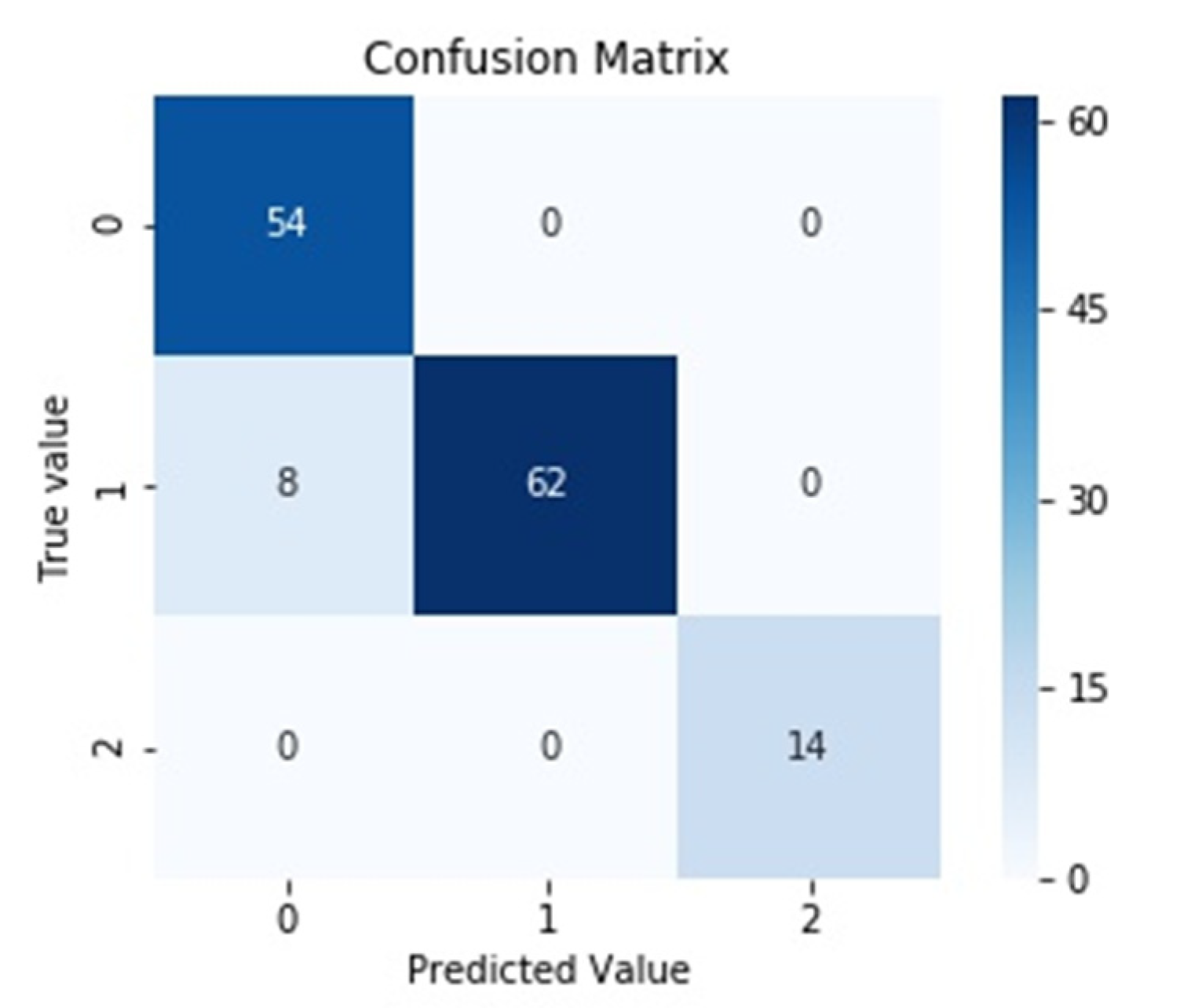
3. Results
4. Discussion
- Additional machines to assess the quality can be removed from the production line.
- If the quality estimation can be performed on the fly during the machining, tool breakage and material and time wastage can be avoided.
- The small dataset.
- The fact that realized milling process is simple, as it consists of linear passes repeated at different heights. More complex cutting operations can generate noise that could be more difficult to analyze.
- Only one type of material was used, along with one type of tool and one type of lubrication (no lubrication).
Author Contributions
Funding
Acknowledgments
Conflicts of Interest
Appendix A

| Layer (Type) | Output Shape | Param # |
|---|---|---|
| Conv2D (relu) | (None, 126, 126, 32) | 320 |
| Conv2D (relu) | (None, 124, 124, 64) | 18496 |
| MaxPooling2D | (None, 62, 62, 64) | |
| Dropout | (None, 62, 62, 64) | |
| Flatten | (None, 246016) | |
| Dense | (None, 128) | 31490176 |
| Dropout | (None, 128) | |
| Dense (softmax) | (None, 3) | 387 |
| Total params: 31,509,379 Trainable params: 31,509,379 Non-trainable params: 0 | ||
References
- Dou, J.; Xu, C.; Jiao, S.; Li, B.; Zhang, J.; Xu, X. An unsupervised online monitoring method for tool wear using a sparse auto-encoder. Int. J. Adv. Manuf. Technol. 2020, 106, 2493–2507. [Google Scholar] [CrossRef]
- Dornfeld, D.A.; Lee, Y.; Chang, A. Monitoring of Ultraprecision Machining Processes. Int. J. Adv. Manuf. Technol. 2003, 21, 571–578. [Google Scholar] [CrossRef]
- Shevchik, S.A.; Masinelli, G.; Kenel, C.; Leinenbach, C.; Wasmer, K. Deep Learning for In Situ and Real-Time Quality Monitoring in Additive Manufacturing Using Acoustic Emission. IEEE Trans. Ind. Inf. 2019, 15, 5194–5203. [Google Scholar] [CrossRef]
- Inasaki, I. Application of acoustic emission sensor for monitoring machining processes. Ultrasonics 1998, 36, 273–281. [Google Scholar] [CrossRef]
- Mouli, D.S.B.; Rameshkumar, K. Acoustic Emission-Based Grinding Wheel Condition Monitoring Using Decision Tree Machine Learning Classifiers. In Advances in Materials and Manufacturing Engineering; Li, L., Pratihar, D.K., Chakrabarty, S., Mishra, P.C., Eds.; Lecture Notes in Mechanical Engineering; Springer: Singapore, 2020; pp. 353–359. ISBN 9789811513060. [Google Scholar]
- Sachin Krishnan, P.; Rameshkumar, K. Grinding wheel condition prediction with discrete hidden Markov model using acoustic emission signature. Mater. Today Proc.
- Arun, A.; Rameshkumar, K.; Unnikrishnan, D.; Sumesh, A. Tool Condition Monitoring of Cylindrical Grinding Process Using Acoustic Emission Sensor. Mater. Today Proc. 2018, 5, 11888–11899. [Google Scholar] [CrossRef]
- Li, X. A brief review: Acoustic emission method for tool wear monitoring during turning. Int. J. Mach. Tools Manuf. 2002, 42, 157–165. [Google Scholar] [CrossRef]
- Ibarra-Zarate, D.; Alonso-Valerdi, L.M.; Chuya-Sumba, J.; Velarde-Valdez, S.; Siller, H.R. Prediction of Inconel 718 roughness with acoustic emission using convolutional neural network based regression. Int. J. Adv. Manuf. Technol. 2019, 105, 1609–1621. [Google Scholar] [CrossRef]
- Saeidi, F.; Shevchik, S.A.; Wasmer, K. Automatic detection of scuffing using acoustic emission. Tribol. Int. 2016, 94, 112–117. [Google Scholar] [CrossRef]
- Zhang, K.; Yuan, H.; Nie, P. A method for tool condition monitoring based on sensor fusion. J. Intell. Manuf. 2015, 26, 1011–1026. [Google Scholar] [CrossRef]
- Chung, K.T.; Geddam, A. A multi-sensor approach to the monitoring of end milling operations. J. Mater. Process. Technol. 2003, 139, 15–20. [Google Scholar] [CrossRef]
- Cao, X.; Chen, B.; Yao, B.; Zhuang, S. An Intelligent Milling Tool Wear Monitoring Methodology Based on Convolutional Neural Network with Derived Wavelet Frames Coefficient. Appl. Sci. 2019, 9, 3912. [Google Scholar] [CrossRef]
- Krishnakumar, P.; Rameshkumar, K.; Ramachandran, K.I. Tool Wear Condition Prediction Using Vibration Signals in High Speed Machining (HSM) of Titanium (Ti-6Al-4V) Alloy. Procedia Comput. Sci. 2015, 50, 270–275. [Google Scholar] [CrossRef]
- Luiz Lara Oliveira, T.; Zitoune, R.; Ancelotti, A.C., Jr.; Cunha, S.S., Jr. da Smart machining: Monitoring of CFRP milling using AE and IR. Compos. Struct. 2020, 249, 112611. [Google Scholar] [CrossRef]
- Xu, K.; Li, Y.; Liu, C.; Liu, X.; Hao, X.; Gao, J.; Maropoulos, P.G. Advanced Data Collection and Analysis in Data-Driven Manufacturing Process. Chin. J. Mech. Eng. 2020, 33, 43. [Google Scholar] [CrossRef]
- Krishnakumar, P.; Rameshkumar, K.; Ramachandran, K.I. Machine learning based tool condition classification using acoustic emission and vibration data in high speed milling process using wavelet features. IDT 2018, 12, 265–282. [Google Scholar] [CrossRef]
- Sachin Krishnan, P.; Rameshkumar, K.; Krishnakumar, P. Hidden Markov Modelling of High-Speed Milling (HSM) Process Using Acoustic Emission (AE) Signature for Predicting Tool Conditions. In Advances in Materials and Manufacturing Engineering; Li, L., Pratihar, D.K., Chakrabarty, S., Mishra, P.C., Eds.; Lecture Notes in Mechanical Engineering; Springer: Singapore, 2020; pp. 573–580. ISBN 9789811513060. [Google Scholar]
- Krizhevsky, A.; Sutskever, I.; Hinton, G.E. ImageNet Classification with Deep Convolutional Neural Networks. In Proceedings of the 25th International Conference on Neural Information Processing Systems-Volume 1; Curran Associates Inc.: Red Hook, NY, USA, 2012; pp. 1097–1105. [Google Scholar]
- Hawkins, D.M. The Problem of Overfitting. J. Chem. Inf. Comput. Sci. 2004, 44, 1–12. [Google Scholar] [CrossRef] [PubMed]
- Hripcsak, G. Agreement, the F-Measure, and Reliability in Information Retrieval. J. Am. Med Inform. Assoc. 2005, 12, 296–298. [Google Scholar] [CrossRef] [PubMed]


| Experience ID | Spindle Rotation Speed (Revolutions per Minute) | Number of Stairs Machined | Quality Label: 0 (Good), 1 (Intermediate), 2 (Bad) |
|---|---|---|---|
| 1 | 0 RPM | 0× | - |
| 2 | 29k RPM | 0× | - |
| 3 | 35k RPM | 0× | - |
| 4 | 29k RPM | 6× | 0, 0, 0, 1, 1, 1 |
| 5 | 33k RPM | 6× | 1, 1, 1, 1, 1 |
| 6 | 35k RPM | 3× | 1, 2, 2 |
Publisher’s Note: MDPI stays neutral with regard to jurisdictional claims in published maps and institutional affiliations. |
© 2020 by the authors. Licensee MDPI, Basel, Switzerland. This article is an open access article distributed under the terms and conditions of the Creative Commons Attribution (CC BY) license (https://creativecommons.org/licenses/by/4.0/).
Share and Cite
Carrino, S.; Guerne, J.; Dreyer, J.; Ghorbel, H.; Schorderet, A.; Montavon, R. Machining Quality Prediction Using Acoustic Sensors and Machine Learning. Proceedings 2020, 63, 31. https://0-doi-org.brum.beds.ac.uk/10.3390/proceedings2020063031
Carrino S, Guerne J, Dreyer J, Ghorbel H, Schorderet A, Montavon R. Machining Quality Prediction Using Acoustic Sensors and Machine Learning. Proceedings. 2020; 63(1):31. https://0-doi-org.brum.beds.ac.uk/10.3390/proceedings2020063031
Chicago/Turabian StyleCarrino, Stefano, Jonathan Guerne, Jonathan Dreyer, Hatem Ghorbel, Alain Schorderet, and Raphael Montavon. 2020. "Machining Quality Prediction Using Acoustic Sensors and Machine Learning" Proceedings 63, no. 1: 31. https://0-doi-org.brum.beds.ac.uk/10.3390/proceedings2020063031