Computational Fluid Dynamics Simulation to Predict the Airflow and Turbulence in a Wind Farm in Open Complex Terrain †


1
Department of Physics, Faculty of Science Tetouan, Abdelmalek Essaadi University, Tetouan 93 030, Morocco
2
Department TITM, National School of Applied Sciences at Tetouan, Abdelmalek Essaadi University, Tetouan 93 030, Morocco
*
Author to whom correspondence should be addressed.
†
Presented at the 14th International Conference on Interdisciplinarity in Engineering—INTER-ENG 2020, Târgu Mureș, Romania, 8–9 October 2020.
Proceedings 2020, 63(1), 33; https://0-doi-org.brum.beds.ac.uk/10.3390/proceedings2020063033
Published: 18 December 2020
(This article belongs to the Proceedings of The 14th International Conference on Interdisciplinarity in Engineering—INTER-ENG 2020)
Abstract
:The performance of a wind turbine depends on the characteristics of the airflow as well as the conditions of the atmospheric boundary layer (ABL). To evaluate accurately the amount of wind energy, it is required to have the exact height distribution of wind speed for the considered implementation site of a wind turbine. In this paper, computational fluid dynamics (CFD) simulation predictions provided by the standard k- turbulence model under neutral conditions were examined. The objective is to investigate the influence of hill slopes in the microscale wind farm on the airflow velocity to optimize the location of wind turbines. The results were validated by RUSHIL wind tunnel data and were compared with flat terrain.
1. Introduction
Wind energy is one of the most prominent renewable energy sources today. The increasing concerns with environmental issues are driving the search for more sustainable electrical sources. Wind energy along with solar energy, biomass, and wave energy is possible solutions for environmentally friendly energy production. The initialization of wind power installation, which started at the beginning of the 1980s, is very much related to the oil crises of the mid-1970s. During the 1980s, most wind power installations were limited to a few hundred kilowatts. The small size of those installations did not threaten the power system stability. The 1990s marked an important breakthrough in the industry. New concepts emerged because of the demand for more efficient power production and because of the necessity to comply with power quality requirements [1].
The production of wind energy potential for a given site often involves uncertainties due to the stochastic nature of wind speeds and the variation of the power curve [2]. Wind velocity distribution corresponds to the effect of airflow turbulent in the atmospheric boundary layer according to a complex pattern that depends hugely on associating peeling occurring on the airflow due to the roughness of the ground surface, local Reynolds number, and obstacles. It varies as a function of the altitude and the site topography. The wind farm performance affected by the presence of macroscopic obstacles on the surface of a plate modifies the flow characteristics of wind and the wind speed profile normal to that plate is changed. To evaluate the amount of wind energy, it is necessary to have the accurate height distribution of wind speeds on that location.
In this study, computational fluid dynamics (CFD) modeling is used to solve the turbulent airflow equations that consist of the Navier–Stokes equations coupled to the k- turbulence model and to simulate the turbulent flow over different slopes of the two-dimensional hills that are presented on the ground.
The major advantage of CFD is that it is a very compelling, non-intrusive, virtual modeling technique with powerful visualization capabilities, and engineers can evaluate the performance of a wide range of system configurations on the computer without the time, expense, and disruption required to make actual changes onsite; it has seen dramatic growth over the last several decades. This technology has widely been applied to various engineering applications such as automobile and aircraft design, weather science, civil engineering, and oceanography.
The main objective of this research is to perform a comprehensive CFD analysis in hilly terrain to optimize the siting of the turbines by considering their obstruction effect. While several studies have shown that complex terrain affects the wake flow of wind turbines [3,4,5], few research papers have focused on studying its effect on the velocity profile approaching the leading edge of the turbine, which may be an area for further research. Additionally, this work was carried out to assess the efficiency of the CFD model on the airflow distribution in the neutral atmospheric boundary layer (ABL) to describe the impact of topography in the micro-scale wind farms in open hilly terrain, which was considered by the implementation of four wind turbines aligned with two different hill slopes.
In this work, COMSOL Multiphysics software package [6] which is based on the Finite Element (FE) method was used to solve the fluid dynamics equations. This software allows to couple different equations in order to describe general Multiphysics phenomenon. Appropriate boundary layer conditions were applied. In the other hand, the precision of the standard k- turbulence model was examined by comparison with experimental data for the “Russian Hill” (RUSHIL) wind-tunnel study [7]. The velocity profile in different positions of the terrain are compared with those of flat plate without obstacle. The numerical results obtained show good agreement with experimental data. Thus, they indicate that the velocity profiles were highly affected by the presence of the hill, especially, on the steep slope.
2. Mathematical Formulation and Numerical Techniques
Choosing a particular CFD model mainly depends on the characteristics of the physical process to be simulated. It further depends on the goals of the numerical simulation and the available computational facilities. To achieve an accurate representation at the targeted turbulence scale, the whole comprehensive of the mathematical model was required. However, the computational cost is one of the important factors that should be taken into account.
In the present work, the Navier–Stokes equations coupled with the k- turbulence model in the case of the incompressible steady-state fluid flow are implemented by using COMSOL Multiphysics software package.
2.1. Reynolds-Averaged Navier–Stokes (RANS) Equations
The partial differential equations that present the average steady-state incompressible flow are described from continuity (Equation (1)) and momentum (Navier–Stokes) (Equation (2)), which simplifies to:
where v is the velocity, the density, p the pressure, F the density of volumetric forces acting in the fluid, and ∇ the gradient operator. is the dynamic viscosity that depends only on the physical properties of the fluid and is the turbulent eddy viscosity which is supposed to simulate unresolved velocity fluctuations .
The system of the equations has an additional term that means the turbulent Reynolds stress representing the influence of the fluctuation on the average flow. In order to close its system, this term must be determined. To achieve this condition, the standard turbulence model was chosen in the following section.
2.2. Standard Turbulence Model
The most common model used in CFD simulation for the turbulent applications is the standard turbulence model [8], which was introduced by [9]. The model solves for two transport equations, the turbulence kinetic energy k (Equation (3)); and the turbulence dissipation energy (Equation (4)), respectively [10]. The recommended values of standard closure constants implement in both of the transport equations given in Table 1. In the present work, these constants have been adjusted according to the features of the surface boundary layer in neutral atmospheric conditions suggested by [11].
2.3. Boundary Conditions
The full model to specify the turbulence airflow is mentioned above. The presence of the linear term in momentum equation produce some difficulty in the solving process of the equations. On the other hand, the hypothesis of the standard turbulence model is not applicable near the surface. However, an accurate specification of the boundary conditions on the various sides is needed. It is summarized in Table 2.
The boundary condition of the wall surface was fixed by scalable wall function condition that requires the standard turbulence model, which is presented in COMSOL Multiphysics by the following equations [12]:
- Velocity was applied as a no-slip condition
- Shear stress condition
with
- Turbulent kinetic energy and dissipation energy
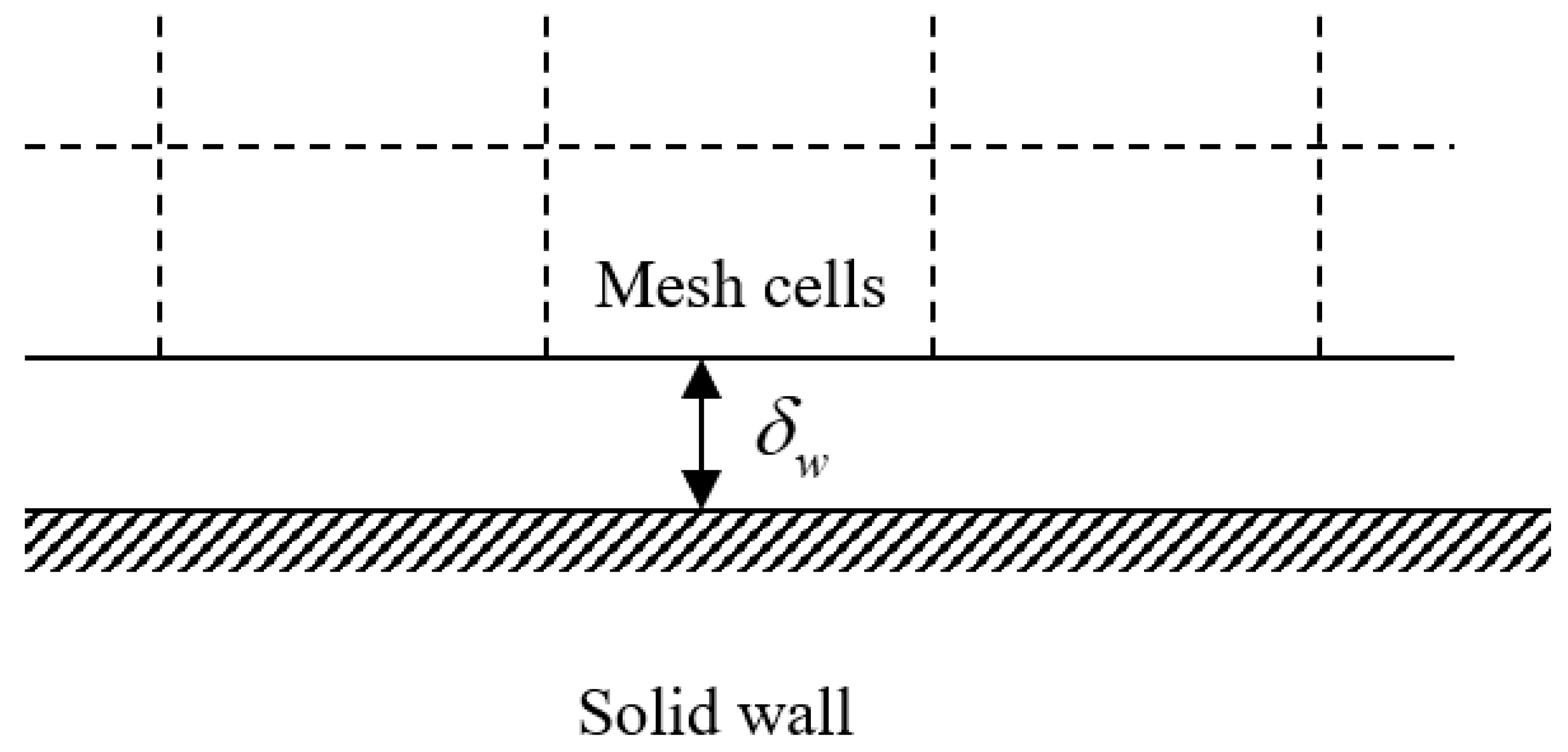
The scalable wall function is assumed to be positioned at a distance from the wall as shown in the Figure 1. This distance refers to the intersection of the logarithmic layer and viscous sublayer in the value of the dimensionless distance from equal to 11.06, where and is the friction velocity. The scalable wall function means that the dimensionless distance from the wall is limited from below so that it never become smaller than half of the height of the boundary mesh cell [6].
3. Computational Domain and Mesh Configuration
In this work, simulation was considered via a 2D airflow approximation of the problem. In addition, the implementation of four wind turbines aligned with two different hills slopes was performed. The wind turbines were separated by distances in x-direction such as x = −10D, x = 0D, x = 2D, x = 10D, respectively from the center of domain, where D = 125 mm is the rotor diameter and the hub height was yhub = 100 mm from y = 0.
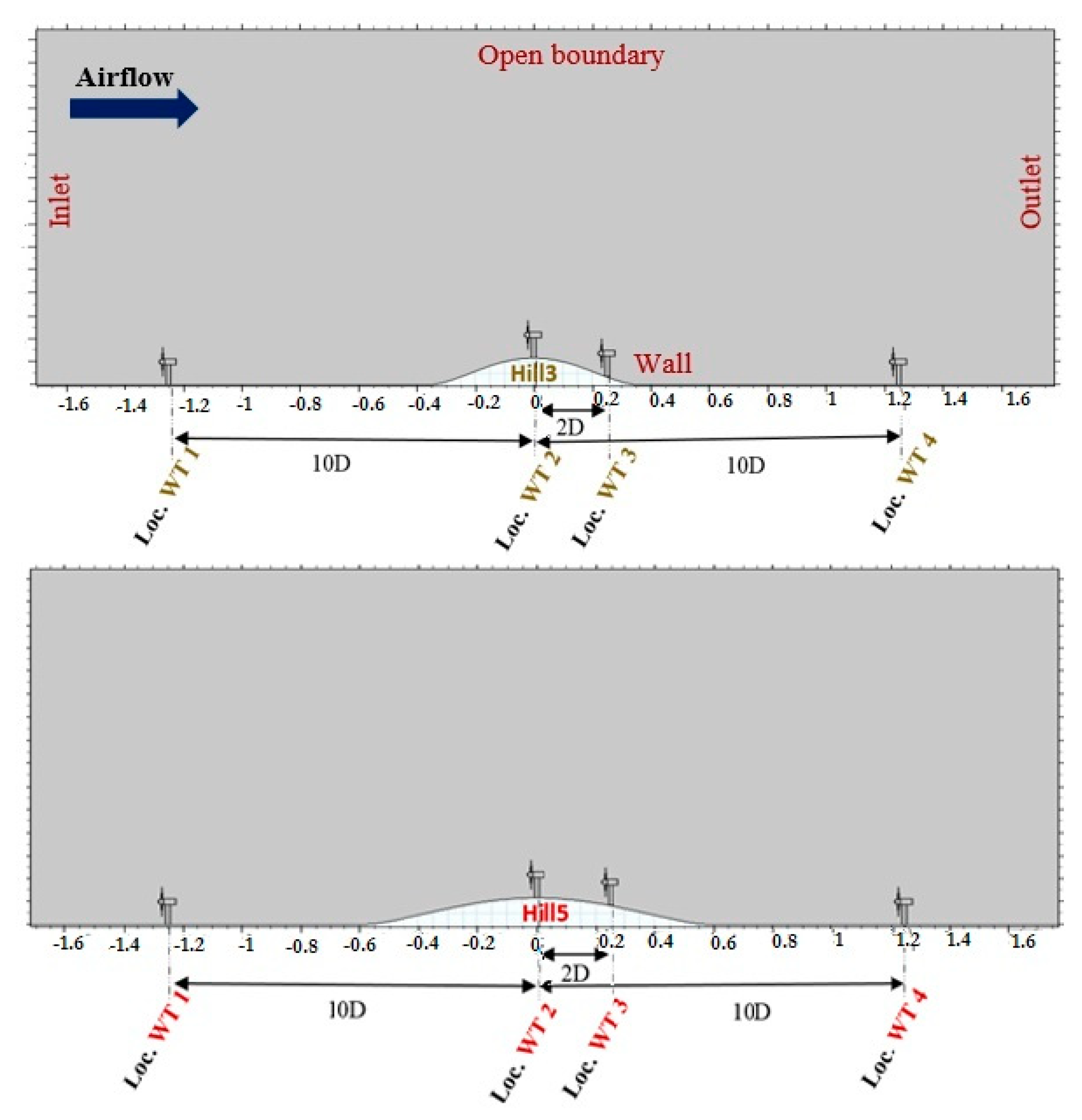
Assuming the wind tunnel data of the RUSHIL experiment [7], the computational domain was indicated as the same configuration mentioned in [13]. The surface is considered to be a horizontal plane with a hill as shown in Figure 2. The dimensions of the surrounding domain correspond to the length up and downstream of the top of the hill to vertical height of .
The slopes of the hills are defined by the parametric equation specified in [13]. They are called here Hill3 and Hill5 as function to their a/H ratios and according to their maximum hill slopes which are 26 and 16, respectively. The hill height H was fixed by 0.117 m. The uniform velocity and the friction velocity were fixed by and , respectively. On the other hand, the boundary layer depth takes a value equal to with a roughness length fixed by .
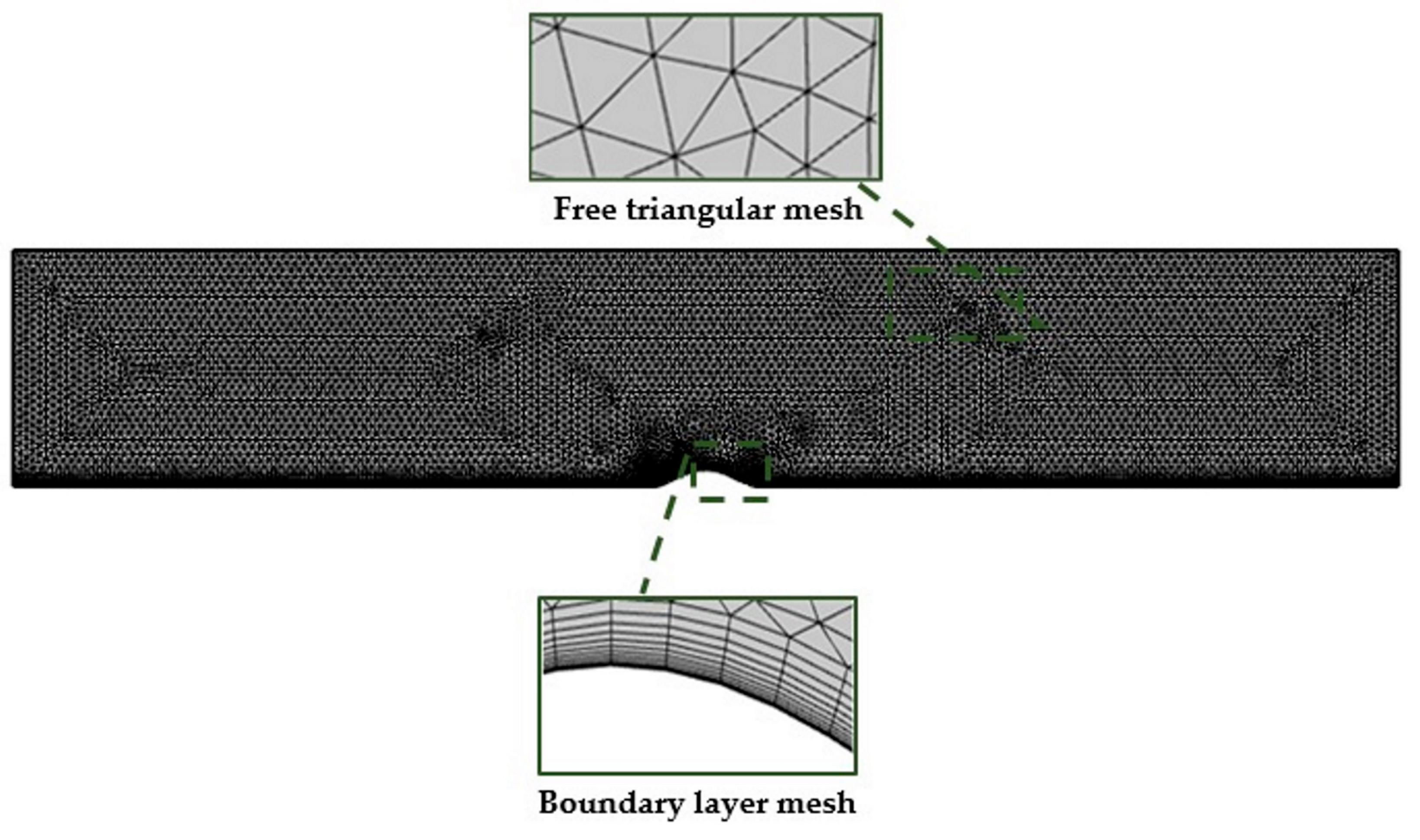
At the practical level, CFD simulation typically faces the challenge of creating an initial mesh that is sufficiently accurate to produce a solution for the real problem and in particular for the required wall law resolution. In this case, a parametric study was also performed in order to identify a suitable mesh. The ground surface was meshed using the properties of the boundary layer mesh, then, a free triangle mesh elements was used for the whole of the computational domain. The complete domain contains 15,065 mesh elements and it was definite with the maximum elements growth rate fixed at 1.2. The configuration of the obtained mesh until convergence was shown in Figure 3.
4. Results and Discussion
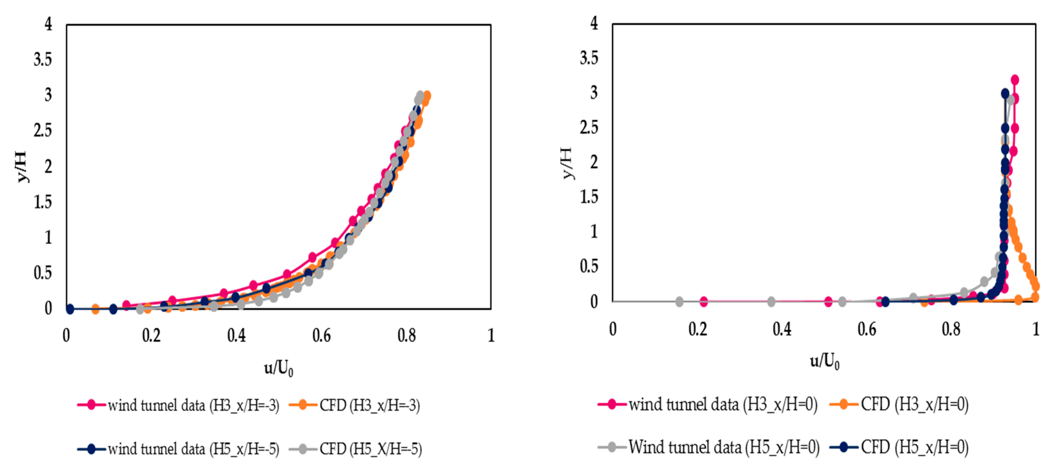
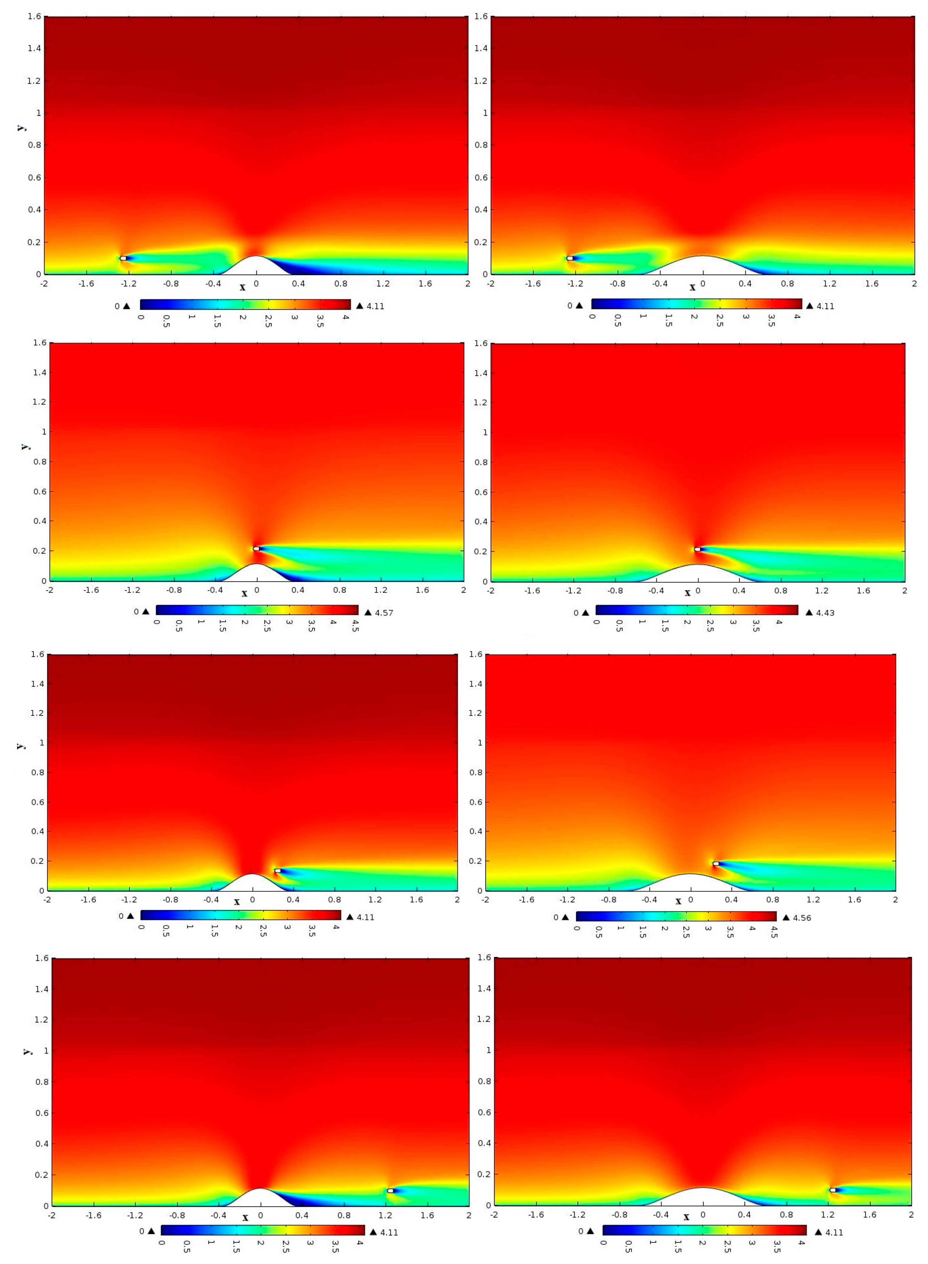
To study the surface flow over hilly terrain further, three cases are analyzed below. The first considers the streamwise velocity profile implementation in Figure 4, which show the agreement with wind tunnel data measurement. The third case considers the presence of the Hill3 and Hill5 with the installation of the wind turbines in several locations (hilly terrain + wind farm). First location at x = −10D in the upstream of both hills. Therefore, the second location is presented and placed on top of both hills (Hill3 and Hill 5) at x = 0D, while the third involves the turbine placed at x = 2D of both hills. Finally, the fourth contains the turbine placed far away from both hills and at distance x = 10D from the symmetry of the hills. Then, the streamwise velocity profile was measured at the hub height for four positions, as shown in Figure 5.
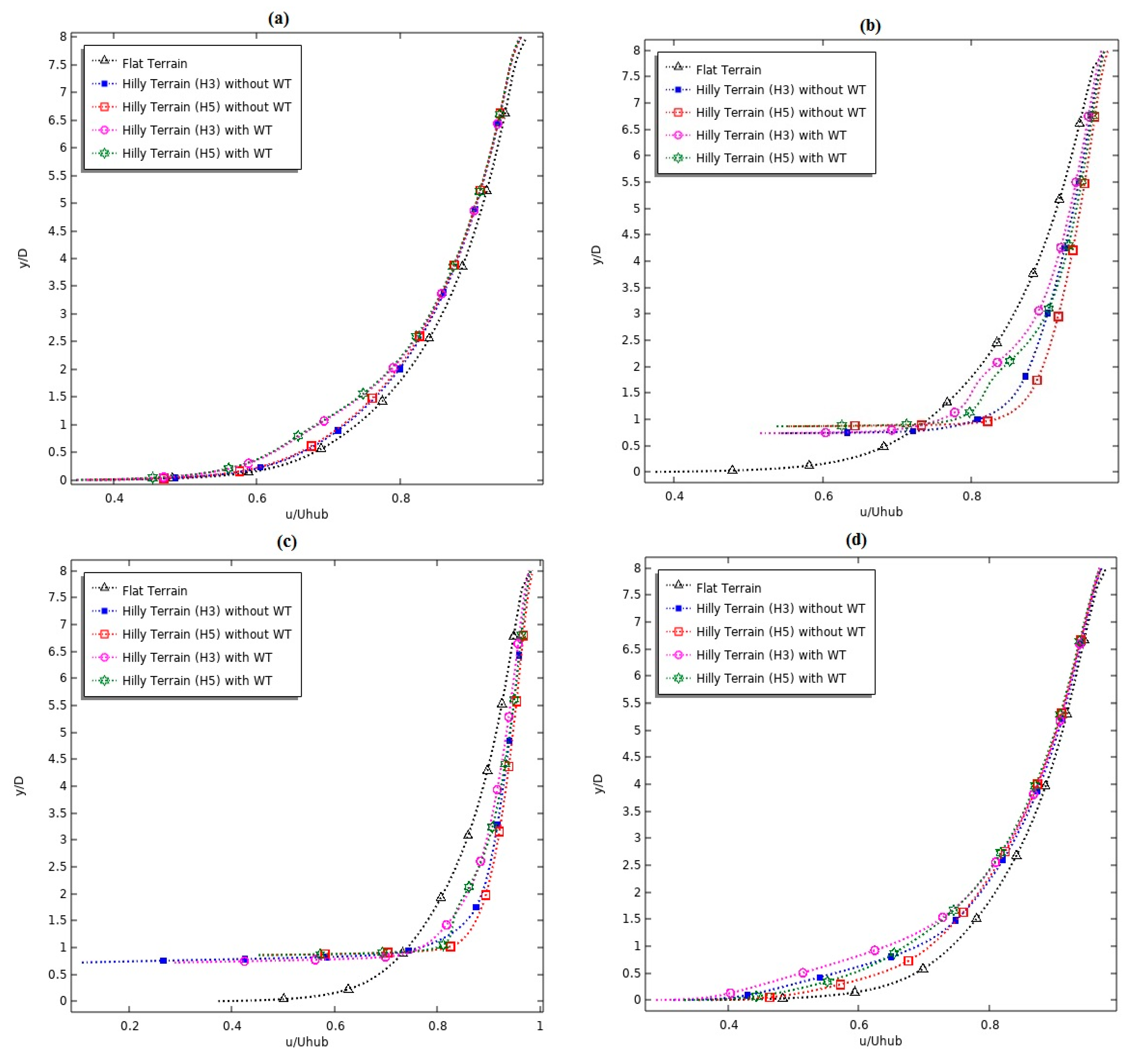
Further, to study the distribution of the flow over wind farm in complex terrain, the simulation was done at four selected locations, as illustrated in Figure 5. The mean streamwise velocity profiles for two cases (with and without wind turbines) around hilly terrain with various slope are schemed in Figure 6. The wind-speed curves of inflow on flat terrain are plotted too for comparison purposes. All the velocities presented in Figure 6 are normalized with hub height velocity Uhub. The wind-speed profile was taken at 1D before of the center of the wind turbines.
Figure 6a treats the horizontal stream-wise velocity along of the wind turbine for the Case 1, which is placed at the distance of −10D in the upstream of the hill. Firstly, it can be seen that under the hill height (y/D < 1), the velocity distribution on hilly terrain without wind turbine is depressed when compared with the upstream on flat plate. The little discrepancies between complex terrain without wind turbine and flat terrain from close the ground to the hill summit. Therefore, it is due to the blockage effect on the flow situated in lee side of the hill. Hence, it is necessary to consider this effect because it can decrease the extractable kinetic energy from the air by wind turbine.
Then, above (y/D > 1) the horizontal velocity increase with the elevation, these discrepancies reduce continuously and finally disappear after the top of the hill. Thus, if the wind turbine moves by the distance higher than 10D, it can decrease this blockage effect. On the other hand, the important difference of stream-wise velocity distributions on x-y planes of hilly terrain with wind turbine can be seen when compared with hilly terrain without wind turbine. However, this difference is caused by obstruction of the wind turbine. Consequently, in order to ensure noble studies and results as assessment of wind farms, all these effects cannot be ignored.
Case 2 describes the behavior of the flow on the crest of the hill, with the wind turbine placed at this location.
In this section, the position is analyzed of horizontal-spanwise curves of the normalized averaged streamwise velocity on the top hill for the both of the hill slopes. It can be observed from Figure 6b, that when the cut-line is placed at 1D before center of wind turbine, the effect of the acceleration on the hill was clearly presented. An interesting observation that might be drawn from Figure 6b, is that the maximum speed is on the top of the hill for H3 and H5 without installed wind turbine due to the compression on this location depending on the wind side and leeward slope of the hill and the influence of change distribution of the flow caused by different positions at all of the length hill. Then, we can observe the increase of velocity from the hill height to the hub height (0.73 < y/D < 2) for H3 and (0.86 < y/D < 2) for H5 when compared by flat terrain y/D = 0 (u/Uhub = 0.78). However, the velocity for high slope H3 reaches the value of u/Uhub = 0.87 and u/Uhub = 0.9 for low slope H5. Therefore, the local acceleration of the hilly terrain can reproduce the increase of power ratio in wind farms and adjust the distribution of the wind speed to decrease the fatigue loads acting on the wind turbine. On the other hand, when installing the wind turbine on the top of the both of hill, it can be seen from Figure 5 (line 2) the distribution of velocity and from Figure 6b the streamwise velocity curves for Hill3 and Hill5 by the presence of wind turbine are lower than complex terrain without turbine, especially when compared with the velocity from the hill height until upper limit of the wind turbine rotor (0.73 < y/D < 2.25 for H3 and 0.86 < y/D < 2.25 for H5). Thus, the difference for the H3 high slope is about 2.5% and for the H5 low slope is about 3.5%. Then, the speed-up surface is choked by the presence of nacelle and the hub in our computational domain, that is to say, the presence of wind turbine in reality. In other way, it can be positive for increased lifetime of the rotor blades.
Figure 6c gives the horizontal velocity profile for case 3 in which wind turbine is installed at downside of the hill (2D at the down of the hill). It is based on the comparison of five curves, which include the two hilly terrains for the high and low slope H3 and H5, respectively, with and without wind turbine and the curve of flat terrain. The important effect of the slope hill can clearly be observed over downhill in Figure 5a and in wind profile of H3 and H5 presented in Figure 5c for hilly terrain without wind turbine that the high slope produce steep detachment and separation of the boundary layer compared to that of the low slope. However, its steep detachment and separation produce the strong adverse pressure gradient in this region, which contributes to the large decreasing of wind speed, so that the wind turbine cannot extract a significant quantity of kinetic energy. In addition, the rotor blades can be affected by the reversed flow in the developed recirculation region at downwind of the obstacle. The two other wind profiles show the distribution of velocity of H3 and H5 with location wind turbine. At this point, the little decrease of velocity for the range 0.9 < y/D < 2 can be shown due to the obstructing wind turbine that increases the adverse pressure gradient leeward of the obstacle. In addition, the velocity of the high slope H3 at this position is lower than H5 due to the difference steep of the separation. Furthermore, the uniform distribution of velocity continued in this location due to the previous effect of acceleration on the crest of the hill.
Comparison of wind-speed curves at a distance 10D far from the hill for flat terrain and hilly terrain for both hills with the absence of wind turbine, and speed curves at the similar location with wind turbine is plotted in Figure 6d. Whereas, as mentioned above, the velocity with turbine is lower than the absence of the wind turbine, it can see from Figure 6d that there are little discrepancies between the two cases, therefore its effects on the rotating blades can be ignored. However, the effect that cannot be neglected is the decrease of velocity that is shown clearly in Figure 6d when compared with flat terrain. Its thrust is such that the velocity profile returns to take original form of the atmospheric boundary layer profile, but the impact of the hill largely degrades the wind speed. The slope of hill affects the developing of the scale of separation, which can be seen from the Figure 5 (line 4) and Figure 6d the wind turbine in the case 4 affect by the large separation of the H3 hill by comparison with H5. Moreover, the large separation can produce the increase of turbulence intensity, which increases the fluctuations loads acting on the blades of wind turbine. To reduce the most significant impact on results and to increase the power ratio in this location, it would be necessary to adjust the distance between hill and installed wind turbine.
The results show that the presence of the hills in wind farm have a positive influence on the performance of the wind-turbine, but then again, it would be necessary to take account the change of velocity results in the implementation of the wind turbine for the given respectable conditions of micro-siting. On the other hand, choosing the location that contribute significantly the increase of the lifetime of the wind turbines is important.
5. Conclusions
A CFD simulation was proposed and applied to examine the impact of micro-scale wind turbines on wind farms within both flat and hilly configurations, on two different slopes in this study. However, it was based on the simulation of the implementation of four various positions of the wind turbine. The changes and distributions of wind speed were discussed. The main findings of this study can be summarized as follows:
- Hill slopes are an important element for flow characteristics and disturbing effect. The steep slope and the separation of the flow due to the high adverse pressure gradient will considerably decrease the average speed.
- The velocity distribution of modelling the wind turbine in the simulation process is more likely than for the absence of the wind turbine.
- In the crest of the hill, the average speed on two positions highly increases, which leads to an extractable maximum power rate. In addition, reduced fatigue loads, which act on wind turbines on the crest of hill caused by the decrease in turbulence at these locations, yield to increase the lifetime of the rotor blade.
- The velocity profile in the wind turbine located at the down of the hill is still higher for low slope due to the small effect of the separation than the high slope. Therefore, the wind speed profile returns to the form of the boundary layer profile for both cases before and after the hill. The velocity of a wind turbine located at some distance before and after the hill is even lower than that of flat terrain due to the separation and interaction airflow effect in the windward side, which can be caused by choosing a small distance.
On another hand, for the accuracy of siting of the wind farms, the accurate study of the affecting the two lateral of the hill, the increase of turbulence, the characteristics of the flow affected by the change topography and obscurity of the implement wind turbines should be considered. Nevertheless, the numerical solutions achieved indicate that the wind farm siting in the hilly ground is appropriate.
Conflicts of Interest
The authors declare no conflict of interest.
References
- Bhattacharya, P. Wind Energy Management; Smiljanic, T., Ed.; IntechOpen: Rijeka, Croatia, 2011; ISBN 9533073365. [Google Scholar]
- Jin, T.; Tian, Z. Uncertainty analysis for wind energy production with dynamic power curves. In Proceedings of the 2010 IEEE 11th International Conference on Probabilistic Methods Applied to Power Systems, Singapore, 14–17 June 2010; IEEE: New York, NY, USA, 2010; pp. 745–750. [Google Scholar]
- Alfredsson, P.H.; Segalini, A. Introduction Wind farms in complex terrains: An introduction. Philos. Trans. A Math. Phys. Eng. Sci. 2017, 375. [Google Scholar] [CrossRef] [PubMed]
- Choudhry, A.; Mo, J.-O.; Arjomandi, M.; Kelso, R. Effects of Wake Interaction on Downstream Wind Turbines. Wind Eng. 2014, 38, 535–547. [Google Scholar] [CrossRef]
- Yan, S.; Shi, S.; Chen, X.; Wang, X.; Mao, L.; Liu, X. Numerical simulations of flow interactions between steep hill terrain and large scale wind turbine. Energy 2018, 151, 740–747. [Google Scholar] [CrossRef]
- COMSOL Multiphysics. Introduction to COMSOL Multiphysics; COMSOL Inc.: Stockholm, Sweden, 2016. [Google Scholar]
- Khurshudyan, L.H.; Snyder, W.H.; Nekrasov, I.V. (Eds.) Flow and Dispersion of Pollutants over Two-Dimensional Hills: Summary Report on Joint Soviet-American Study; Version Details—Trove; Environmental Protection Agency: Washington, DC, USA, 1982. [Google Scholar]
- Pope, S.B. Turbulent Flows; Cambridge University Press: Cambridge, UK, 2000; ISBN 9780511840531. [Google Scholar]
- Jones, W.; Launder, B. The prediction of laminarization with a two-equation model of turbulence. Int. J. Heat Mass Transf. 1972, 15, 301–314. [Google Scholar] [CrossRef]
- Ferziger, J.H.; Peric, M. Computational Methods for Fluid Dynamics, 3rd ed.; Springer: Stanfrod, CA, USA, 2002. [Google Scholar]
- Panofsky, H.A.; Dutton, J.A. Atmospheric Turbulence. Models and Methods for Engineering Applications, 1st ed.; John Wiley & Sons: New York, NY, USA, 1984. [Google Scholar]
- COMSOL Multiphysics. Multiphysics COMSOL Modeling Guide; COMSOL Inc.: Stockholm, Sweden, 2007; ISBN 1781273332. [Google Scholar]
- Castro, I.P.; Apsley, D.D. Flow and dispersion over topography: A comparison between numerical and laboratory data for two-dimensional flows. Atmos. Environ. 1997, 31, 839–850. [Google Scholar] [CrossRef]
Figure 1.
Distance from the wall to the computational domain.

Figure 2.
Schematic of the computational domain: (Top) Hill3+ Wind farm, (Bottom) Hill5+ Wind farm.

Figure 3.
Detail of the mesh elaborated with free triangle elements and the boundary layer mesh near the ground surface.
Figure 3.
Detail of the mesh elaborated with free triangle elements and the boundary layer mesh near the ground surface.

Figure 4.
Mean streamwise profiles of velocity component: (left) Hill3+ Hill5+ Wind tunnel data (upstream x/H = −3 for H3 and x/H = −5 for H5), (right) Hill3+ Hill5+ Wind tunnel data (summit x/H = 0).
Figure 4.
Mean streamwise profiles of velocity component: (left) Hill3+ Hill5+ Wind tunnel data (upstream x/H = −3 for H3 and x/H = −5 for H5), (right) Hill3+ Hill5+ Wind tunnel data (summit x/H = 0).

Figure 5.
Contours of average velocity in the x-y direction for four location of wind turbine with two slopes of the hills (H3 and H5): (line 1) x = −10D, (line 2) x = 0D, (line 3) x = 2D, (line 4) x = 10D.
Figure 5.
Contours of average velocity in the x-y direction for four location of wind turbine with two slopes of the hills (H3 and H5): (line 1) x = −10D, (line 2) x = 0D, (line 3) x = 2D, (line 4) x = 10D.

Figure 6.
Comparison of the normalized mean streamwise of velocity component for four location of wind turbine with two slopes of the hills (H3 and H5): (a) x = −10D (cut-line at 1D before center of WT); (b) x = 0D (cut-line at 1D before center of WT); (c) x = 2D (cut-line at 1D before center of WT); (d) x = 10D (cut-line at 1D before center of WT).


Table 1.
Overview of the closure constants used for the standard turbulence model.
| Standard | 0.09 | 1.44 | 1.92 | 1.0 | 1.3 | 0.41 |
| Neutral ABL | 0.033 | 1.176 | 1.92 | 1.0 | 1.3 | 0.42 |
Table 2.
Summary of the boundary conditions.
| Boundary Conditions | Inlet | Outlet | Wall | Open Boundary |
|---|---|---|---|---|
| Standard | | Scalable Wall function |
Publisher’s Note: MDPI stays neutral with regard to jurisdictional claims in published maps and institutional affiliations. |
© 2020 by the authors. Licensee MDPI, Basel, Switzerland. This article is an open access article distributed under the terms and conditions of the Creative Commons Attribution (CC BY) license (https://creativecommons.org/licenses/by/4.0/).
Share and Cite
MDPI and ACS Style
Narjisse, A.; Khamlichi, A. Computational Fluid Dynamics Simulation to Predict the Airflow and Turbulence in a Wind Farm in Open Complex Terrain. Proceedings 2020, 63, 33. https://0-doi-org.brum.beds.ac.uk/10.3390/proceedings2020063033
AMA Style
Narjisse A, Khamlichi A. Computational Fluid Dynamics Simulation to Predict the Airflow and Turbulence in a Wind Farm in Open Complex Terrain. Proceedings. 2020; 63(1):33. https://0-doi-org.brum.beds.ac.uk/10.3390/proceedings2020063033
Chicago/Turabian StyleNarjisse, Amahjour, and Abdellatif Khamlichi. 2020. "Computational Fluid Dynamics Simulation to Predict the Airflow and Turbulence in a Wind Farm in Open Complex Terrain" Proceedings 63, no. 1: 33. https://0-doi-org.brum.beds.ac.uk/10.3390/proceedings2020063033