Control Strategies for Thermal Processes in Chemical Industry †

Department of Electrical Engineering and Information Technology, George Emil Palade University of Medicine, Pharmacy, Science, and Technology of Târgu Mureș, Gh. Marinescu Street, No. 38, 540139 Târgu Mureș, Romania
†
Presented at the 14th International Conference on Interdisciplinarity in Engineering—INTER-ENG 2020, Târgu Mureș, Romania, 8–9 October 2020.
Proceedings 2020, 63(1), 34; https://0-doi-org.brum.beds.ac.uk/10.3390/proceedings2020063034
Published: 18 December 2020
(This article belongs to the Proceedings of The 14th International Conference on Interdisciplinarity in Engineering—INTER-ENG 2020)
Abstract
:In the current context, the control of the industrial processes continues to be very important, due to the rapid modification of the economic conditions, the development of production and the tightening of environmental and safety conditions. This paper presents the technological scheme for obtaining the saturated steam from superheated steam and proposes Proportional–Integral-Derivative (PID) controller options based on an internal model, Integral of Time Multiplied by Absolute Error (ITAE) criterion and Ziegler–Nichols criterion. The simulation tests are performed using the Matlab software.
1. Introduction
Due to the existence of an important chemical factory in the Mureș industrial area, the students and the academic staff have the opportunity to carry out technological installation studies and test the control possibilities for processes with parameters such as: temperature, level, pressure, flow, pH etc.
Additionally, the chemical engineers require technical knowledge and tools to facilitate their work in modern technological installations.
Thus, the use of well-defined mathematical modeling methods and advanced monitoring systems for the industrial process allows high performance analysis. Moreover, an advanced approach involves the understanding of the dynamic regimes and the feedback and stability concepts used in control systems analysis.
Such topics are addressed by the specialists in the field of control systems in collaboration with technological and chemical engineers.
Thus, the mathematical modeling principles for the first-order and high-order systems, the closed-loop control mechanisms, as well as the tuning techniques for Proportional–Integral-Derivative (PID) controllers, are developed with significant examples in [1,2].
The mathematical modeling of processes with flow, level, pressure, temperature control, and the control loops for these parameters is detailed in [3]. In [4], simple and advanced techniques for choosing and tuning of the PID controllers are presented, including the method based on the internal model.
In [5], the implementation results of an internal model control (IMC), with set-point tracking, for flow control applications are presented. An internal model control for unstable processes, based on a standard IMC, is proposed in [6], while [7] presents an IMC system for level control applications implemented for two interconnected tanks.
An IMC structure for a Multi-Input Multi-Output (MIMO) system, which simultaneously ensures the decoupling and rejection of the disturbance, is developed in [8]. The sensitivity analysis with IMC PID controllers, based on the Nyquist stability criterion, is detailed in [9].
The IMC procedure for Single-Input Single-Output (SISO) systems, which leads to PID controllers and to variants for nonlinear systems, is detailed in [10,11]. Other tuning algorithms and tuning techniques are suggestively presented in [12]. The control strategies study can be performed using dedicated programs and environments, such as Matlab. Significant usage examples are those in [13].
This paper aims to analyze, using simulation, the behavior of a technological installation that produces saturated steam from superheated steam, with various PID control structures. Section 2 presents the mathematical modeling of a thermal process, and Section 3 details the practical schema of the steam temperature control in a chemical saturator and the equivalent block diagrams in which the transfer functions are highlighted. The control principles based on the internal model and the tuning relations for the automatic controller are detailed in Section 4. The behavior of the process with IMC, Integral of Time Multiplied by Absolute Error (ITAE) and Ziegler–Nichols controllers is presented in Section 5, followed by conclusions regarding the obtained performances (Section 6).
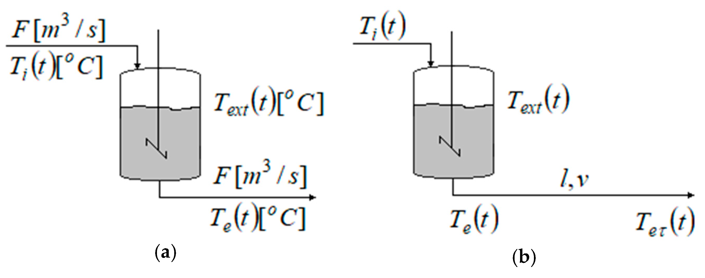
2. Mathematical Modeling of a Thermal Process
This is considered the thermal system consisting of a tank with a product which has the input parameters: F, Ti. The following situations are considered for the output [1,2,3]:
The mathematical modeling involves determining the relationship between the outlet temperature, Te(t) and the inlet temperature, Ti(t), considering that there is a heat exchange between the tank and the environment.
The dynamic equation has the following form:
where: is the volumetric flow ; —the input/output density of the fluid ; —the input/output enthalpy of the fluid ; —the heat exchange with the environment; V—the volume ; —the internal energy of the fluid .
Considering the constant pressure, in terms of temperature, it results in:
where: are the input/output temperatures of the fluid/product ; —the input/output caloric capacity (at constant pressure) ; —the specific heat (at constant volume) ; —the thermal transfer coefficient (constant); A—the thermal transfer area ; —the environment temperature .
For the control strategy, the steady state relation: is considered and the following infinitesimal variations are defined:
The dynamic equation becomes:
where: is the time constant [sec.]; —non-dimensional constants.
Any change in the values will affect the value of the time constant T and will be seen in the response speed.
Based on the Laplace transformation, it results in:
If the external temperature variation is , it results in: , and if , it results in: , with ; , which means that the Ti signal influences Te much more than Text does.
If the output product passes through a pipe section, the mathematical model is augmented with the transport time (time delay), , as follows:
respectively:
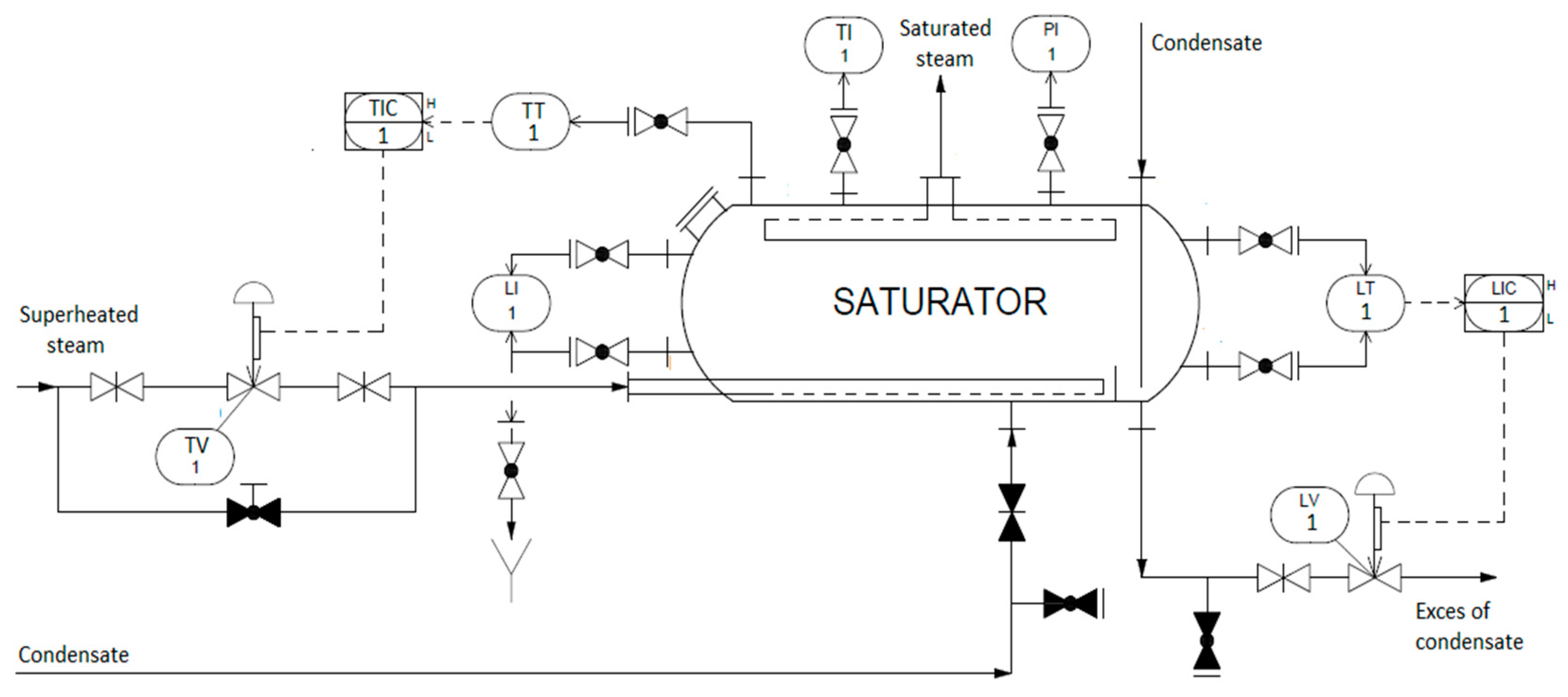
3. Temperature Control Diagram
The practical control diagram (Figure 2) involves the measurement and transmission of the product’s output temperature (TT—temperature transmitter), processing this information according to the control law (TIC—temperature controller) and generating the command signal to the actuator (TV—temperature valve). In addition, the installation is provided with temperature, pressure and level indicators (TI, PI, LI) and with a level control loop (LT, LIC, LV) [1,2,4,5,6,7,8,9,10,14].
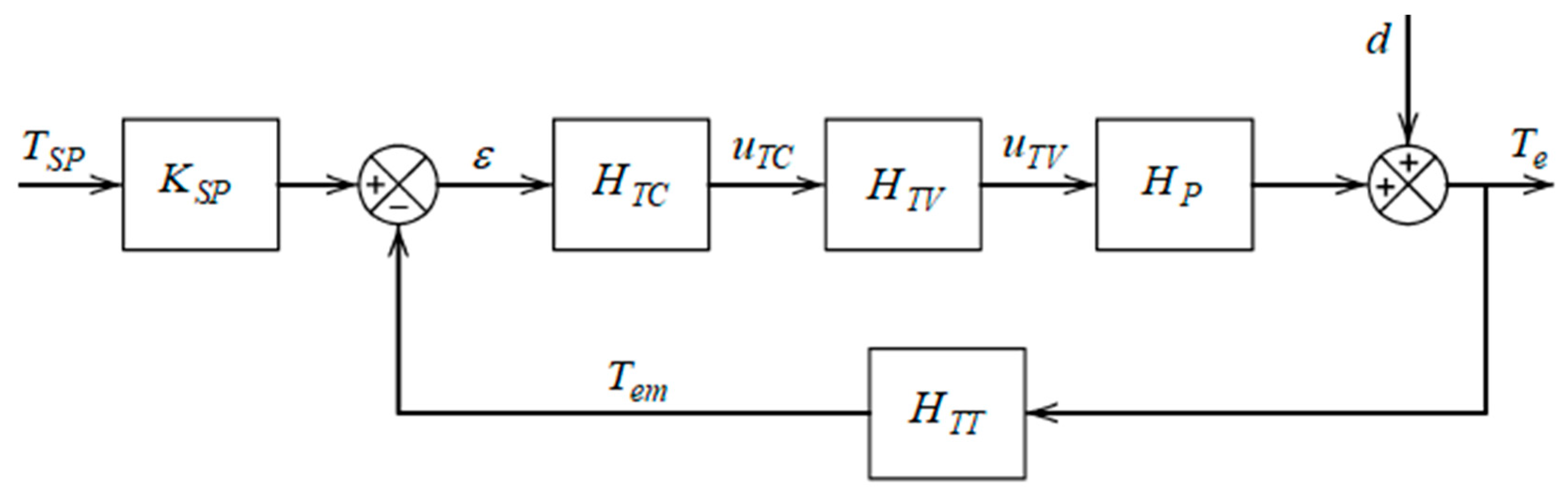
The associated block diagram highlights the transfer functions for: —controller; —actuator; —process with delay time; —temperature transducer/sensor; —gain on the set-point path and the signals ; —set-point and output temperatures; —error; —command; —manipulation signal; —disturbance (Figure 3).
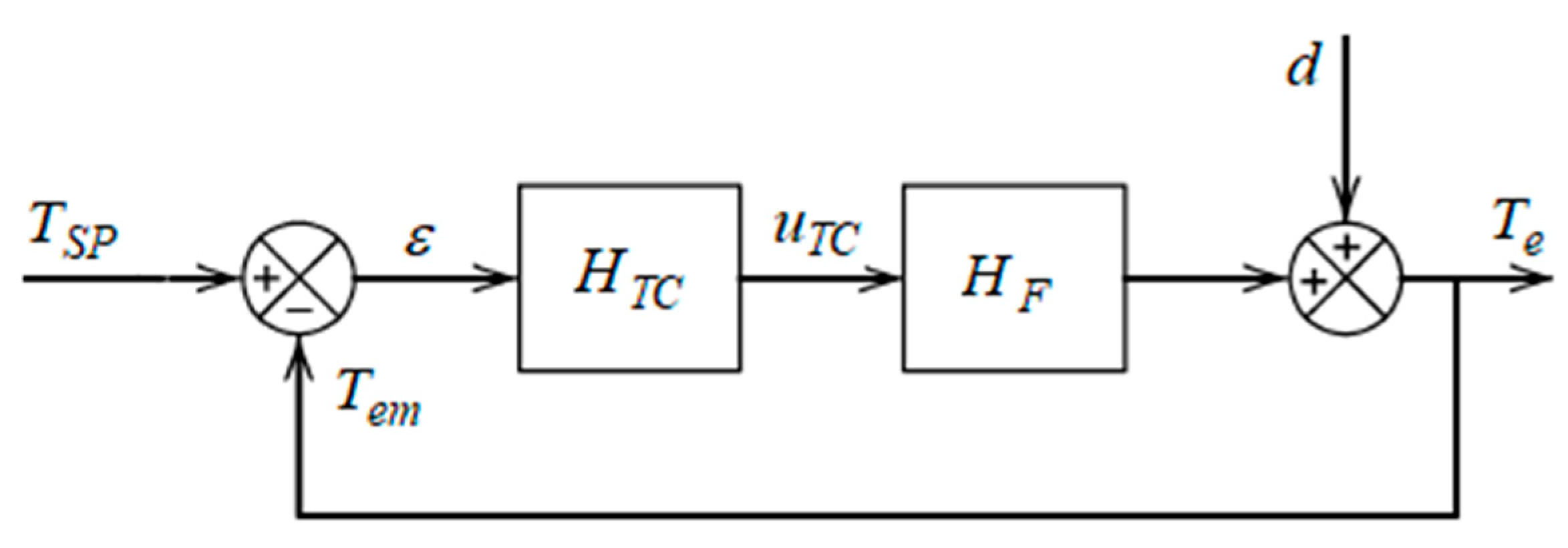
The closed-loop transfer function is:
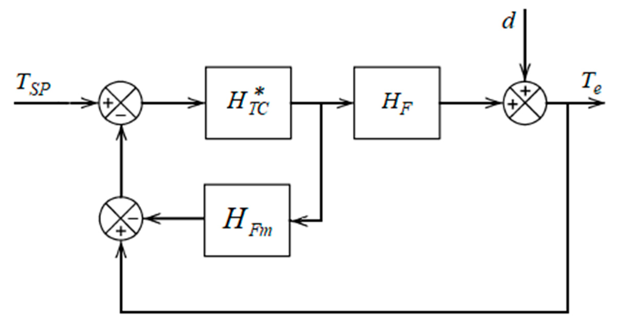
considering the hypothesis: și (Figure 4).
4. Design of the IMC Controller
A control solution takes into consideration the uncertainties which affect the process and involves determining the controller’s structure based on the internal model (IMC) of the process, (Figure 5) [10,11].
The conventional control diagram (Figure 4) and the IMC diagram (Figure 5) are equivalent if the controllers and meet the following condition:
In order to determine the IMC controller:
− the process model, is factored:
where: contains the time delay and the zeros situated in the right half of the complex plane;
− the IMC controller is designed as:
where:
is a low-pass filter, which reduces the sensitivity of the control system to modeling errors; is a design parameter.
Considering the transfer function of the process:
designing the IMC controller depends on the approximation expression of the time delay.
If , meaning that the model and the process model are identical and the Pade approximation is used as:
after replacing it in relationship (17), it results in:
The transfer function of the controller (15) becomes:
and the equivalent controller (13) has the form:
with the PID standard expression:
where the tuning parameters are:
If the Taylor approximation is used:
the transfer function of the PI controllers is:
where the tuning parameters are:
5. Experimental Results and Discussions
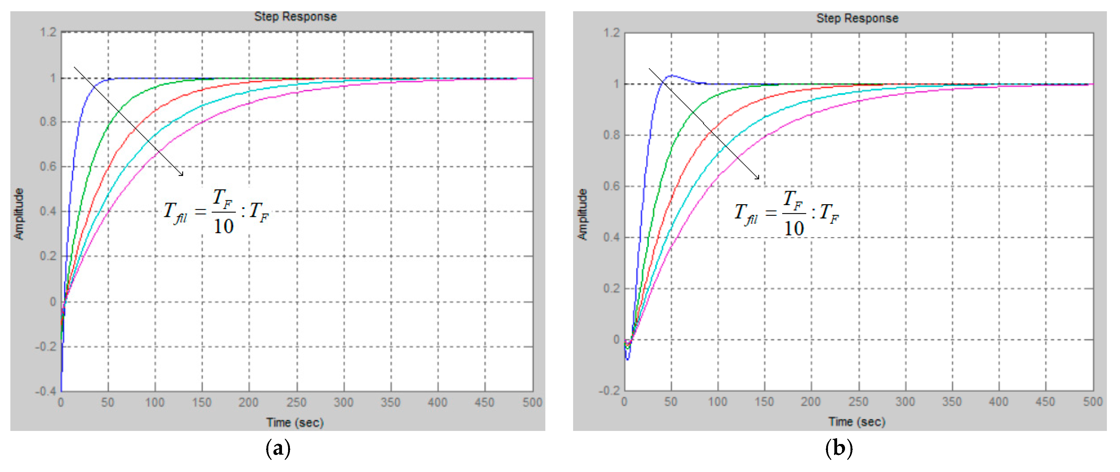
Considering the practical diagram implemented for the temperature control (Figure 2) with the transfer function: , different control structures were determined and the performances were analyzed. Thus, with a PID controller (22) and the tuning parameters described by (23), respectively, with a Proportional–Integral (PI) controller (25) and the tuning parameters (26), the indicial responses in Figure 6 were obtained [13].
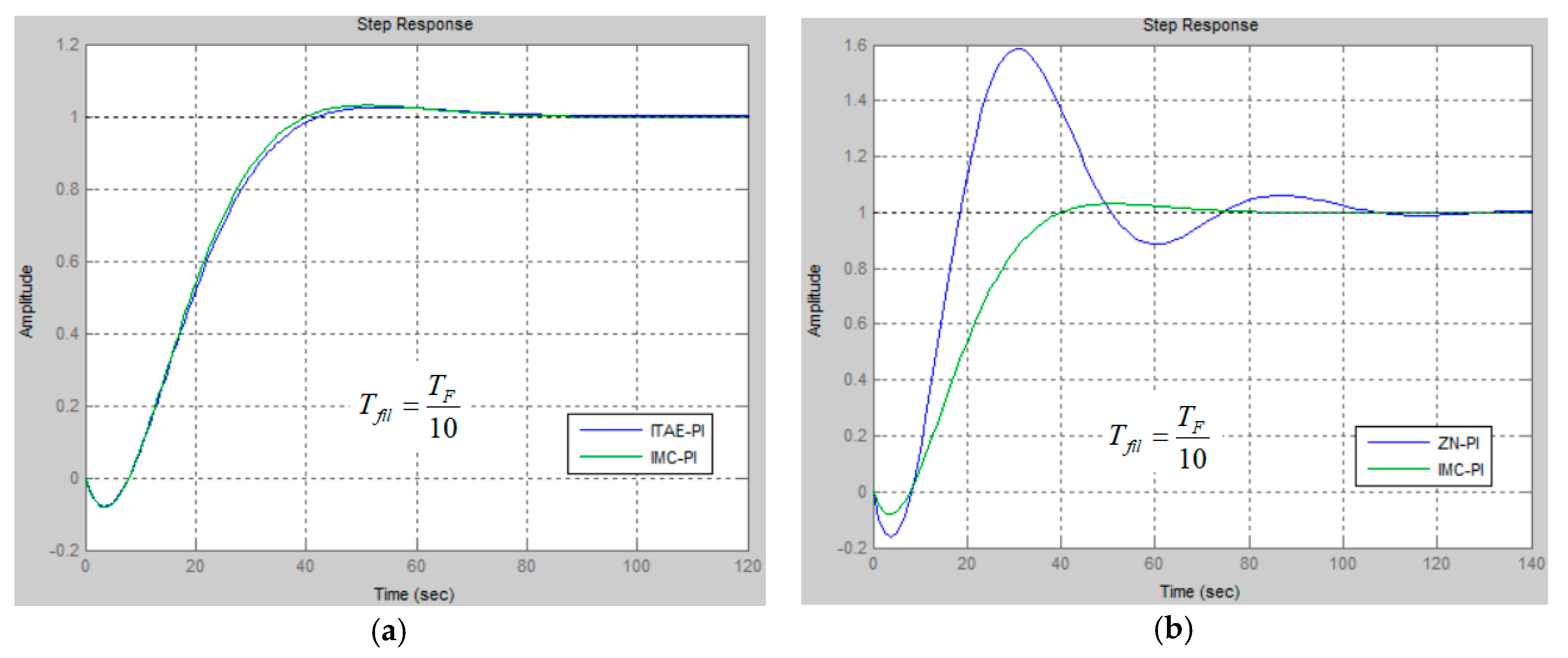
Using a PI controller (25) and the ITAE criterion for tuning the parameters (set-point tracking), where, according to [12]: ; , the indicial response in Figure 7a was obtained, presented in comparison to the indicial response obtained with IMC PI controller. According to Ziegler–Nichols criterion, the tuning parameters of the PI controller are [4]: ; .
6. Conclusions
The paper presents a mathematical model of the tank used in a chemical plant for obtaining the saturated steam from superheated steam and proposes different PID controllers, implemented for the temperature control.
Due to a very large overshoot, the use of the Ziegler–Nichols determined controller is not recommended. The controller designed by the ITAE criterion offers good performances, both in steady state and in transient regimes.
In the case of designing the IMC controllers described by (22) with approximation (18) for time delay and (25) with approximation (24) for time delay, the parameter influences the transient regime performances of the closed loop system. By varying the parameter , the time response can be changed relatively easily, adequately influencing the overshoot of the control system.
Conflicts of Interest
The author declare no conflict of interest.
References
- Smith, C.; Corripio, A. Principles and Practice of Automatic Process Control; John Wiley & Sons, Inc.: New York, NY, USA, 1997. [Google Scholar]
- Seborg, D.E.E.T.; Edgar, T.F.; Mellichamp, D.A. Process Dynamics and Control; John Wiley & Sons, Inc.: New York, NY, USA, 2011. [Google Scholar]
- Dulău, M. Sisteme de Conducere a Proceselor Continue; “Petru Maior” University of Târgu Mureș: Târgu Mureș, România, 2013. [Google Scholar]
- Lazăr, C.; Vrabie, D.; Carari, S. Sisteme Automate cu Regulatoare PID; MatrixRom: Bucharest, Romania, 2004. [Google Scholar]
- Khimani, D.; Mane, S.; Patil, M.D. Implementation of internal model control for flow control application. In Proceedings of the IEEE 9th International Conference on Industrial and Information Systems (ICIIS), Gwalior, India, 15–17 December 2014; pp. 1–6. [Google Scholar]
- Touati, N.; Saidi, I.; Soudani, D. Modified internal model control for unstable systems. In Proceedings of the IEEE International Conference on Advanced Systems and Electric Technologies (IC_ASET), Hammamet, Tunisia, 22–25 March 2018; pp. 352–356. [Google Scholar]
- Indirapriyadharshini, J.; Sivaranjani, T.; Gokila, R. Performance Analysis of Internal Model Control and Modified Internal Model Control for Two Tank Interacting and Non-Interacting Liquid System. Int. J. Innov. Technol. Explor. Eng. 2019, 8, 712–716. [Google Scholar]
- Dasgupta, S.; Sadhu, S.; Ghoshal, T.K. Internal Model Control based controller design for a Stirred Water Tank. In Proceedings of the IEEE India Conference (INDICON), Kolkata, India, 17–19 December 2010; pp. 1–4. [Google Scholar]
- Pathiran, A.; Jagadeesan, P. Design of internal model control dead-time compensation scheme for first order plus dead-time systems. Can. J. Chem. Eng. 2018, 96, 2553–2563. [Google Scholar] [CrossRef]
- Rivera, D.E.; Morari, M.; Skogestad, S. Internal Model Control. PID Controller Design. Process Des. Dev. 1986, 25, 252–265. [Google Scholar] [CrossRef]
- Garcia, C.; Morari, M. Internal model control. A unifying review and some new results. Ind. Eng. Chem. Process Des. Dev. 1982, 21, 308–323. [Google Scholar] [CrossRef]
- Rovira, A. Control Algorithm Tuning, and Adaptive Gain Tuning in Process Control. LSU Historical Dissertations and Theses. Ph.D. Thesis, Louisiana State University, Baton Rouge, LA, USA, 1981. [Google Scholar]
- Xue, D.; Chen, Y.; Atherton, D.P. Linear Feedback Control. Analysis and Design with MATLAB; SIAM: Philadelphia, PA, USA, 2007. [Google Scholar]
- Engineers Guide. Flow Diagram of Urea Production Process from Ammonia and Carbon-Dioxide. Available online: http://enggyd.blogspot.com/2010/09/flow-diagram-of-urea-production-process.html (accessed on 1 October 2020).
Figure 1.
The thermal system: (a) without delay; (b) with delay.

Figure 2.
The practical diagram implemented for the temperature control [14].
Figure 2.
The practical diagram implemented for the temperature control [14].

Figure 3.
The control block diagram.

Figure 4.
The conventional control block diagram.

Figure 5.
The internal model control (IMC) control block diagram.

Figure 6.
The indicial responses with IMC: (a) Proportional–Integral-Derivative (PID); (b) pressure indicator (PI).
Figure 6.
The indicial responses with IMC: (a) Proportional–Integral-Derivative (PID); (b) pressure indicator (PI).

Figure 7.
The indicial responses with PI controllers: (a) IMC and Integral of Time Multiplied by Absolute Error (ITAE); (b) IMC and Ziegler–Nichols.
Figure 7.
The indicial responses with PI controllers: (a) IMC and Integral of Time Multiplied by Absolute Error (ITAE); (b) IMC and Ziegler–Nichols.

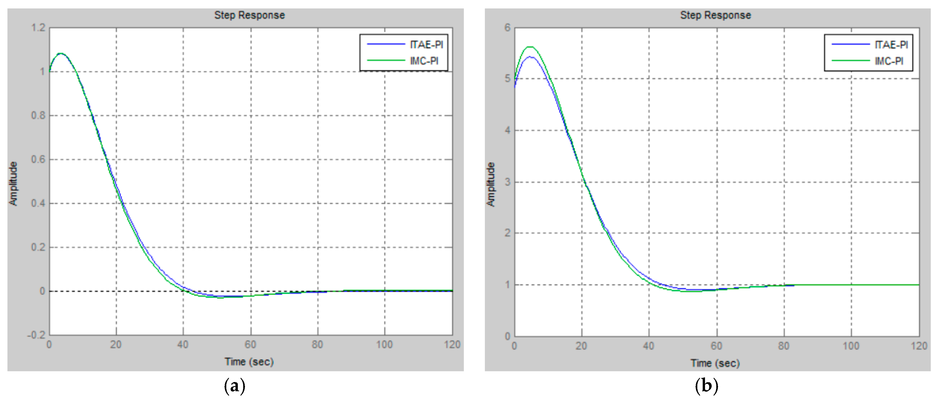
Figure 8.
The sensitivity functions: (a) ; (b) .

Publisher’s Note: MDPI stays neutral with regard to jurisdictional claims in published maps and institutional affiliations. |
© 2020 by the author. Licensee MDPI, Basel, Switzerland. This article is an open access article distributed under the terms and conditions of the Creative Commons Attribution (CC BY) license (https://creativecommons.org/licenses/by/4.0/).
Share and Cite
MDPI and ACS Style
Dulău, M. Control Strategies for Thermal Processes in Chemical Industry. Proceedings 2020, 63, 34. https://0-doi-org.brum.beds.ac.uk/10.3390/proceedings2020063034
AMA Style
Dulău M. Control Strategies for Thermal Processes in Chemical Industry. Proceedings. 2020; 63(1):34. https://0-doi-org.brum.beds.ac.uk/10.3390/proceedings2020063034
Chicago/Turabian StyleDulău, Mircea. 2020. "Control Strategies for Thermal Processes in Chemical Industry" Proceedings 63, no. 1: 34. https://0-doi-org.brum.beds.ac.uk/10.3390/proceedings2020063034