Generic Component-Based Mission-Centric Energy Model for Micro-Scale Unmanned Aerial Vehicles


1
Faculty of Computer Science, Otto-von-Guericke University, 39106 Magdeburg, Germany
2
AV-TEST GmbH, 39112 Magdeburg, Germany
*
Author to whom correspondence should be addressed.
†
These authors contributed equally to this work.
Drones 2020, 4(4), 63; https://0-doi-org.brum.beds.ac.uk/10.3390/drones4040063
Submission received: 31 July 2020
/
Revised: 14 September 2020
/
Accepted: 16 September 2020
/
Published: 25 September 2020
(This article belongs to the Special Issue Drone Mission Planning)
Abstract
:The trend towards the usage of battery-electric unmanned aerial vehicles needs new strategies in mission planning and in the design of the systems themselves. To create an optimal mission plan and take appropriate decisions during the mission, a reliable, accurate and adaptive energy model is of utmost importance. However, most existing approaches either use very generic models or ones that are especially tailored towards a specific UAV. We present a generic energy model that is based on decomposing a robotic system into multiple observable components. The generic model is applied to a swarm of quadcopters and evaluated in multiple flights with different manoeuvres. We additionally use the data from practical experiments to learn and generate a mission-agnostic energy model which can match the typical behaviour of our quadcopters such as hovering; movement in x, y and z directions; landing; communication; and illumination. The learned energy model concurs with the overall energy consumption with an accuracy over 95% compared to the training flights for the indoor use case. An extended model reduces the error to less than 1.4%. Consequently, the proposed model enables an estimation of the energy used in flight and on the ground, which can be easily incorporated in autonomous systems and enhance decision-making with reliable input. The used learning mechanism allows to deploy the approach with minimal effort to new platforms needing only some representative test missions, which was shown using additional outdoor validation flights with a different quadcopter of the same build and the originally trained models. This set-up increased the prediction error of our model to 4.46%.
1. Introduction
Unmanned Aerial Vehicles (UAVs) are used in more and more applications in the real world. These applications range from inspection tasks, e.g., bridges [1] and wind turbines [2], to agriculture applications like protection of deer from harvesters (https://www.theguardian.com/world/2014/apr/25/german-drones-protect-young-deer-combine-harvesters). However, most of these applications are still done using remotely piloted UAVs, even though the usage of autonomous quadcopters as replacements promises additional benefits like tighter surveillance and less cost. Consequently, the development of reliable, efficient and fully autonomous UAV systems is in the focus of current research [3,4,5,6]. Especially, swarms of UAVs promise high efficiency with low-cost UAVs. UAVs, in general, promise efficient deployment and manoeuvrability even in hardly accessible areas, for example, in natural disaster management [7]. The benefit in manoeuvrability comes at the cost of high energy consumption of the robots. Consequently, energy efficiency is a key concern in the development of quadcopter systems. Extending the mission time by using larger capacity batteries is limited because larger batteries can block the airflow below the rotors and add weight. To compensate blocked airflow and additional weight the quadcopter needs more power. Mission planning and energy-aware decision-making may provide an alternative to enhance the energy efficiency of a single quadcopter, but are limited because the degrees of freedom in designing and optimising a mission are limited. Swarm robotics may mitigate this problem through the inherent cooperation. A swarm of multiple robots has more energy resources than a single robot thus energy becomes scalable through the number of robots. Furthermore, intelligent cooperation enables more efficient resource usage. Additionally, scaling the swarm can minimise mission time and enhances robustness in case of failures. Examples of such swarm robotic behaviours are the works of Jatmiko et al. [8], Marchant and Tosunoglu [9] and Bayat et al. [10]. These algorithms focus on optimising mission time and scalability while solving a variety of different tasks [11,12]. However, the critical problem of energy efficiency is seldom investigated. Mostaghim et al. [13] designed an energy-efficient modification of the Particle Swarm Optimisation (PSO) Algorithm, which can be applied to quadcopter search missions. Bartashevich et al. [14] worked on energy-efficient quadcopter movement under environmental influences (especially wind). Mai et al. [15] proposed new metrics for optimisation algorithms, which take movement cost in the form of energy and time into account to evaluate existing optimisation algorithms regarding their applicability to swarm robotics. However, in all these works the energy model is very general, idealised and based on simple assumptions. Therefore, these energy models do not accurately represent the energy consumption of any real robot. This jeopardises the efficiency because the whole mission planning and run-time decision-making is based on the predictions of the energy model. Consequently, energy-efficient mission planning especially in the swarm use case mandate flexible and realistic energy models for swarm robotic platforms. This paper will provide a generic mission-agnostic energy model for UAVs, which is applied to an existing swarm robotic platform and tested regarding the achievable accuracy using real-world test flights.
2. State of the Art
Several authors in the field of swarm robotics develop behaviours that are energy efficient with respect to a specific energy model. These models are often idealised and do not accurately represent the energy consumption of a real robot. Mai et al. [15] use the travelled distance to approximate energy consumption of a robot. Mostaghim et al. [13] assume that energy is spent for certain manoeuvres like starting and landing and that mission time is a key factor for the energy consumption of quadcopters. Bartashevich et al. [14] only approximate the additional energy spend in the presence of external influences like wind and assume a fixed baseline consumption.
Dietrich et al. [16] present an energy model which is based on the analysis of empirical flight data only. The authors model the quadcopter as a fixed-weight object directly investing energy to move around in the air. The modelled flight behaviours are divided into three categories: Hovering, Horizontal Flight and Vertical Flight. In this model, the consumed energy of the quadcopter for hovering depends on the hover time only. The energy for horizontal and vertical movements is solely based on the flight angle and distance of the manoeuvre. The z-score of the validation flights showed results mostly lower than . This indicates strong similarity to the energy usage of the real copter. However, the energy model is very specific for the presented type of quadcopter. In consequence, the used methodology and the results cannot be transferred easily to other quadcopters.
The work of Di Franco and Buttazzo [17] presents an empirical energy model dependent on speed and acceleration of the quadcopter to be used for coverage path planning. The energy model was validated through autonomous flights of a quadcopter through a set of waypoints over a random area at a constant height. For this test mission, the real measured energy was compared to the estimated energy through the model resulting in a relative error of . The model is tightly coupled with the intended use case of the paper. The considered manoeuvres are limited to the ones created by the coverage path planning, which contains many angle turns. These movements are very specific movements for the used coverage path planning algorithm. The evaluation of the energy model is very limited, as only a single validation flight was conducted.
In the paper of Abdilla et al. [18] an endurance model for the ARDrone 2.0 is developed. The model combines a battery model of a Lithium-Polymer Battery (LiPo) battery and an energy consumption model for the quadcopter, based on momentum theory. In various test flights, the authors observed a similarity between the required power for manoeuvres and the power needed for hovering. Therefore, the authors only consider the hovering power in their final model. Two models of different complexity were tested. The most complete power model was tested by flying 27 different missions. The results showed a standard deviation of the estimated power of ~5% of the flight power. Tests with an identically constructed quadcopter resulted in model parameters which differed by 100%. Therefore, the authors considered this model to be sensitive to the specifics of the quadcopter used. A simpler model achieved a standard deviation of 10% and showed more robustness regarding the specifics of the used quadcopter.
A unique approach to reduce energy consumption is presented by Roberts et al. [19] and Dorigo et al. [3]. The authors show a mechanism to attach a quadcopter to the ceiling to disable the motors while still providing birds-eye view. Additionally, an endurance estimation model was developed for this set-up. Using the main assumption that the quadcopters thrust equals its weight while flying, the relationship between power consumption and thrust based on the used motor–propeller combination is characterised via static thrust measurements with a custom test rig. The resulting model combines the necessary power as the sum of the idle state power consumption and the power necessary to generate thrust equal to the total take-off weight. The model provides an endurance estimation with a maximum mean error of . Unfortunately, the paper uses a very restrictive movement model. However, the disambiguate between idle state and hovering consumption is very beneficial for swarm behaviour, because shutting down movement can be used by the decision-making to save energy (see Mostaghim et al. [13]).
Yacef et al. [20] developed a purely theoretical model based on equations for dynamic quadcopter movement, motor dynamics and battery dynamics. The aim of the model is the optimisation of energy consumption of a generic quadcopter. An approach towards validation was done through a simulation of vertical take-of missions with different trajectories and control inputs. The consumed energy for both missions was estimated and compared to the theoretically expected energy. Unfortunately, no real-world experiments and validation was done.
The discussed existing energy models show various drawbacks. Some are not mission-agnostic and therefore allow no prediction of individual movements. Others do not model individual components of the copter, which is unsuitable for swarm behaviour algorithms. The aim of our model, which is described in the next section, is to provide a generic energy model, which enables mission-agnostic precise energy prediction for swarm robotics platforms.
3. Model
In this section, we present the general concept of the energy model we created for the FINken3 quadcopter. This concept is generic and can also be applied to other robotic systems. Each quadcopter (or robot) is defined by a set of components. The energy usage of each component is defined by a specific set of parameters. The values of those parameters depend on the mission of the quadcopter. Finding and fitting the set of parameters to describe the energy consumption of a component is achieved by a grey-box approach. This approach combines expert knowledge about the copter to generate an energy model for each component and use regressions to tune the model parameters based on experimental data.
3.1. Components of a Quadcopter
A quadcopter is a complex technical system, which consists of multiple individual electrical and mechanical components. Typical components are Motors, Motor Drivers, Embedded Controllers, Batteries, Various Sensors, the Chassis and Cover Parts. Even though the electrical components are consuming energy from the battery, the mechanical parts influence the energy consumption just as much. Consequently, each quadcopter needs to be viewed as an appropriate collection of sub-assemblies.
Definition 1
(Quadcopter Q). A quadcopter Q is a collection of k components :
Definition 2
(Component ). A component of the quadcopter is a sub-assembly of the copter with a defined state and a power consumption at each point in time. The state of each component is defined by a vector of parameters observable at runtime .
The aim of our model is the estimation and prediction of energy drawn from the battery in a specific mission relevant situation. Therefore, we select components according to the observability of their energy consumption as well as the interaction between them. Preferable are components with easily observable parameters and minimal interaction with other sub-components. The state of a component is defined at each point in time by a set of observable parameters. Such parameters can either be a condition, characteristic or measurement. An example is the motor component (consisting of the four motor drivers, motors and propellers), whose energy consumption depends on the weight and acceleration of the copter.
The parameters of each component are defined through their parameter space , which each parameter is restricted to: . Each parameter of the quadcopter can influence multiple components at the same time. Consequently, the state of the copter can be described by the values of all parameters of a component, which are combined to a parameter vector of the global parameter space .
Definition 3
(Global Parameter Space ). The global parameter space is a Cartesian Product of all k parameter spaces of each component . The parameter vector is an element of the global parameter space
3.2. Description of Quadcopter Missions
The proposed energy model of Section 3.1 uses component specific parameters to infer the power consumption at each point in time.
Definition 4
(Mission). The mission is a total function which maps each time point t of the mission time frame to a parameter vector of the global parameter space. We assume this function to be deterministic, non-surjective and non-injective.
The mission function can be developed with the help of a set of help functions. Each helper function computes at least one parameter from the parameter space . The resulting mission function is the correctly ordered concatenation of the helper functions’ output.
To enable the energy model to be used in different missions, each mission needs to be translated to a time-series of parameter vectors to enable an energy consumption estimation at each point of time of the mission. A specific quadcopter mission defines the parameter vector of a quadcopter at each point in time during the mission time frame. This modelling is especially helpful if independent behaviour of the components of the copter needs to be modelled, like (de)activation of components. Typical mission helper function are step functions for components, which can be activated or deactivated or linear algebra equations in homogeneous 3D-coordinates to represent motion.
3.3. Power Function of Components
To compute the energy consumption of the quadcopter in a certain time frame of a mission, we assign each component of the quadcopter a power function , which maps the state of each component described by the parameter vector to an output power expressed as a real number. This power function uses the whole parameter vector of the quadcopter as input, even though it may only depend on individual parameters . The power function of the quadcopter is defined as the sum of power functions for all components. This reflects the law of conservation of energy:
To calculate the power of the quadcopter for a specific mission, the mission description function can be used to transform the mission time frame to the parameter vector space. Afterwards, the power function of the quadcopter can be used to transform the parameter vector at each point in mission time to a power.
Definition 5
(Energy Function). To estimate the energy needed for a manoeuvre in the time frame within the mission, we calculate the integral of the concatenated function, according to the physical relation of power and energy .
The power functions of the components contain the free parameters of this model. To parametrise the energy model for a quadcopter the power functions for each of its components must be modelled using an estimated power function and an error function :
A correctly modelled power function introduces a bounded error function , .
We consider three special types of power functions as generic templates for the components in a quadcopter: Constant Power Functions, Discrete Power Functions and Continuous Power Functions.
The most simplistic form of a power function of a component is the Constant Power Function. The characteristic of this function is that no has an influence on the drawn power. Consequently, the power of the component is not dependent on the state and therefore mission. The Constant Power Function is defined as
This type of power function can be applied to components which do not fluctuate in their power usage. Example for such components are static sensors and micro controllers with a constant power draw.
A second type of power function is the Discrete Power Function. This function enables a selection of the used power function based on the input parameter vector , according to
All need to define non-overlapping non-empty subsets of , where each represents a dedicated activation condition. This function type can be used to model components with discrete activation states like LEDs, additional motors or manipulators to interact with the environment.
The third type of power functions are Continuous Power Functions. We consider multivariate polynomials of degree o, which enable the representation of physical phenomena like inertia or drag with reasonable precision:
In general, not all parameters are necessary. Based on expert knowledge of the technical implementation of a component, a simplified polynomial may be used.
3.4. Machine Learning Approaches for Power Functions
A generic approach is to fit the energy model for a given quadcopter by first specifying the type of power function of each component and determine the coefficients through expert knowledge or experiments. Each type of power function has different coefficients that need to be estimated to adapt them to the component in question. To this end, three approaches are possible:
- White-Box
- This approach uses specific system knowledge to determine the necessary coefficients based on the physics of the system. Such approaches rely on either the electrical, dynamic or fluid system theory and the known behaviour of the component. Very few data are necessary for the approach, but it generally lacks in precision, because some effects are not modelled or some coefficients are hard to measure.
- Black-Box
- This approach views the component as a black box. The coefficients of the power functions of different components are fitted to the data using machine learning techniques like regressions, gradient descent or evolutionary algorithms. These aim to minimise in the learning process. The used models are typically neural networks or genetic programming. All these methods typically need a large amount of data from a sufficient set of environmental conditions to guarantee stable results. Additionally, hyperparameters need to be chosen manually by the user.
- Grey-Box
- This approach combines the first two approaches. It uses system knowledge to derive analytical power function with unknown coefficients from the behaviour of the component using expert knowledge. Afterwards, the coefficients are fitted to experimental data to parametrise the model. This approach needs far less experimental data than the black-box approach, but still enables adaptation to real hardware.
The benefit of the proposed generic model is the ability to select one of these approaches for each component individually. For sufficiently complex components like the motors of quadcopters we will aim for the Grey-Box approach, as it enables a precise model fitting to the hardware in question with reasonable effort to acquire training data.
3.5. An Energy Model for the FINken Quadcopters
To evaluate the generic energy model, we decided to use the FINken [4] quadcopters, which were developed in our lab. These copters are designed to be a modular research platform for indoor quadcopter and swarm robotics research. The main benefit of this platform in comparison to commercial ones is the option to easily adapt the sensory equipment. For these experiments we added an analogue current sensor to the internal power distribution of the copter to enable live current measurement. Another benefit is the option to log the measurement with high-speed to an on-board SD-Card, which enables fine-grained analysis of the behaviour of the copter.
Consequently, we implemented the presented energy model for the FINken3 [4] robot. To this end, we decomposed the quadcopter into several components. As the FINken3 (see Figure 1) is a modular quadcopter where each module can be plugged in, the decomposition was based on these modules. The modules where measured individually as far as possible. Some modules where combined to fit the component definition of the energy model (Definition 2).
The current draw of the motors cannot be measured directly. Consequently, we compute the power of the motors by measuring the overall power of the quadcopter and subtract the power draw of the other components. The decomposition of the FINken3 quadcopter showed the following individual components.
Motors are modelled through a Discrete Power Function transitioning between deactivated, idle and flying using five parameters: arming , height above ground and three axes accelerations . Three cases are distinguished: Off (not armed), Idle (armed and not flying) and Flying (armed and flying). The first two cases are modelled as Constant Power Functions with coefficients and . The third case as a Continuous Power Function in form of a multivariate polynomial of order three with the coefficient vector .
Motor Driver and Height Sensor are modelled through a Constant Power Function, because these sub-assemblies cannot be switched off:
Embedded Autopilot Board is modelled through a Constant Power Function, because the autopilot as the central unit of control cannot be switched off:
Sensor Interface Board with attached LEDs is modelled as a Discrete Power Function containing multiple Constant Power Functions, because the board itself cannot be switched off, but the eight attached LEDs draw current based on the selected colour and illumination. In the case of the FINken, only specific configurations are used for the LEDs. Four LEDs are used for camera tracking and have static colours, whereas 4 LEDs are used as an identification pattern:
Combining Equation (11) with a Constant Power Function for the tracking LEDs yields the final LED power function:
802.15.4 Transceiver is currently not using any power saving mechanisms, which enables us to model it using a Constant Power Function:
Remote Control Receiver is constantly receiving information from the remote control to be able to emergency shut off the copter and is modelled through a Constant Power Function:
GPS-Receiver draws constant power independent of GPS reception. It is modelled through a Constant Power Function:
It is important to model the last four components independently, because they can easily be attached and removed from each copter, which changes the copter’s energy consumption.
The Resulting Parameter Space is the Cartesian product of the parameter spaces of all components, because no two components use the same parameters: . With the corresponding parameters . The activation parameters for motors and the led configuration are directly defined in the mission and can be extracted from the mission program. The acceleration parameters can be acquired through various sources. The copter contains an on-board inertial measurement unit (IMU), which output turn rates and accelerations in all three axes. Another means of acquiring the values of the parameters is the usage of an external position tracking system and the computation of numerical derivatives.
In case of a fully equipped copter the final energy model is constructed from the power functions of the individual components, see Equations (8)–(15), through the application of Equation (2). The resulting model is
If components are removed from the copter, the energy model can easily be adapted because the respective parts of the energy model can be removed easily. A basic FINken3, for example, only consists of Motor, Motor Driver and Autopilot. The energy model for such a copter set-up is
The ability to adapt the energy model if components are attached or detached is very important for such a research platform, because the platform is frequently modified for different experiments. A second aspect of adaptability are the coefficients of the component energy models. These can be derived through measurement or in the case of the motor component it needs to be learned. Consequently, a modification of the copter, which incorporates large changes in weight or body shape needs an additional training phase for the motor energy model to adapt this model to the changes of the hardware.
4. Experiments
To parametrise the generic FINken quadcopter model developed in Section 3.5 data need to be generated through experimental flights, which are described and discussed in this section.
4.1. Experimental Set-Up
We conducted multiple experiments to parametrise and validate the model against the real-world behaviour of the copters. To estimate Constant Power Functions, we disassembled the quadcopter into the components and directly measured the power consumption of each component.
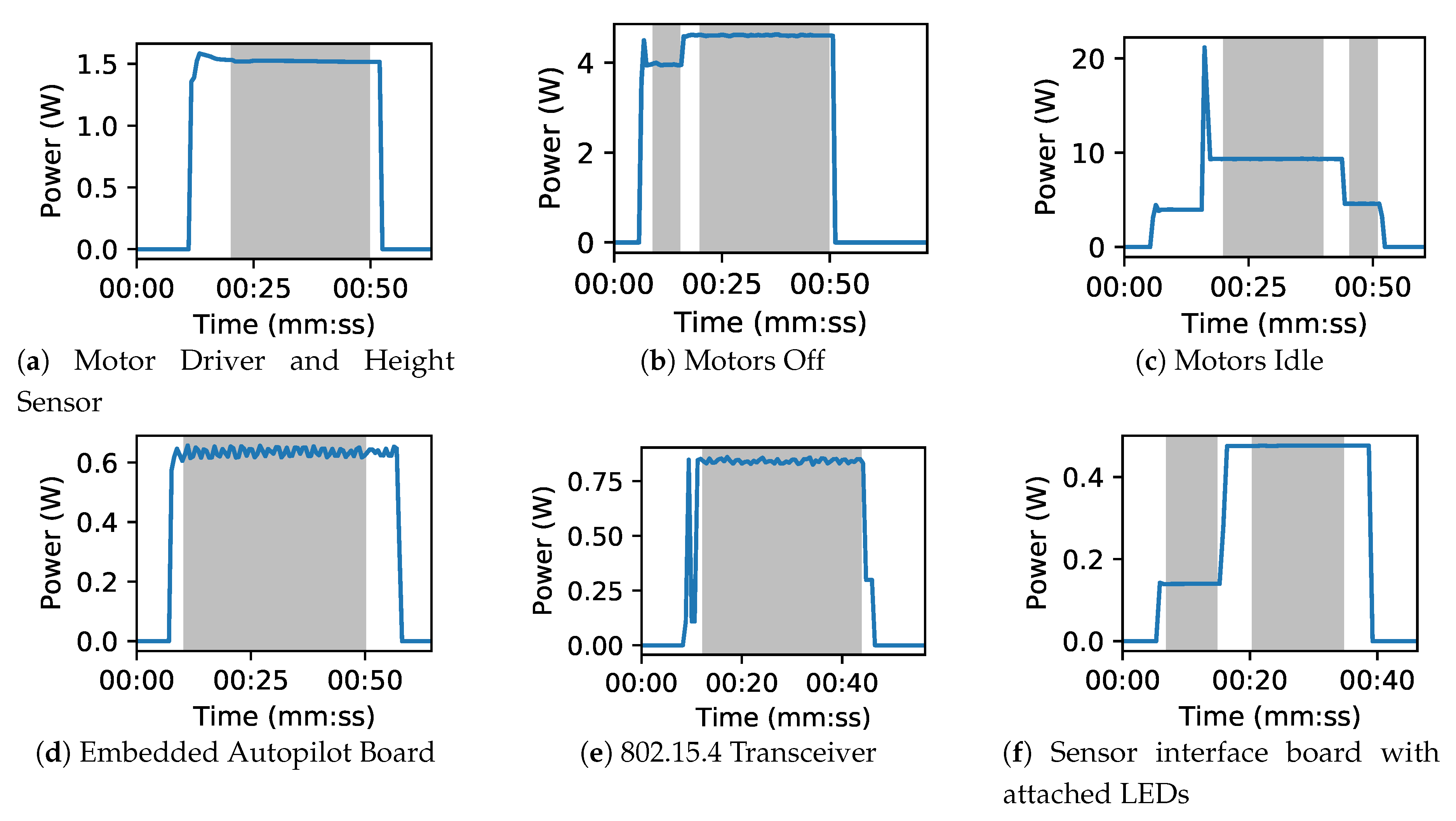
The measurements of the Constant Power Functions delivered the results shown in Figure 2. The power consumption in the relevant grey areas is clearly constant. Changes of power consumption exists for some components like the 802.15.4 Transceiver because of internal boot behaviour. Therefore, only the stable part of experimental data was used. The parameters were estimated using averaging on the whole selected sample subset. The resulting parameters are shown in Table 1.
The parameters of the Motor component need data gathered mid-flight using fully assembled quadcopters. To this end, we switched to the integrated current sensor of the FINken3 platform and logged the voltage, current and movement commands to an on-board SD-card. This allowed us to gather data with high speed. Internally, the FINken is capable of measuring the voltage of the Lithium-Polymer (LiPo) battery using the Analogue Digital Converter (ADC) of the micro-controller. The measurement has a precision of . The current is measured using an external Allegro ACS723LLCTR-40AB-T, which also uses the internal ADC of the autopilot. The current sensor needs to be calibrated, which limits its actual precision from the theoretical precision of . We considered multiple flight situations representing relevant areas of the parameter space. To enable position estimation of the quadcopter in the experiment, we use the on-board height sensor to estimate the z coordinate and a specialised tracking system installed in our lab, which is based on CNNs [21]. The precision of the tracking system is approximately cm. Additionally, we logged the gyroscope and acceleration data of the internal IMU, which is a MCU-6000 featuring g sensor range with a sensitivity of g for acceleration and s sensor range and a sensitivity of s. Through correlation analysis, we discovered that the acceleration data of the IMU provides better and faster data than the camera tracking system. Consequently, we used the internal IMU as data source for the acceleration parameters of the energy model. We conduct experimental flights hovering manually. Vertical movement was estimated using vertical flights changing height z within our laboratory (0.2 m–2.7 m). To estimate the horizontal movement, we conducted flights along the x and y coordinate (±2 m and ±1.5 m respectively) within our laboratory. These experiments provide us with the necessary data to estimate the coefficients of the third order multivariate polynomials using regression. We use different sets of training data to generate four differently trained models:
Hover Model (Hover) uses only the hovering movement without any movement in the or z coordinates as training data.
Vertical Model (Vert) uses in addition to the data used for the Hover Model data of movements in mainly z direction.
Horizontal Model (Horiz) uses in addition to the data used for the Hover Model data of movements mainly in direction.
Combined Model (Comb) uses all available movement data from the training flights.
These different training sets allow us to estimate the effect of the completeness of the training data towards the precision of the model. Additionally, it enables us to estimate the impact of the different types of movement regarding the overall energy consumption.
Additional test flights are conducted to serve as validation flights to compare measured energy on the copter with the results of our models, when applied to the mission specific parameters of the same flight. The mission specific flight parameters are taken from the internal sensors of the quadcopter, e.g., the IMU for flight behaviour. To test our model for overfitting we switched mid-flight between manual height control and autonomous height control, but kept manual horizontal control. Two validations flights were executed in our lab while three additional flight were executed outside with a different quadcopter of the same set-up. This enables us to estimate the sensitivity of the acquired model towards environmental conditions and platform specifics. The indoor flights followed the same pattern as the training flights. The outdoor flights were similar but scaled up in movement, because more space was available. The movement outdoors was along the edges of a square with a length of 30 m at a height of 3 m. The z movement was a linear movement between a height of 3 m and a height of 30 m. The horizontal movement speed was m/s, whereas the vertical movement speed was approx. m/s. All outdoor validation flights are done on the same day with low to no wind.
4.2. Results
Table 2 shows the results of the polynomial regression-based training of the power functions of the Motor component of the FINken 3 quadcopter. It is visible that all training flights are fitted homogeneously well. The cumulative relative error of each flight is less than 1%. Additionally, the standard deviation of the error for all flights is less than , which is very small considering the hover energy consumption of the copter (). Consequently, the used third-order polynomials are valid models for the energy consumption of the Motor component of a FINken copter.
Figure 3 shows the measured energy consumption and predicted energy consumption errors of the four different models, see Section 3.5 for the two indoor validation flights which were not included in the training data. The figures show that even for untrained flights, the models predict the consumed energy very accurately with an error of less than . The prediction error for the horizontal and the Combined Model are very similar. The Hover Model seems to be too simplistic and ignores the additional energy necessary for moving, as indicated by the generally lesser energy predicted by the Hover Model. However, for such a simplistic model the results are still fairly good indicating that the energy consumption of the FINken is strongly governed by the energy necessary for hovering. The Vertical Model shows a sudden jump in the middle of the flight for both validation flights. We assume that these jumps are caused by overfitting of the flights data in case of purely vertical flights. This may be induced because the vertical training flights do not include much horizontal movement. The horizontal flights contain vertical movements automatically, because the thrust needs to be adjusted when the quadcopter pitches or rolls. This induces vertical movement that is not perfectly compensated by the pilot or the autonomous height control of the copter creating data for the fitting of the vertical movement component.
The error statistics of the indoor validation flights, as shown in Table 3, shows the degradation of the Vertical Model for the validation flights. A relative error of more than 10% disqualifies the model for practical usage. The other three models are very close to an accumulated relative error of 1%. This shows that the models do estimate the consumed energy even for unknown flights very accurately.
Comparing the constant hover estimation with the extended movement model trained with horizontal flights shows an increase in estimation accuracy of approximately factor 3. This gain is bought by a more complex model and the need for more training flights to parametrise the model. It also shows the major domination of the energy consumption of a quadcopter by the energy necessary to hover. Consequently, an energy optimisation of swarms of quadcopters should aim to minimise flight time of the individual quadcopters. In the case of a landed copter the resulting energy consumption is still ~, which needs to be taken into account for long missions.
Table 4 show the results of the additional validation flights done with another copter of same build outdoors. Figure 4a shows the energy predictions of the same four models as used for the indoor flights. Interestingly, the sudden jump of the Vertical Model is gone. We suspect the height to be internally adapted by the used autopilot software. In the outdoor case, this was prevented by the used GPS receiver and/or the used barometer. Another explanation is the stronger variability of the flights because of environmental effects, which are not existent indoors. All models behave in a very similar manner for the outdoor flight and, similarly to the indoor flights, the Hover Model underestimates the used energy because it ignores movement. As visible in Figure 4c,d, for outdoor flights 2 and 3 the Hover Model behaved best, which may be an indication that the environment (wind) supported the movement and therefore reduced the energy needed for movement. This theory is supported by the performance of the Horizontal Model, which shows in all flights the largest error. Figure 4b–d show a generic trend of the models to converge to a static prediction error most of the time as visible in all flights for the Combined and Vertical Models. The Horizontal Model seems to be not as stable in the long run. This may be caused by the batteries providing different voltages over time, which necessitates an increase in throttle, which is not taken into account by the Horizontal Model. The performance of the Hover Model differs strongly between the individual flights, which indicates that the model is very sensitive to environmental conditions or the condition of the battery. However, it still shows on average good performance. The Combined Model, which was very good for the Indoor Validation Flights, showed a max. accumulated error of 6.316% with a max. deviation of power estimation of . Consequently, this model can be considered robust against slight environmental and minor platform changes, because the outdoor scenario was very favourable with nearly no wind and a very low flight height. For the short outdoor flights, the Hover Model performed even better with a deviation of and . This model performed reasonably well for the Indoor Validation Flights. Consequently, we can assume that the extended capabilities of modelling complex energy consumption of the Combined and Vertical Model create a stronger link to the platform specifics. The Hover Model, which uses less specifics of the platform, creates a more general prediction of the energy consumption of a copter. This is in line with the findings of Abdilla et al. [18].
In summary, the Hover Model is a good choice if a single model needs to be developed for swarms of quadcopters, whereas the Combined model is a good choice if accurate energy predictions are needed for individual copters.
5. Conclusions
In this paper, we showed a novel generic energy modelling approach for quadcopters. The approach provides predictions of the necessary energy for whole missions, but also arbitrary small parts of missions. The generic model was applied to the FINken3 quadcopters used in the SwarmLab. The process of applying the model to a specific hardware platform was shown, including the necessary experiments and the data analysis needed to infer the parameters of the model. We created four models using different amounts of training data using expert knowledge and fitted the models with training data from test flights. In the end, we verified these models against additional validation flights within and out of our laboratory to evaluate the accuracy of the predictions. The resulting accuracy of the best model showed an error of less than for the indoor validation on the same copter, which was used to train the model. This qualifies the model and the model-fitting process to be used to optimise missions of quadcopters both online and offline. Results using another copter in a different environment still showed an error less than if considering the best indoor model. The selection of the best overall model reduces the error to for the indoor validation flights and for the outdoor validation flights. The usage of another quadcopter for the outdoor flights also showed the generalisation achievable by the machine learning approach, which eases the generation of energy-models for fleets of similar quadcopters. The time the quadcopter spends flying turned out to be by far the most important factor in energy consumption. Our experiments show that the constant energy consumption of hovering predicts the energy consumption in the validation flights with less than error for short flights.
In the future, we aim to extend our model by a battery component model and a specific outdoor model to incorporate the effects of the environment like wind. Additionally, we want to extend the mission parameters of our implementation of the generic model to enable additional handling of heterogeneous swarms of quadcopters. Furthermore, we want to combine the model with energy-aware swarm behaviour algorithms to evaluate the resulting benefits. Finally, we aim to use the model in an evolutionary algorithm to optimise the set-up of our quadcopter platform as well as the usage of components of each quadcopter to minimise the global energy usage of fleets or swarms of quadcopters.
Author Contributions
Conceptualization C.S. and S.P.; methodology S.P.; software C.S., S.P., S.M. (Sebastian Mai); validation C.S. and S.M. (Sebastian Mai); formal analysis C.S. and S.P.; resources S.M. (Sanaz Mostaghim); data curation S.P.; writing–original draft preparation C.S., S.M. (Sebastian Mai), S.P.; writing–review and editing C.S. and S.M. (Sanaz Mostaghim); visualization S.P.; supervision S.M. (Sanaz Mostaghim); project administration S.M. (Sanaz Mostaghim); All authors have read and agreed to the published version of the manuscript.
Funding
This research received no external funding.
Conflicts of Interest
The authors declare no conflict of interest.
Abbreviations
The following abbreviations are used in this manuscript.
| CNN | Convolutional Neural Network |
| IMU | Inertial Measurement Unit |
| GPS | Global Positioning System |
| LED | Light Emitting Diode |
| SD-Card | Secure Digital Card |
| UAV | Unmanned Aerial Vehicle |
| PSO | Particle Swarm Optimisation |
| ADC | Analogue Digital Converter |
| LiPo | Lithium-Polymer Battery |
References
- Seo, J.; Duque, L.; Wacker, J. Drone-enabled bridge inspection methodology and application. Autom. Constr. 2018, 94, 112–126. [Google Scholar] [CrossRef]
- Shihavuddin, A.; Chen, X.; Fedorov, V.; Nymark Christensen, A.; Andre Brogaard Riis, N.; Branner, K.; Bjorholm Dahl, A.; Reinhold Paulsen, R. Wind turbine surface damage detection by deep learning aided drone inspection analysis. Energies 2019, 12, 676. [Google Scholar] [CrossRef] [Green Version]
- Dorigo, M.; Floreano, D.; Gambardella, L.M.; Mondada, F.; Nolfi, S.; Baaboura, T.; Birattari, M.; Bonani, M.; Brambilla, M.; Brutschy, A.; et al. Swarmanoid: A novel concept for the study of heterogeneous robotic swarms. IEEE Robot. Autom. Mag. 2013, 20, 60–71. [Google Scholar] [CrossRef] [Green Version]
- Steup, C.; Mai, S.; Mostaghim, S. Evaluation Platform for Micro Aerial Indoor Swarm Robotics; Technical Report FIN-003-2016; Otto-von-Guericke-Universität Magdeburg: Magdeburg, Germany, 2016. [Google Scholar]
- Zelazo, D.; Franchi, A.; Bülthoff, H.H.; Robuffo Giordano, P. Decentralized rigidity maintenance control with range measurements for multi-robot systems. Int. J. Robot. Res. 2015, 34, 105–128. [Google Scholar] [CrossRef] [Green Version]
- Stirling, T.; Roberts, J.; Zufferey, J.C.; Floreano, D. Indoor navigation with a swarm of flying robots. In Proceedings of the 2012 IEEE International Conference on Robotics and Automation, Saint Paul, MN, USA, 14–18 May 2012; pp. 4641–4647. [Google Scholar]
- Erdelj, M.; Król, M.; Natalizio, E. Wireless Sensor Networks and Multi-UAV systems for natural disaster management. Comput. Netw. 2017, 124, 72–86. [Google Scholar] [CrossRef]
- Jatmiko, W.; Jovan, F.; Dhiemas, R.; Sakti, A.M.; Ivan, F.M.; Fukuda, T.; Sekiyama, K. Robots implementation for odor source localization using PSO algorithm. WSEAS Trans. Circuits Syst. 2011, 10, 115–125. [Google Scholar]
- Marchant, W.; Tosunoglu, S. Rethinking Wildfire Suppression With Swarm Robotics. In Proceedings of the FCRAR 2016 29th Florida Conference on Recent Advances In Robotics, Miami, FL, USA, 12–13 May 2016; pp. 186–191. [Google Scholar]
- Bayat, B.; Crasta, N.; Crespi, A. Environmental Monitoring using Autonomous Vehicles: A Survey of Recent Searching Techniques. Curr. Opin. Biotechnol. 2017, 45, 76–84. [Google Scholar] [CrossRef] [PubMed] [Green Version]
- Bayındır, L. A review of swarm robotics tasks. Neurocomputing 2016, 172, 292–321. [Google Scholar] [CrossRef]
- Khaldi, B.; Cherif, F. An Overview of Swarm Robotics: Swarm Intelligence Applied to Multi-robotics. Int. J. Comput. Appl. 2015, 126, 31–37. [Google Scholar] [CrossRef]
- Mostaghim, S.; Steup, C.; Witt, F. Energy Aware Particle Swarm Optimization as Search Mechanism for Aerial Micro-robots. In Proceedings of the 2016 IEEE Symposium Series on Computational Intelligence (SSCI), Athens, Greece, 6–9 December 2016. [Google Scholar]
- Bartashevich, P.; Koerte, D.; Mostaghim, S. Energy-Saving Decision Making for Aerial Swarms: PSO-based Navigation in Vector Fields. In Proceedings of the 2017 IEEE Symposium Series on Computational Intelligence (SSCI), Honolulu, HI, USA, 27 November–1 December 2017; pp. 1848–1855. [Google Scholar]
- Mai, S.; Zille, H.; Steup, C.; Mostaghim, S. Multi-Objective Collective Search and Movement-based Metrics in Swarm Robotics. In Proceedings of the Genetic and Evolutionary Computation Conference Companion (GECCO), Prague, Czech Republic, 13–17 July 2019; pp. 387–388. [Google Scholar]
- Dietrich, T.; Krug, S.; Zimmermann, A. An Empirical Study on Generic Multicopter Energy Consumption Profiles. In Proceedings of the 2017 Annual IEEE International Systems Conference (SysCon), Montreal, QC, Canada, 24–27 April 2017; IEEE: Montreal, QC, Canada, 2017; pp. 406–411. [Google Scholar]
- Di Franco, C.; Buttazzo, G. Energy-aware coverage path planning of UAVs. In Proceedings of the 2015 IEEE International Conference on Autonomous Robot Systems and Competitions (ICARSC), Vila Real, Portugal, 8–10 April 2015; pp. 111–117. [Google Scholar]
- Abdilla, A.; Richards, A.; Burrow, S. Power and endurance modelling of battery-powered rotorcraft. IEEE Int. Conf. Intell. Robot. Syst. 2015, 2015, 675–680. [Google Scholar]
- Roberts, J.F.; Zufferey, J.C.; Floreano, D. Energy management for indoor hovering robots. In Proceedings of the 2008 IEEE/RSJ International Conference on Intelligent Robots and Systems, IROS, Nice, France, 22–26 September 2008; pp. 1242–1247. [Google Scholar]
- Yacef, F.; Rizoug, N.; Bouhali, O.; Hamerlain, M. Optimization of Energy Consumption for Quadrotor. In Proceedings of the 2017 Internation Micro Air Vehicle Conference and Flight Competition (IMAV), Madrid, Spain, 30 September–4 October 2017; IMAV: Toulouse, France, 2017; pp. 215–222. [Google Scholar]
- Hoyer, L.; Steup, C.; Mostaghim, S. A Robot Localization Framework Using CNNs for Object Detection and Pose Estimation. In Proceedings of the IEEE Symposium Series on Computational Intelligence (SSCI), Bangalore, India, 18–21 November 2018; IEEE: Bangalore, India, 2018; pp. 1388–1395. [Google Scholar]
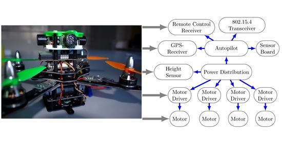
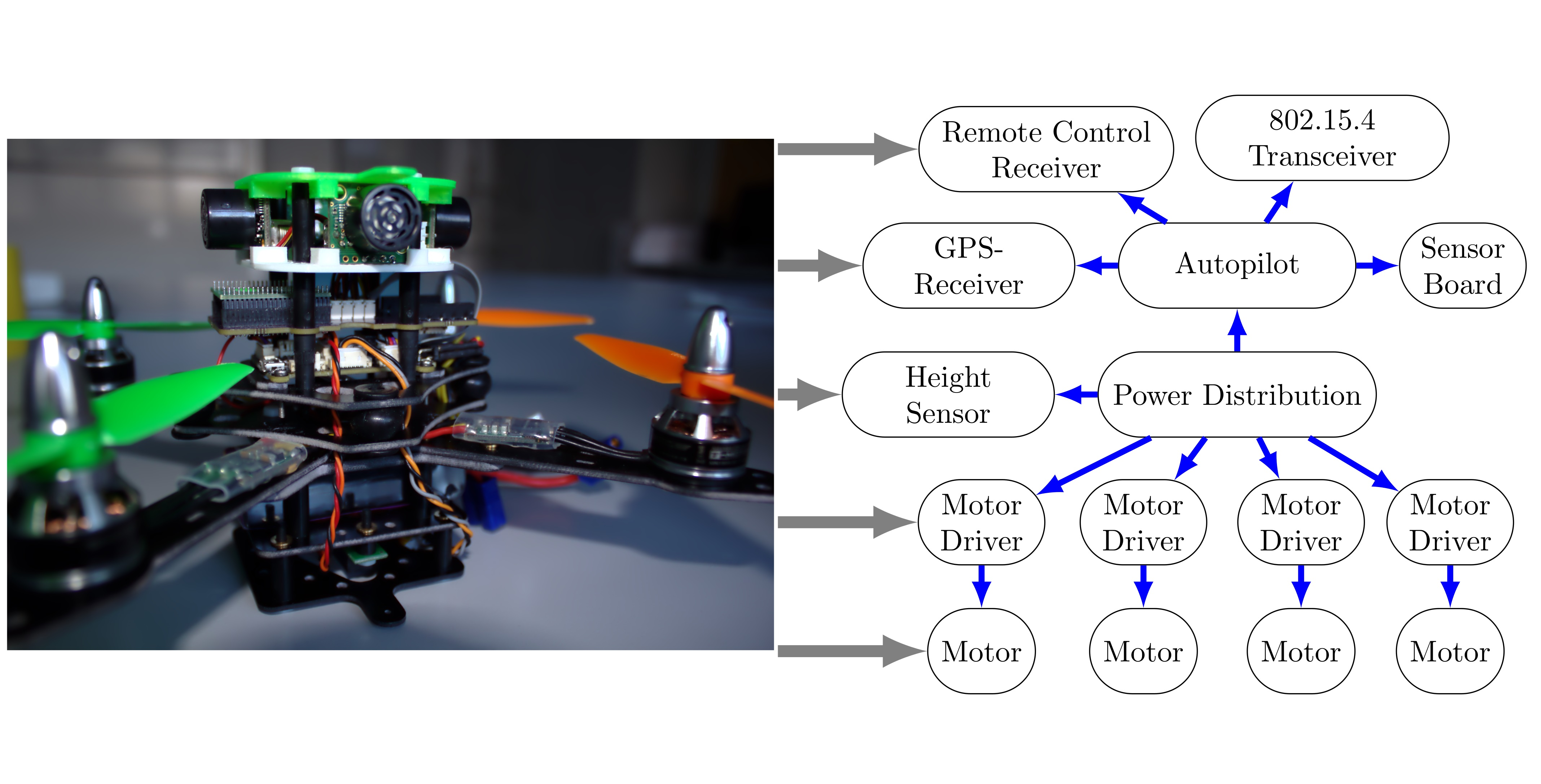
Figure 1.
Illustrations of the FINken Swarm of Quadcopters Platform. The left figure (a) shows a closeup picture of an example FINken3 quadcopter. The right figure (b) shows a schematic of the connections of components within the quadcopter.
Figure 1.
Illustrations of the FINken Swarm of Quadcopters Platform. The left figure (a) shows a closeup picture of an example FINken3 quadcopter. The right figure (b) shows a schematic of the connections of components within the quadcopter.

Figure 2.
Results of the static power measurements of the Components. The grey area indicates the used samples to derive the parameters. Multiple grey areas indicate different areas used for different Constant Power Functions within a Discrete Power Function.
Figure 2.
Results of the static power measurements of the Components. The grey area indicates the used samples to derive the parameters. Multiple grey areas indicate different areas used for different Constant Power Functions within a Discrete Power Function.

Figure 3.
Estimation results and error of differently trained models tested in two indoor validation flights. The two figures on the top (a,b) show the measured and predicted energy values for the two indoor validation flights. The two bottom figures (c,d) show the prediction error of the two indoor validation flights.

Figure 4.
Estimation results and errors of differently trained models tested in three outdoor validation flights. The top left figure (a) shows the measured and predicted energy values of the used quadcopter for the first outdoor validation flight. The top right (b), bottom left (c) and bottom right (d) figures show the error of the prediction for the three outdoor validation flights.


Table 1.
Results of the measurement of the Constant Power Function parameters of the energy model of the FINken. The first column indicates the part of Figure 2, which shows the measurement results.
Table 1.
Results of the measurement of the Constant Power Function parameters of the energy model of the FINken. The first column indicates the part of Figure 2, which shows the measurement results.
| Figure | Parameter | Value in W | Standard Deviation |
|---|---|---|---|
| Figure 2a | 1.52 | 0.0037 | |
| Figure 2b | 4.60 | 0.0082 | |
| Figure 2c | 9.33 | 0.0113 | |
| Figure 2d | 0.63 | 0.0135 | |
| Figure 2e | 0.84 | 0.0095 | |
| Figure 2f | 0.13 | 0.0001 | |
| Figure 2f | 0.47 | 0.0003 |
Table 2.
Results of the regression fitting of all experimental flights.
| Training | Flight 1 Comb | Flight 2 Comb | Flight 3 Comb | Flight 1 Hover | Flight 2 Hover | Flight 1 Horiz | Flight 2 Horiz | Flight 1 Vertical |
|---|---|---|---|---|---|---|---|---|
| mean | 0.0462 | 0.0345 | 0.0851 | 0.0095 | 0.0177 | 0.0273 | 0.0705 | 0.0270 |
| std | 0.0322 | 0.0180 | 0.0279 | 0.0055 | 0.0043 | 0.0186 | 0.0176 | 0.0152 |
| 25%-quantile | 0.0153 | 0.0197 | 0.0721 | 0.0044 | 0.0153 | 0.0119 | 0.0656 | 0.0139 |
| 50%-quantile | 0.0410 | 0.0351 | 0.0992 | 0.0093 | 0.0173 | 0.0222 | 0.0758 | 0.0309 |
| 75%-quantile | 0.0759 | 0.0529 | 0.1038 | 0.0146 | 0.0211 | 0.0434 | 0.0810 | 0.0410 |
| max | 0.1018 | 0.0607 | 0.1106 | 0.0199 | 0.0263 | 0.0640 | 0.0902 | 0.0478 |
| 1.5313 | 0.1860 | 1.9742 | 0.0719 | 0.8129 | 0.8801 | 0.8100 | 0.0008 |
Table 3.
Performance results of the four generated energy estimation models applied to the two indoor validation flights. Dark green fields highlight best results. Light green fields highlight second best results.
Table 3.
Performance results of the four generated energy estimation models applied to the two indoor validation flights. Dark green fields highlight best results. Light green fields highlight second best results.
| Validation | Flight 1 | Flight 2 | ||||||
|---|---|---|---|---|---|---|---|---|
| Model | Hover | Vert | Horiz | Comb | Hover | Vert | Horiz | Comb |
| mean | 0.0866 | 0.2231 | 0.0280 | 0.0362 | 0.0218 | 0.1087 | 0.0367 | 0.0186 |
| std | 0.0728 | 0.2311 | 0.0164 | 0.0277 | 0.0121 | 0.1188 | 0.0104 | 0.0076 |
| 25%-quantile | 0.0128 | 0.0126 | 0.0151 | 0.0181 | 0.0121 | 0.0132 | 0.0341 | 0.0124 |
| 50%-quantile | 0.0699 | 0.0675 | 0.0286 | 0.0253 | 0.0220 | 0.0305 | 0.0391 | 0.0199 |
| 75%-quantile | 0.1487 | 0.4287 | 0.0377 | 0.0542 | 0.0322 | 0.2346 | 0.0437 | 0.0249 |
| max | 0.2284 | 0.6310 | 0.0686 | 0.1046 | 0.0448 | 0.3544 | 0.0502 | 0.0315 |
| 4.4622 | 12.4032 | 1.3300 | 2.0428 | 0.9950 | 10.3208 | 1.3155 | 0.4166 | |
Table 4.
Performance results of three of the four generated energy estimation models applied to the three outdoor validation flights. The Horizontal Model did not produce good results and is omitted for clarity. Dark green fields highlight best results. Light green fields highlight second best results.
| Validation | Flight 1 | Flight 2 | Flight 3 | ||||||
|---|---|---|---|---|---|---|---|---|---|
| Model | Hover | Vert | Comb | Hover | Vert | Comb | Hover | Vert | Comb |
| mean | 0.0456 | 0.0116 | 0.0317 | 0.0597 | 0.1127 | 0.1024 | 0.0555 | 0.0964 | 0.1373 |
| std | 0.0294 | 0.0077 | 0.0218 | 0.0197 | 0.0353 | 0.0313 | 0.0281 | 0.0509 | 0.0712 |
| max | 0.1306 | 0.0293 | 0.0648 | 0.0833 | 0.1670 | 0.1504 | 0.1094 | 0.1588 | 0.2340 |
| 2.7085 | 0.3777 | 1.2639 | 0.1630 | 3.1661 | 3.2976 | 2.1741 | 4.1327 | 6.3156 | |
© 2020 by the authors. Licensee MDPI, Basel, Switzerland. This article is an open access article distributed under the terms and conditions of the Creative Commons Attribution (CC BY) license (http://creativecommons.org/licenses/by/4.0/).
Share and Cite
MDPI and ACS Style
Steup, C.; Parlow, S.; Mai, S.; Mostaghim, S. Generic Component-Based Mission-Centric Energy Model for Micro-Scale Unmanned Aerial Vehicles. Drones 2020, 4, 63. https://0-doi-org.brum.beds.ac.uk/10.3390/drones4040063
AMA Style
Steup C, Parlow S, Mai S, Mostaghim S. Generic Component-Based Mission-Centric Energy Model for Micro-Scale Unmanned Aerial Vehicles. Drones. 2020; 4(4):63. https://0-doi-org.brum.beds.ac.uk/10.3390/drones4040063
Chicago/Turabian StyleSteup, Christoph, Simon Parlow, Sebastian Mai, and Sanaz Mostaghim. 2020. "Generic Component-Based Mission-Centric Energy Model for Micro-Scale Unmanned Aerial Vehicles" Drones 4, no. 4: 63. https://0-doi-org.brum.beds.ac.uk/10.3390/drones4040063