Development, Modeling and Control of a Dual Tilt-Wing UAV in Vertical Flight


1
Laboratoire Franco-Mexicain d’ Informatique et Automatique, UMI LAFMIA 3175 CNRS-CINVESTAV, Av. IPN 2508, San Pedro Zacatenco, Ciudad de México 07360, Mexico
2
Heudiasyc, Université de Technologie de Compiègne, CNRS, CS 60 319, 60 203 Compiègne, France
3
Instituto Politécnico Nacional, Escuela Superior de Ingeniería Mecánica y Eléctrica UP Ticomán, Av. Ticomán 600, San José Ticomán, Ciudad de México 07340, Mexico
*
Author to whom correspondence should be addressed.
Drones 2020, 4(4), 71; https://0-doi-org.brum.beds.ac.uk/10.3390/drones4040071
Submission received: 14 October 2020
/
Revised: 14 November 2020
/
Accepted: 15 November 2020
/
Published: 25 November 2020
Abstract
:Hybrid Unmanned Aerial Vehicles (H-UAVs) are currently a very interesting field of research in the modern scientific community due to their ability to perform Vertical Take-Off and Landing (VTOL) and Conventional Take-Off and Landing (CTOL). This paper focuses on the Dual Tilt-wing UAV, a vehicle capable of performing both flight modes (VTOL and CTOL). The UAV complete dynamic model is obtained using the Newton–Euler formulation, which includes aerodynamic effects, as the drag and lift forces of the wings, which are a function of airstream generated by the rotors, the cruise speed, tilt-wing angle and angle of attack. The airstream velocity generated by the rotors is studied in a test bench. The projected area on the UAV wing that is affected by the airstream generated by the rotors is specified and 3D aerodynamic analysis is performed for this region. In addition, aerodynamic coefficients of the UAV in VTOL mode are calculated by using Computational Fluid Dynamics method (CFD) and are embedded into the nonlinear dynamic model. To validate the complete dynamic model, PD controllers are adopted for altitude and attitude control of the vehicle in VTOL mode, the controllers are simulated and implemented in the vehicle for indoor and outdoor flight experiments.
1. Introduction
In recent times, many UAV types have been developed with the purpose of expanding their features, flight modes, applications, missions, etc. Actually, UAVs can be classified into three groups: fixed-wing UAVs (airplane), rotary-wing UAVs (Multi-rotor) and hybrid UAVs.
A hybrid UAV combines the capabilities of a fixed-wing (large cruising speed) and a rotary-wing (vertical take-off and landing) by means of their three flight modes: VTOL, transition and CTOL. Based on whether or not the fuselage tilts, hybrid UAV can be further divided into two categories: convertiplane and tailsitter.
Tailsitter type vehicles perform the transition maneuver without requiring additional actuators, which reduces the weight, and are mechanically simpler. However, they have the following disadvantages: (1) they need a stronger tail to withstand the weight of the vehicle and the impacts during takeoff and landing; (2) while the tail is in contact with the ground, the ailerons do not generate pitch and roll torques; (3) when they are operated by remote pilots, they require expert pilots; (4) during hovering, this configuration has greater drag because the area exposed to crosswinds include the wing and fuselage.
On the other hand, tilt-rotor and tilt-wing are some examples of convertiplanes, both vehicles can perform the transition between VTOL and CTOL flight modes by means of a tilt mechanism that changes the angle of the rotors or the wings with rotors. In the case of tilt-rotor aircraft, the motors are fixed at the tip of the wings. Therefore, the wings are required to be shorter and, consequently, have less lift. Also, if the wing and rotors tilt together, like tilt-wing UAV, the airflow produced by the rotors will not be reduced by the interference with the wings, unlike the tilt-rotor case.
Due to a change of angle of the wings and rotors, tilt-wing UAVs present the following aerodynamic advantages: (1) minimum drag and down wash on the wings, since the wings are always aligned with the rotor; (2) in transition flight mode, the wings will start generating lift and drag because there will be an increase in speed at the same time, and even though the lift to drag ratio is low under the transition phase, the tilt-wing will still generate a fair amount of lift, meaning that the UAV will be able to utilize smaller rotors and become more efficient in terms electric current consumption as long as it can overcome the drag [1].
In the area of tilt-rotors, there has been more progress and focus in the last years. In reference [2,3,4] are presented vehicles with four, three and two rotors in addition to the main rotor, that have been a source of research for their different flight modes, from the control design to experimental flight tests. However, the area of the tilt-wings has been a growing area of research and development. Vehicles as SUAVI [5], JAXA’s “AKITSU” QTWUAV [6] and QTW QUX-02 [7] are some of the quad tilt-wing UAVs having four rotors located on the leading edges of the four identical wings at the front and rear of vehicle. The wing–rotor pairs can be tilted from vertical to horizontal position for the transition between flight modes.
Unlike tilt-rotor UAVs, the study focusing on the tilt-wing UAV is mostly the quad tilt-wing vehicle, due to its structural design similar to quadrotor. In reference [8] the authors present Tri tilt-wing UAVs where the thrust is generated by two main rotors and a tail rotor that stabilizes pitch, however, the paper focuses only on hover flight. On the other hand, the German DHL company [9], developed a dual tilt-wing UAV, where the thrust is generated only by two main rotors, nevertheless, there is no evidence of the vehicle development (structural design, control design, simulations, experimental tests, etc.).
Since the thrust is generated by two rotors, the Dual tilt-wing UAV presents a great stability challenge in its three flight modes. However, the electric current consumption decreases, the vehicle’s weight is smaller than the Tri or Quad tilt-wing, so the flight time increases.
In investigations based on the study of tilt-wing UAVs, complete dynamic models have been developed that include wing’s aerodynamic characterization or the study of the propeller effects. However, the study is only proposed in the horizontal flight mode or specific flight conditions. In reference [10], Benkhoud and Bouallegue considered the wing’s lift and drag forces only for horizontal and transition flight modes, as function of linear velocity ( and ), tilt () and attack () angles. Their motion equations for VTOL flight mode are similar to those of a Quadrotor. Additionally, in reference [11], Masuda and Uchiyama considered uncertainties such as wind in the model, and the aerodynamic coefficients were obtained by wind tunnel experiments. In reference [12], Cetinsoy et al. in addition to wind tunnel experiments, they performed ANSYS simulations to obtain the wing’s aerodynamic coefficients. They consider that the total thrust and the desired attitude angles are functions of the wing angles, this effect is not studied for quadrotors. In reference [13], Garcia et al. besides the angle of attack, they include the sideslip angle in the mathematical model. They also accounted for the propeller effect (Propeller Momentum Theory) to obtain the aerodynamic behavior of the vehicle in horizontal flight. Other papers as [8,14] mention that mounting the tilt-wings does not affect a fundamental operation of the Quadrotor, likewise, the additional aerodynamic forces exerted on the body and the forces produced by the flow of air from the propellers over the wing profile are neglected.
The present paper deals with a Dual tilt-wing which, to the best of our knowledge, has not yet been treated in the literature. For VTOL flight mode, the vehicle has two main rotors that are located on the leading edges of the two wings and two ailerons that are located on the trailing edges of the wings as control surfaces. For the transition flight mode, the wings together with the rotors are tilted from 90 to 0 degrees. The wings can either tilt together or independently. Furthermore, each wing has a control surface or aileron that can be used for controlling the pitch and yaw angles. Finally, for horizontal flight mode it is similar to a fixed-wing, with two rotors, two ailerons, an elevator and a rudder on the empennage as control surfaces.
The main contribution of this paper is to provide the UAV’s complete dynamical model, namely, for its different flight modes (vertical flight, transition and horizontal flight), because many dynamic models of tilt-wing UAVs are 3, 4 or more rotors and one or two fixed-wings [10,11,12]. The stabilization of those vehicles can be achieved more easily since they have more actuators to generate the necessary torques to stabilize the attitude of the aircraft. Furthermore, the mathematical models presented are just a combination of the models of a multi-rotor and a fixed wing and the aerodynamic studies are not presented in depth, therefore, are different to the model we study.
The non-linear dynamic model is obtained using the Newton–Euler formulation, the model includes aerodynamic effects, as the drag and lift forces of the wings which are a function of: (1) the airstream generated by the rotors; (2) the cruise speed; (3) the tilt angle which also can be used to control yaw and angle of attack.
The airstream velocity generated by the rotors is studied in a test bench. Later, the projected area on the UAV wing that is affected by the airstream generated by the rotors is specified and 3D aerodynamic analysis is performed for this region.
Aerodynamic coefficients of the UAV in VTOL mode caused by the wing, empennage and fuselage are calculated by using Computational Fluid Dynamics method (CDF) and are embedded into the nonlinear dynamic model.
Although the mathematical model presented includes all flight conditions of tilt-wing UAV, i.e., hover flight, transition and horizontal flight. In this paper, we focus only on simulation, the control algorithm and vertical mode flight tests. Therefore, to validate the dynamic model, PD controllers are adopted for altitude and attitude control for stabilizing the hover flight mode which is a critical phase of operation since normally airplanes do not perform hover flights. The controllers are simulated and implemented in the vehicle for real-time flight experiments.
The rest of the paper is organized as follows: Section 2 contains the Dual tilt-wing UAV complete dynamic model. In Section 3, modeling parameters are obtained. In Section 4, the dynamic model and the PD controllers are simulated and implemented for altitude and attitude control of the UAV in VTOL mode. The simulation results are analyzed. Subsequently, the real-time flight experiments results of UAV in VTOL mode are presented. Finally, Section 5 concludes the paper and future work is presented.
2. Methods
In this section, the UAV complete dynamic model is presented, aerodynamic effects are considered for its different flight modes. The model is obtained by employing the Euler-Newton formulation for each of its 6-degrees-of-freedom (6-DOF).
2.1. Equations of Motion
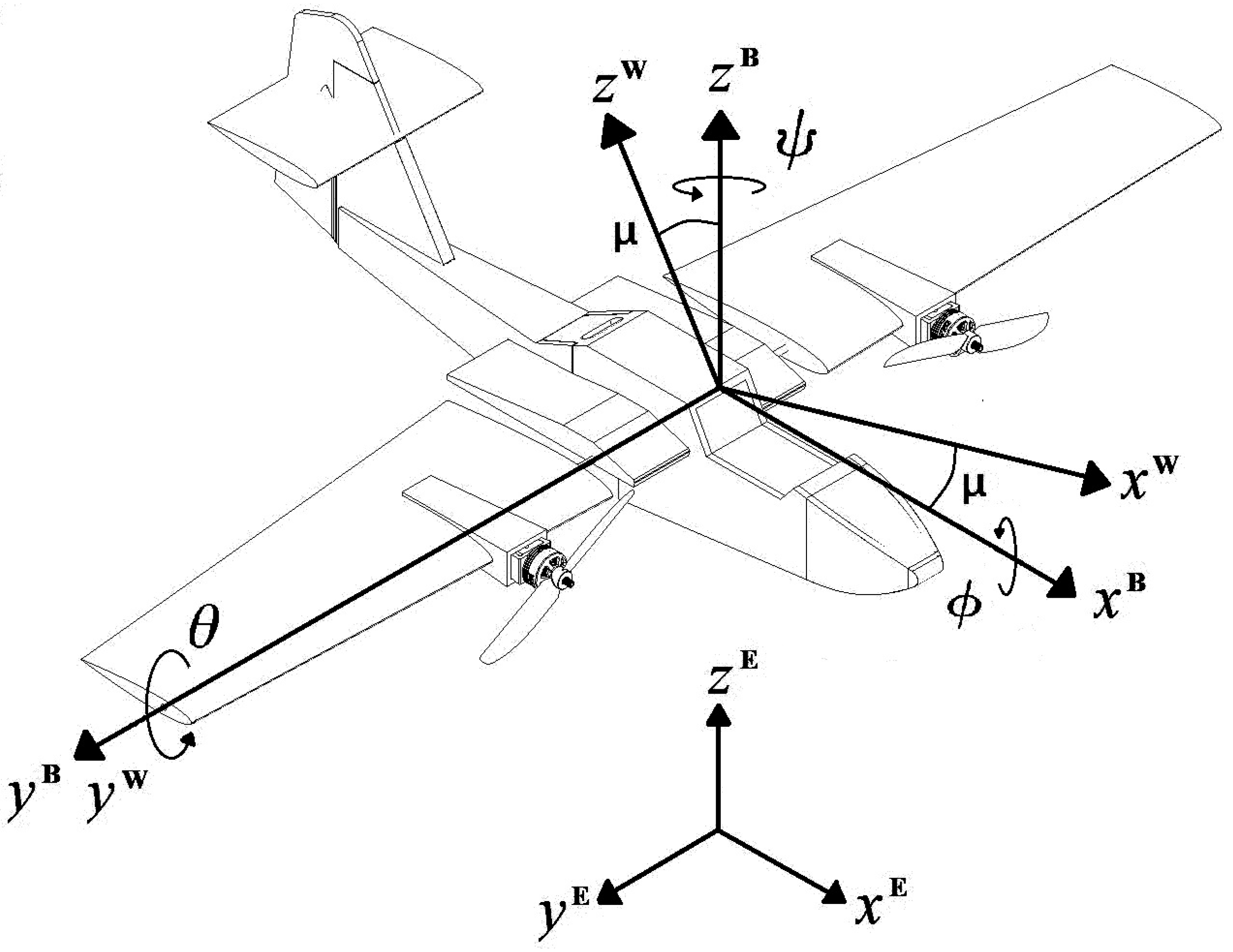
Consider each element as a rigid-body in the inertial reference system, with the gravity center (cg) coincident with the aerodynamic center (ca). denotes the earth fixed inertial reference frame, denotes the body fixed reference frame with origin in the cg, denotes the mobile aerodynamic referential with origin in the ca (Figure 1).
Assuming the generalized coordinates as , where denotes the vehicle position relative at the inertial frame and are the three Euler angles, roll, pitch and yaw respectively and represent the UAV attitude.
For transforming the axes from the body frame to the inertial frame, the rotation matrix is defined, where and .
For transforming the axes from the mobile aerodynamic referential to body frame, the rotation matrix is defined, where is the tilt angle of the tilt mechanism of wing and rotor [15,16].
Therefore, the UAV complete dynamic model is obtained, where the translational motion is based on Newton’s second law with respect to inertial reference frame and the rotational motion with Euler’s law with respect to body fixed reference frame [17].
where and are the forces and moments acting on the vehicle, is the UAV mass, denotes the linear acceleration, describes the angular velocity and the angular acceleration according to the Euler angles, with , and the rotation matrix R defined as:
Furthermore, describes the inertia tensor matrix, whose value depends on the body mass distribution, if the body symmetry on the plane is considered and the remaining inertia products are low compared to the main moments, the inertia tensor is approximated by:
2.1.1. Translational Dynamic
The total forces () acting on the vehicle is the sum of the rotors forces () and the aerodynamic loads (), .
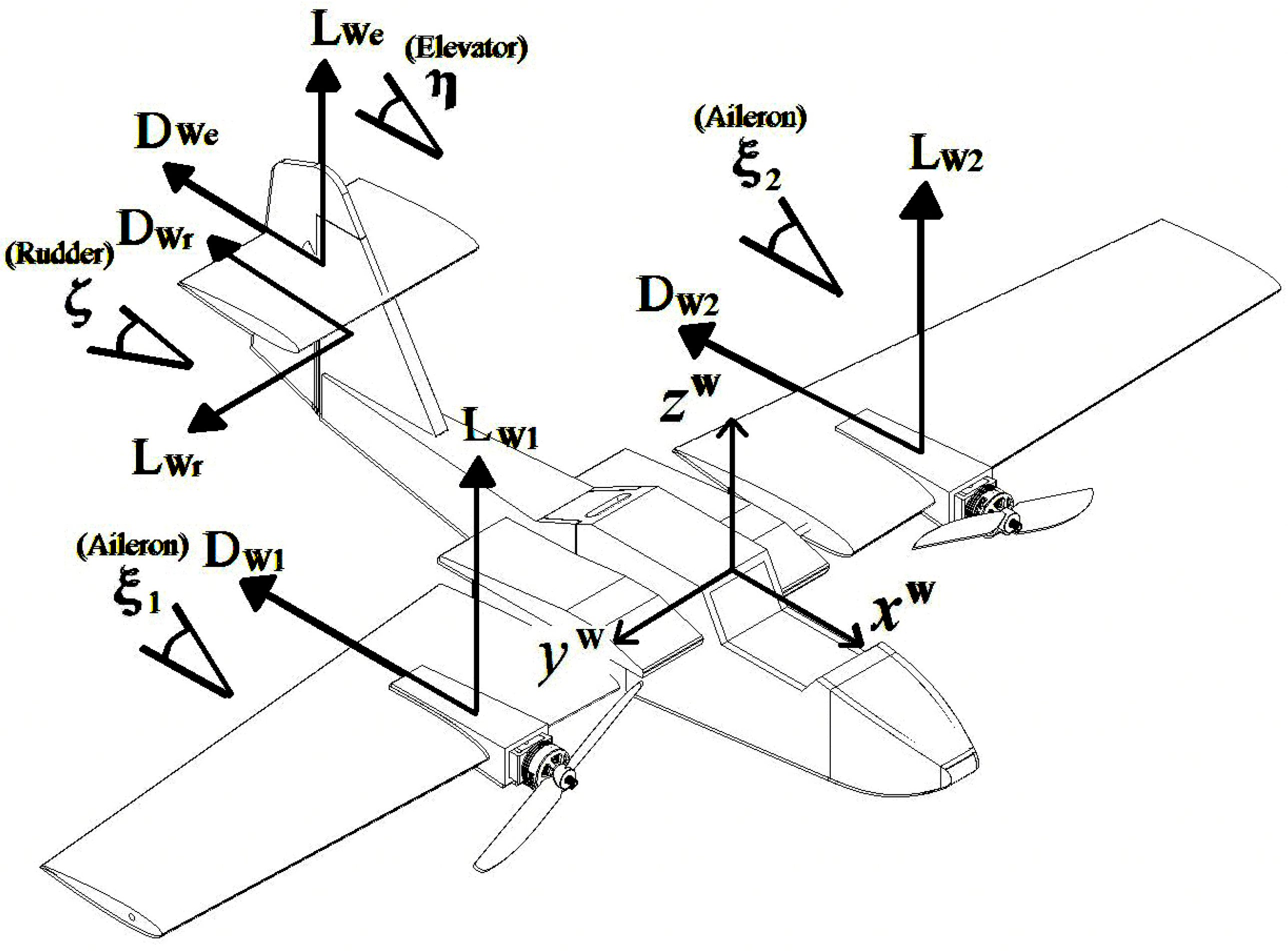
The vehicle consists of two rotors generating the thrust force for the vertical flight mode and a thrust force for the horizontal flight mode. With a fuselage and an empennage that include their aerodynamic effect in conjunction with two wings that generate aerodynamic forces as a function of the angle of attack, the control surfaces (ailerons, elevator and rudder), relative wind velocity and airstream generated by the rotors.
where L is the aerodynamic lift and D is the aerodynamic drag of the wings (W), the horizontal stabilizer (We) and the vertical stabilizer (Wr), (Figure 2).
2.1.2. Rotational Dynamic
The total moments () acting on the vehicle is the sum of the main moments provided by the control surfaces (), the gyroscopic moment generated by the variation of the propeller rotation axis (), and the drag moment () due to the propeller drag force, .
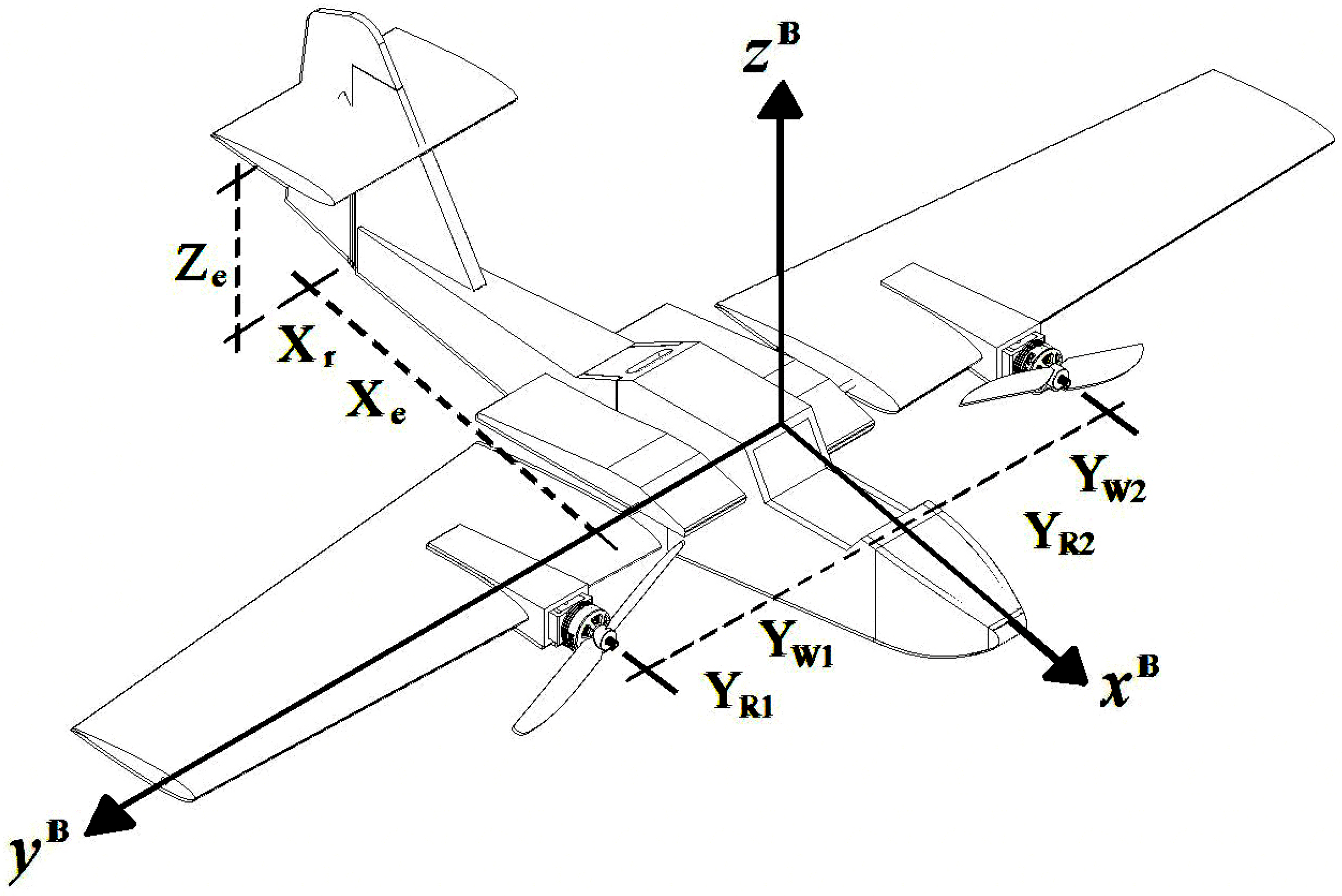
With , , , , as the distances on the X,Y axes of the forces acting on the vehicle of the rotors (R), wings (W), horizontal (e) and vertical (r) stabilizer respectively (Figure 3), the main moments are defined as follows:
The gyroscopic moment, with as the propeller inertia moment on its rotation axis and as the rotor angular velocity, is described as:
Finally, the drag moment, where is the propeller drag force, is defined as:
3. Parameters
This section is focused on obtaining the UAV’s physical parameters to be used for the simulation of the adopted altitude and attitude controllers.
3.1. Vehicle Mass
Because the vehicle’s thrust is generated by two rotors for vertical flight mode, the vehicle has to be lightweight and capable of withstanding the possible loadings in its different flight modes. Therefore, for the UAV construction, foam board is used for the fuselage, boom and landing gear, EPS for wings and vertical and horizontal stabilizer, with carbon fiber tubes in the wings as reinforcements. By the vehicle structure, electronic system, rotors and Li-Po battery, the vehicle total weight is 1 Kg.
3.2. Inertia Tensor
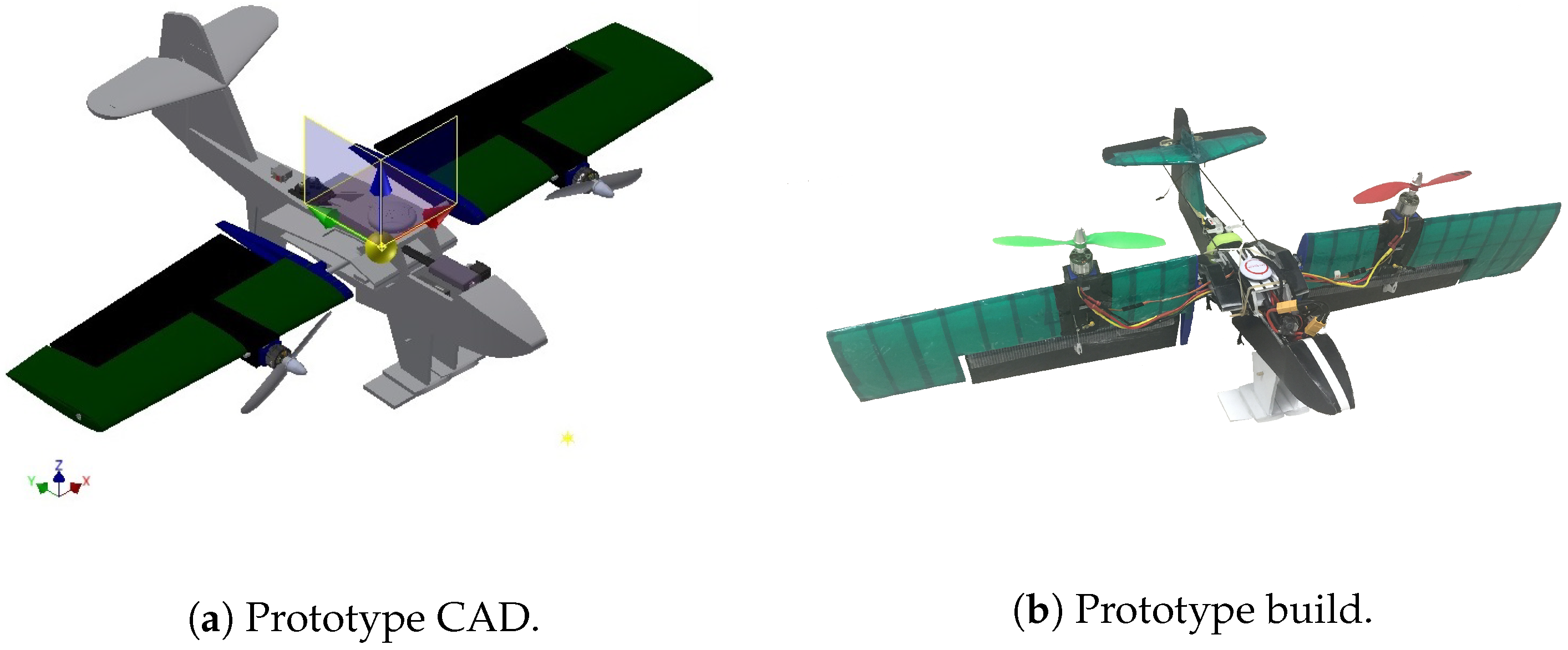
A Computer Aided Design (CAD) software, ©SolidWorks, is used to obtain the inertia tensor. Once the vehicle is designed, the proper material type is added to the different parts in the model so that the weight, mass center, and inertia tensor matrix could be estimated.
In order to make the mass center coincide with the aerodynamic center, both are positioned at 25% of the symmetrical profile’s chord of wing.
3.3. Aerodynamic Effects
During vertical flight, the wings and horizontal stabilizer generate aerodynamic effects that are included into the dynamic model.
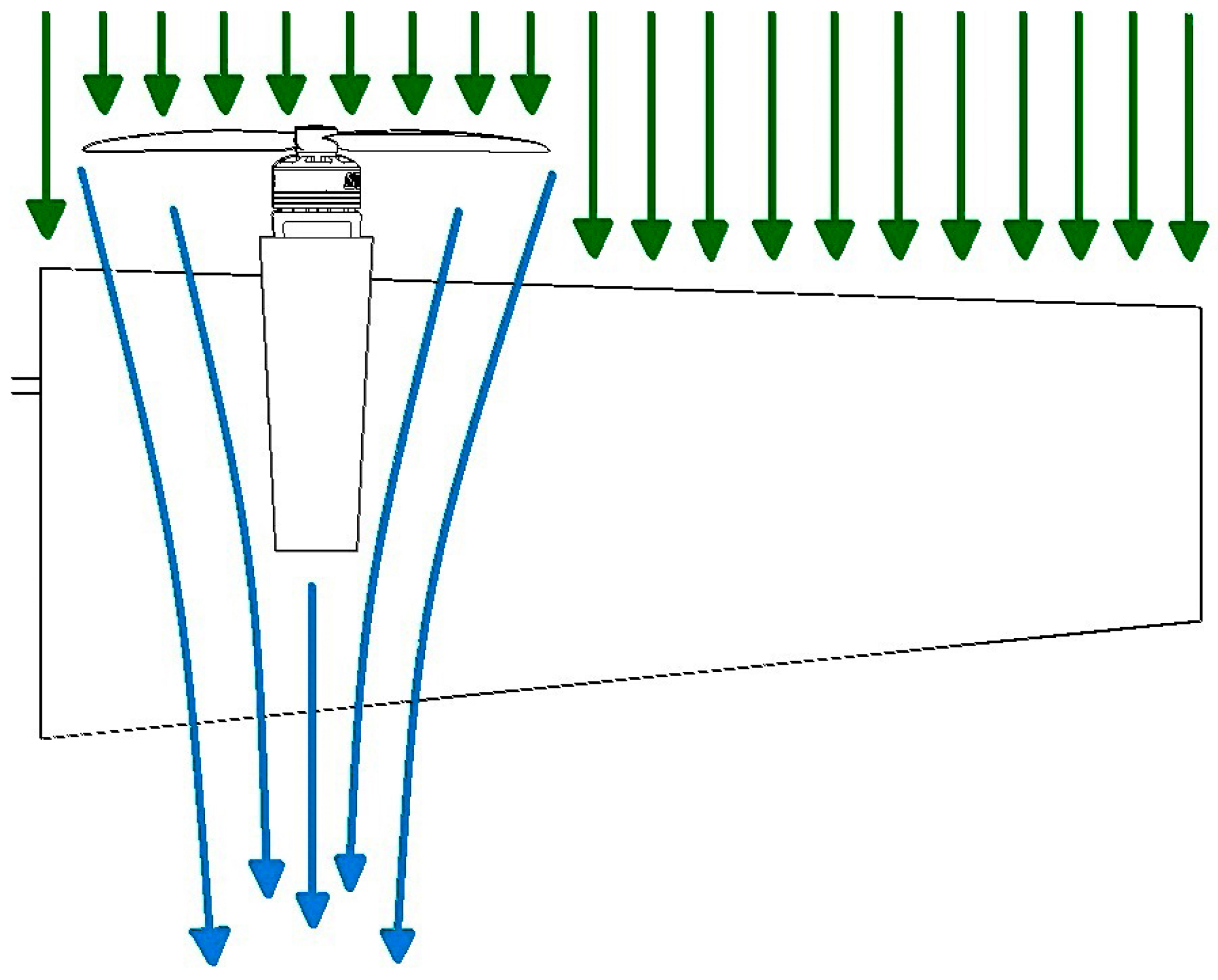
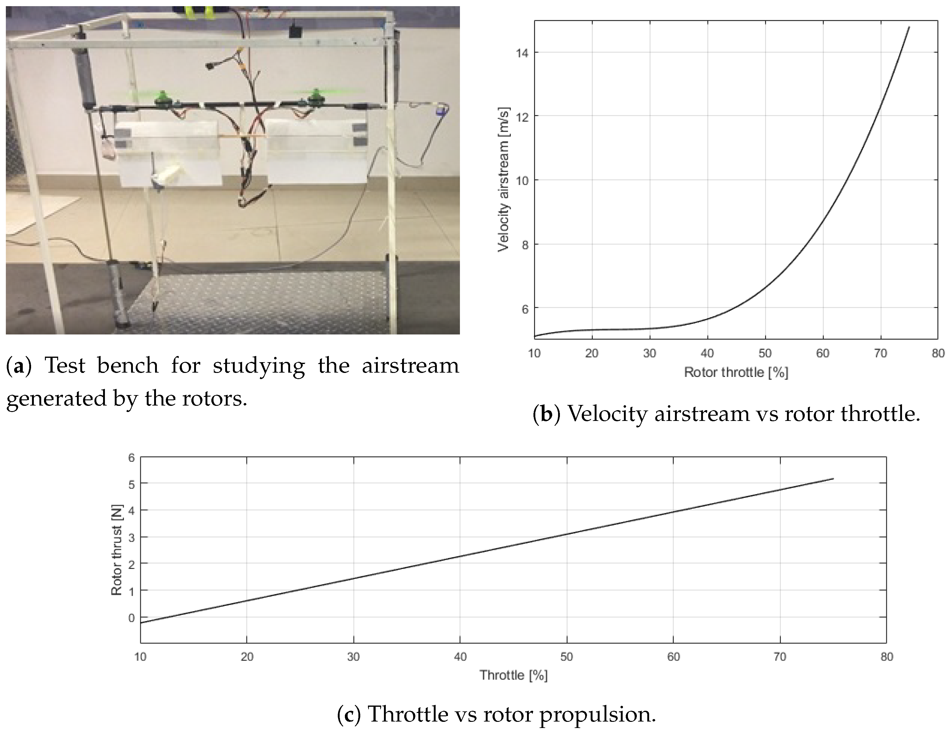
To study the aerodynamic effects on wing, a symmetrical airfoil (NACA 0012) is considered, knowing that the wing and rotors are tilting together, the airstream generated by the rotors is aligned with the wing chord line and due to incident airflow; the wing is divided into two areas, the wetted area which is in under the airstream generated by the rotors and the unwetted area with free stream (Figure 4). The aerodynamic of the free stream area has a major contribution to the aircraft’s lift. The wing area under the propeller, due to the profile used, the lift force and moment are canceled due to the symmetrical flow condition caused by the rotor, namely, does not generate lift but it generates drag and, therefore, subtracts thrust from rotors.
Firstly, the projected area on the wing that is affected by the airstream generated by the rotors is studied. Thus, a test bench is built (Figure 5a), where the wing and rotor are considered. Propellers “10 × 4.5” are used for the propulsion force, a pitot tube is located in the middle of the wing surface to determine the propeller airspeed with static thrust and to obtain the aerodynamic parameters such as the drag on the area under airstream generated by the rotors. Figure 5b shows the velocity airstream as a function of rotor’s throttle and Figure 5c shows the throttle as a function of rotor’s propulsion force.
With the maximum velocity airstream generated by the rotors obtained, 3D aerodynamic analysis is performed for this region. The UAV’s drag coefficient () is calculated by using Computational Fluid Dynamics method (CFD), using ©ANSYS fluent software. The drag force [18,19] is obtained by the following expression:
where is the air density, S the wing planform area, V the airflow velocity, the drag coefficient. Finally, the drag force is assumed as a polynomial function in terms of rotor’s propulsion force.
The drag force of the wing’s second section and horizontal stabilizer are a function of the rate of climb in vertical flight mode. Similarly, the drag coefficients are calculated by using CFD method and the drag forces by the Equation (13). A polynomial function in terms of the rate of climb for the wing’s drag force and the horizontal stabilizer is obtained. Using the same flight conditions and the same geometry of the aerodynamical configuration, the polynomial functions presented in this paper can be used in other research studies.
4. Results and Discussion
4.1. Controller Design for Validation
In this section, the complete mathematical model is validated. For simplicity, the UAV’s different flight dynamics are studied separately. First, the flight in VTOL mode is analyzed, therefore, the equations are simplified for VTOL flight mode conditions. Subsequently, PD controllers are adopted for altitude and attitude control and are tested in simulations and experiments.
Assumptions
- (A)
- For the vertical flight at , the thrust component is cos() and sin(), that is, the thrust is parallel to the Z-axis.
- (B)
- The x and y displacements are neglected because they are small compared to the z displacement (Altitude).
- (C)
- The wings and horizontal stabilizer do not generate lift forces as a function of the angle of attack (), only as a function of the control surfaces (only ailerons).
- (D)
- The vertical stabilizer does not generate aerodynamic effects.
- (E)
- Since gyroscopic effects on propellers are small enough, they are neglected.
- (F)
- The yaw () and roll () motions are small compared to pitch (), so that and .
From Equations (7) and (9), the resulting linearized altitude and attitude dynamics can be expressed in earth fixed inertial reference frame, as:
where is a virtual control input in terms of actuating forces and , and are a virtual control inputs in terms of actuating torques.
A PD controller [20] is adopted for altitude control and three PD controllers are adopted for attitude control. Controllers adopted are defined by the following equations:
4.2. Simulation
Numerical simulations validate the proposed complete dynamic model with aerodynamic effects considered. For simplicity and functionality, we have chosen to use a PD controller. The simulations are carried out in Matlab/Simulink environment.
Table 1 shows the operation range of UAV’s actuators. In Table 2 the parameters and the applicable dimensions to the vehicle are shown. Conditions of the simulation are shown in Table 3. Last, the control parameters obtained experimentally are shown in Table 4.
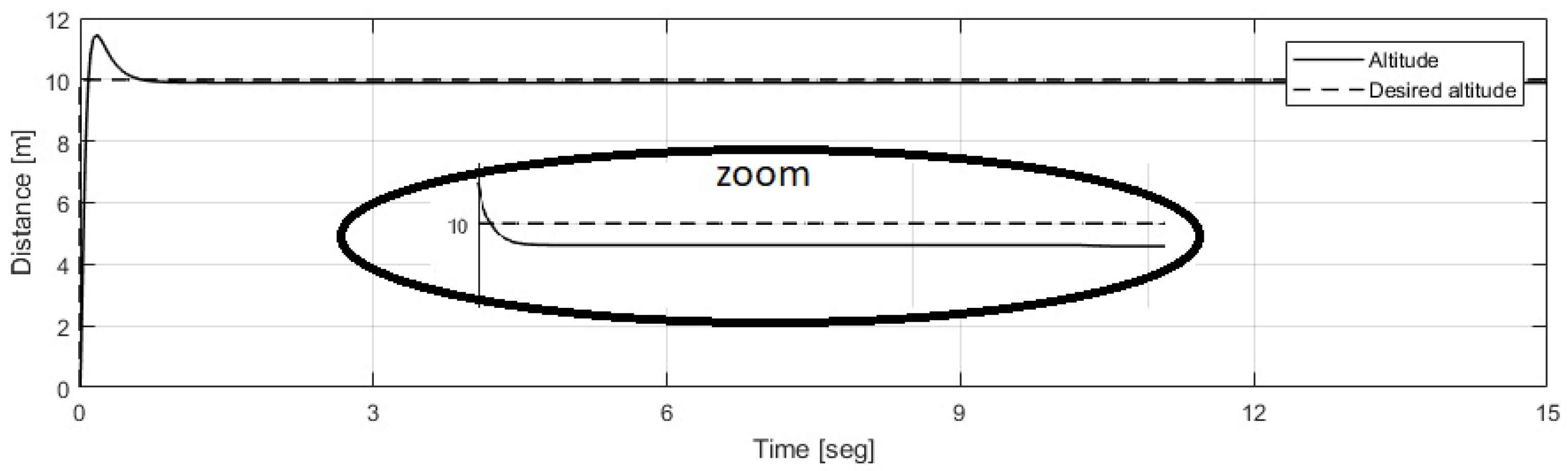
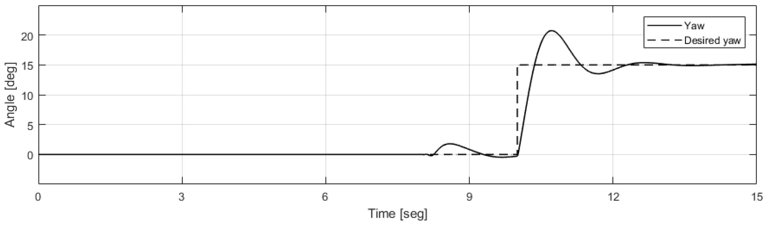
A vertical take-off, hover and landing scenario is considered. During the first 3 s, the vehicle takes off and climbs to 10 m. Then, at 5 s, the vehicle rotates on the X axis (Roll) to 15 degrees, later, at 8 s, the vehicle rotates on the Y axis (Pitch) to 15 degrees and at 10 s, the vehicle rotates on the Z axis (Yaw) to 15 degrees, preserving its altitude. Finally, the vehicle lands in 20 s.
Figure 6a,b shown the corresponding control signals to the motors (rotors) and servomotors (ailerons). Notice that during vertical take-off, each rotor generates approximately 5N at 60% throttle that compensate the vehicle’s weight and the drag forces of the wing and horizontal stabilizer. When the vehicle carries out a rotation motion (Roll, pitch, yaw), vertical component of thrust decreases, therefore, rotors thrust increase without exceeding its maximum capacity to preserving its altitude.
Also, notice that the UAV reached the desired altitude (Figure 7) while the error signals (Figure 8a,b) rapidly converge to the reference signal, without large overshots and oscillations despite using PD controllers. Even, after performing the roll (Figure 9), pitch (Figure 10) and Yaw (Figure 11) motions, is managed to perform a quick recovery of the system stability in only a second.
Figure 12 shows the drag obtained on the wing area affected with the airstream generated by the propeller that is included in the model. First, the drag increases because the motors increase their rotational speed to achieve the desired altitude, then, the drag decreases because the motors decrease their rotational speed because the vehicle exceeds the desired altitude and also due to the roll and pitch motion. Later, the drag is stabilized because the motors have the same rotation speed at the same desired flight altitude.
4.3. Flight Test in Real-Time
This section shows the real-time results of the vehicle’s flight tests to perform for vertical take-off, hover and landing.
Dual tilt-wing UAV is built as shown in Figure 13a,b. The main material used for construction is polyurethane foam for the wing and cardboard foam for the fuselage and empennage. Two motors with propelles “10 × 4.5” are mounted on the mid-span leading-edges of the wings.
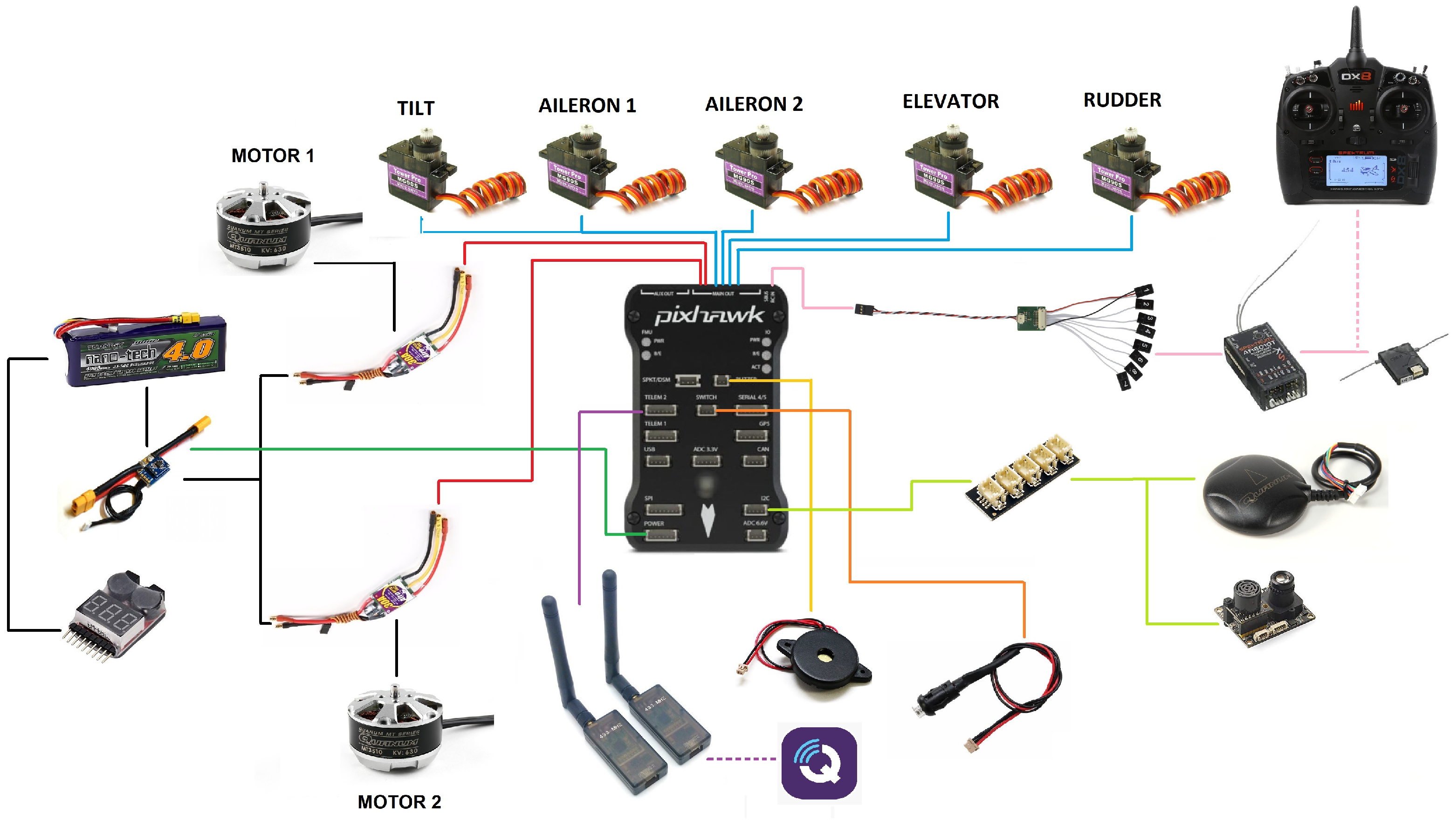
Figure 14 shows the UAV instrumentation, where two servo motors are for the ailerons, a servo motor for the elevator, a servo motor for the rudder and a servo motor for tilt mechanism. The PIXHAWK flight controller is used, roll and pitch angles are measured with an accelerometer, yaw with a magnetometer and altitude with a barometer. The electronic system is powered by a 40 Ah Lipo battery that is placed in the fuselage.
Flight tests outdoors were performed in Mexico City, at an altitude of 2250 m above the sea level. Since this paper focuses on vertical flight, the flight tests are only in VTOL mode.
For real-time flight tests, a scenario is considered in which the vehicle takes off in vertical mode until hovering, then rotation displacements are performed (roll, pitch and yaw), and finally, a vertical landing is carried out. The altitude is controlled using the throttle control. Roll, pitch and yaw angles are controlled manually, while the vehicle achieves a stable hovering.
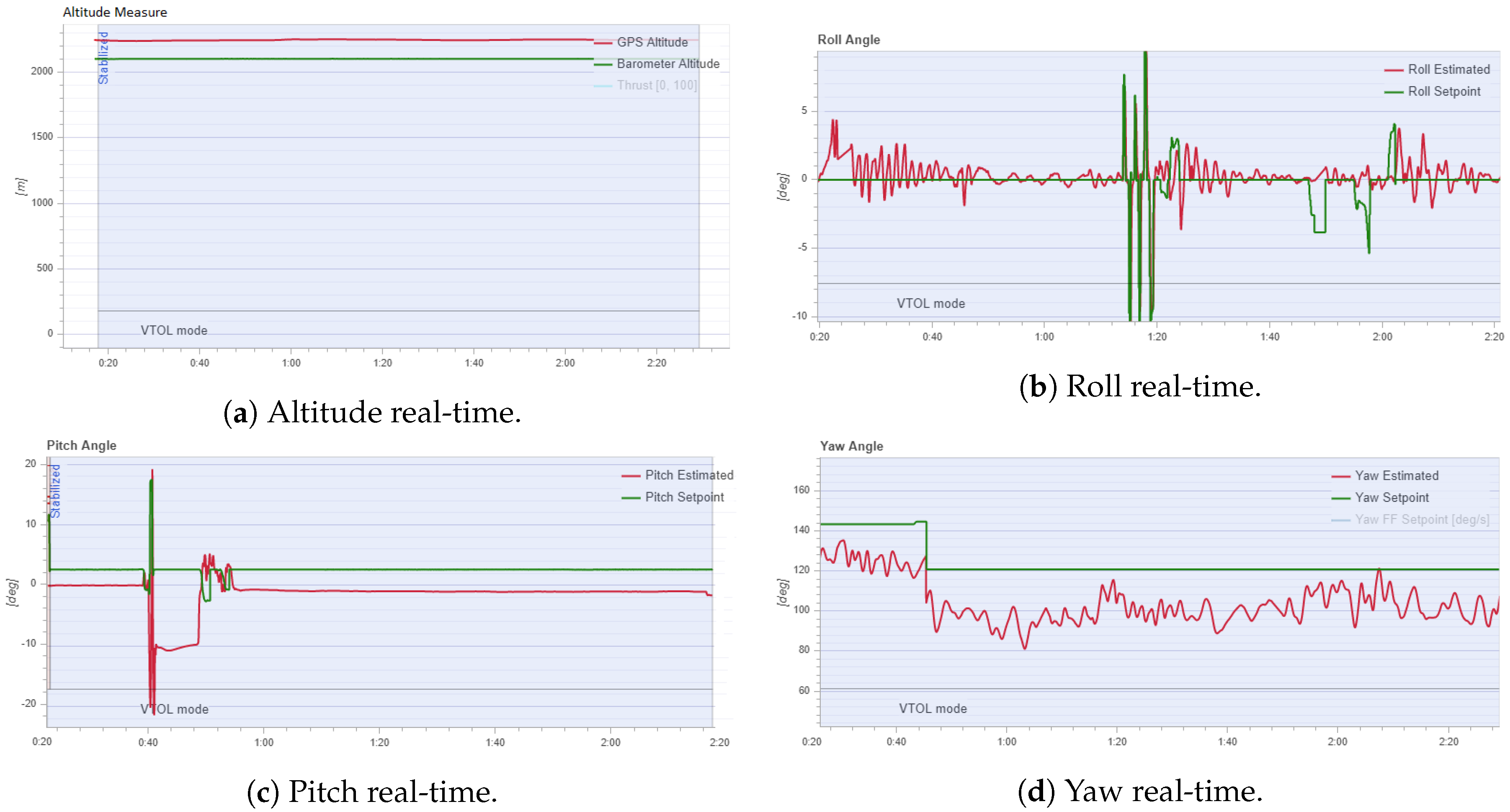
Figure 15a shows the altitude response, where results similar to the numerical simulation are obtained. Figure 15b–d shows the real-time responses of the vehicle orientation, roll, pitch and yaw, respectively. A stable hover flight was accomplished in which the control inputs (rotors and ailerons) never exceeded their constraints, despite the fact that the vehicle was perturbed by the wind.
The roll angle did not exceed its reference for more than 4 degrees, whereas the tracking error in yaw was bounded by 10 degrees. The pitch reference was kept at 8 degrees, although this reference is more difficult to stabilize.
5. Conclusions
In this paper, a Dual Tilt-wing is studied. The UAV complete dynamic model is obtained using the Newton–Euler formulation, aerodynamic effects are included on the wing and empennage as a function of the cruise speed, tilt angle and angle of attack. For aerodynamic analysis, the wing is divided into two sections, an area that is affected by airstream generated by the rotors and an area that is affected by the cruising speed. Experiments in a test bench and 3D simulations were performed to obtain the aerodynamic effects that are embedded to the model.
To validate the UAV dynamic model, PD controllers were adopted for altitude and attitude control of the vehicle in vertical flight mode. Numerical simulations and flight tests in real-time showed that the error signals rapidly converge to the reference signals, accomplishing stable flights in vertical mode.
As future work, the side wind effect on the wings in vertical flight mode will be included in the dynamic model. The model will be validated for the transition and horizontal flight modes, so that the three flight modes of the Dual Tilt-wing UAV can be studied with control approaches to improve the stability of the controlled system.
Author Contributions
Conceptualización, investigation, writing-original draft preparation, L.M.S.-R.; Methodology, writing–review and editing, R.L.; Software, formal analysis and supervision, A.A.-M. All authors have read and agreed to the published version of the manuscript.
Funding
This research was funded by CONACYT of Mexico through project 314879 “Laboratorio Nacional en Vehiculos Autonomos y Exoesqueletos LANAVEX”. The lead author was also supported by the UMI-LAFMIA CINVESTAV Mexico Preeminent Doctoral Program.
Conflicts of Interest
The authors declare no conflict of interest. The funders had no role in the design of the study; in the collection, analyses, or interpretation of data; in the writing of the manuscript, or in the decision to publish the results.
References
- Lindqvist, A.; Fresk, E.; Nikolakopoulos, G. Optimal Design and Modeling of a Tilt Wing Aircraft. In Proceedings of the 23rd Mediterranean Conference on Control and Automation, Torremolinos, Spain, 16–19 June 2015. [Google Scholar]
- Flores, G.; Escareño, J.; Lozano, R.; Salazar, S. Quad-Tilting Rotor Convertible MAV: Modeling and Real-Time Hover Flight Control. J. Intell. Robot. Syst. 2012, 65, 457–471. [Google Scholar] [CrossRef] [Green Version]
- Chen, C.; Zhang, J.; Zhang, D.; Shen, L. Control and flight test of a tilt-rotor unmanned aerial vehicle. Int. J. Adv. Robot. Syst. 2017, 14, 1–12. [Google Scholar] [CrossRef]
- Aktas, Y.O.; Ozdemir, U.; Dereli, Y.; Tarhan, A.F.; Cetin, A.; Vuruskan, A.; Yuksek, B.; Cengiz, H.; Basdemir, S.; Ucar, M.; et al. Rapid prototyping of a Fixed-Wing VTOL UAV for Design Testing. J. Intell. Robot. Syst. 2016, 84, 639–664. [Google Scholar] [CrossRef]
- Centinsoy, E.; Sirimoglu, E.; Oner, K.T.; Hancer, C.; Unel, M.; Aksit, M.F.; Kandemir, I.; Gulez, K. Design and development of a tilt-wing UAV. Turk. J. Electr. Eng. Comput. Sci. 2011, 19, 733–741. [Google Scholar]
- Sato, M.; Muraoka, K. Flight Controller Design and Demonstration of Quad-Tilt-Wing Unmanned Aerial Vehicle. J. Guid. Control Dyn. 2015, 38, 1–12. [Google Scholar] [CrossRef]
- Muraoka, K.; Okada, N.; Kubo, D. Quad Tilt Wing VTOL UAV: Aerodynamic Characteristics and Prototype Flight Test. In Proceedings of the AIAA Infotech@Aerospace Conference, Seattle, WA, USA, 6–9 April 2009. [Google Scholar]
- Small, E.; Fresk, E.; Andrikopoulos, G.; Nikolakopoulos, G. Modelling and Control of a Tilt-Wing Unmanned Aerial Vehicle. In Proceedings of the 24th Mediterranean Conference on Control and Automation, Athens, Greece, 21–24 June 2016. [Google Scholar]
- DHL Parcelcopter 3.0. Available online: https://www.dpdhl.com/en/media-relations/specials/dhl-parcelcopter.html (accessed on 10 October 2020).
- Benkhoud, K.; Bouallegue, S. Dynamics modeling and advanced metaheuristics based LQG controller design for a Quad Tilt Wing UAV. Int. J. Dyn. Control 2018, 6, 630–651. [Google Scholar] [CrossRef]
- Masuda, K.; Uchiyama, K. Robust control design for Quad Tilt-wing UAV. Aerospace 2018, 5, 17. [Google Scholar] [CrossRef] [Green Version]
- Cetinsoy, E.; Dikyar, S.; Hancer, C.; Oner, K.T.; Sirimoglu, E.; Unel, M.; Aksit, M.F. Design and construction of a novel quad tilt-wing UAV. Mechatronics 2012, 22, 723–745. [Google Scholar] [CrossRef]
- Garcia, O.; Castillo, P.; Wong, K.C.; Lozano, R. Attitude stabilization with real-time experiments of a tail-sitter aircraft in horizontal flight. J. Intell. Robot. Syst. 2012, 65, 123–136. [Google Scholar] [CrossRef] [Green Version]
- Takeuchi, R.; Watanabe, K.; Nagai, I. Development and control of tilt-wings for a tilt-type Quadrotor. In Proceedings of the IEEE International Conference on Mechatronics and Automation, Takamatsu, Japan, 6–9 August 2017. [Google Scholar]
- Etkin, B.; Reid, L.D. Dynamics of Flight: Stability and Control, 3rd ed.; John Wiley & Sons, Inc.: Hoboken, NJ, USA, 1996. [Google Scholar]
- Cook, M.V. Flight Dynamics Principles: A Linear Systems Approach to Aircraft Stability and Control, 3rd ed.; Elsevier Ltd.: New York, NY, USA, 2013. [Google Scholar]
- Escareño, J.; Salazar, S.; Lozano, R. Modelling and control of a convertible VTOL aircraft. In Proceedings of the IEEE Conference on Decision & Control, San Diego, CA, USA, 13–15 December 2006. [Google Scholar]
- Abbott, I.H.; Doenhoff, A.E.V. Theory of Wing Sections; Dover Publications, Inc.: New York, NY, USA, 1959. [Google Scholar]
- Anderson, J.D., Jr. Fundamentals of Aerodynamics, 5th ed.; McGraw-Hill: New York, NY, USA, 2011. [Google Scholar]
- Oner, K.T.; Cetinsoy, E.; Sirimoglu, E.; Hancer, C.; Unel, M.; Aksit, M.F.; Gulez, K.; Kandemir, I. Mathematical modeling and vertical flight control of a tilt-wing UAV. Turk. J. Electr. Eng. Comput. Sci. 2012, 20, 149–157. [Google Scholar]
Figure 1.
Unmanned Aerial Vehicles (UAV) motion variables notation.

Figure 2.
Aerodynamic forces and controls notation.

Figure 3.
Distances of the forces acting on the UAV.

Figure 4.
Airstream on the wing.

Figure 5.
Aerodynamic effects of the area on the wing that is affected by the airstream generated by the rotors.
Figure 5.
Aerodynamic effects of the area on the wing that is affected by the airstream generated by the rotors.

Figure 6.
Responses of controllers.

Figure 7.
Altitude control response.

Figure 8.
Error signals.

Figure 9.
Roll angle and control.

Figure 10.
Pitch angle and control.

Figure 11.
Yaw angle and control.

Figure 12.
Aerodynamic drag force.

Figure 13.
Dual tilt-wing UAV prototype.

Figure 14.
UAV electronic instrumentation.

Figure 15.
Flight test results in real-time.


Table 1.
Operation range of actuators.
| Parameter | Value | Unit |
|---|---|---|
| Propeller thrust | (n = 1, 2) | N |
| Aileron angle | (n = 1, 2) | rad |
| Tilt angle | (n = 1, 2) | rad |
Table 2.
Parameters.
| Parameter | Value | Unit |
|---|---|---|
| m | 1 | kg |
| g | 9.80665 | m/s2 |
| 0.024 | Kg·m2 | |
| 0.010 | Kg·m2 | |
| 0.033 | Kg·m2 | |
| 0.25 | m | |
| 0.25 | m | |
| 1.225 | Kg/m3 | |
| S | 0.08 | m2 |
Table 3.
Simulation conditions.
| Parameter | Value | Unit | |
|---|---|---|---|
| Velocity initial | m/s | ||
| Angular velocity initial | rad/s | ||
| Attitude initial | rad | ||
| Target position | (Time ≤ 3 s) | m | |
| (Time = 5 s) | rad | ||
| (Time = 8 s) | rad | ||
| (Time = 10 s) | rad |
Table 4.
Control parameters.
| K | Roll | Pitch | Yaw | Altitude |
|---|---|---|---|---|
| 0.21 | 0.21 | 0.4 | 100 | |
| 0.055 | 0.105 | 0.09 | 20 |
Publisher’s Note: MDPI stays neutral with regard to jurisdictional claims in published maps and institutional affiliations. |
© 2020 by the authors. Licensee MDPI, Basel, Switzerland. This article is an open access article distributed under the terms and conditions of the Creative Commons Attribution (CC BY) license (http://creativecommons.org/licenses/by/4.0/).
Share and Cite
MDPI and ACS Style
Sanchez-Rivera, L.M.; Lozano, R.; Arias-Montano, A. Development, Modeling and Control of a Dual Tilt-Wing UAV in Vertical Flight. Drones 2020, 4, 71. https://0-doi-org.brum.beds.ac.uk/10.3390/drones4040071
AMA Style
Sanchez-Rivera LM, Lozano R, Arias-Montano A. Development, Modeling and Control of a Dual Tilt-Wing UAV in Vertical Flight. Drones. 2020; 4(4):71. https://0-doi-org.brum.beds.ac.uk/10.3390/drones4040071
Chicago/Turabian StyleSanchez-Rivera, Luz M., Rogelio Lozano, and Alfredo Arias-Montano. 2020. "Development, Modeling and Control of a Dual Tilt-Wing UAV in Vertical Flight" Drones 4, no. 4: 71. https://0-doi-org.brum.beds.ac.uk/10.3390/drones4040071