The Methodological Aspects of Constructing a High-Resolution DEM of Large Territories Using Low-Cost UAVs on the Example of the Sarycum Aeolian Complex, Dagestan, Russia


Abstract
:1. Introduction
2. Materials and Methods
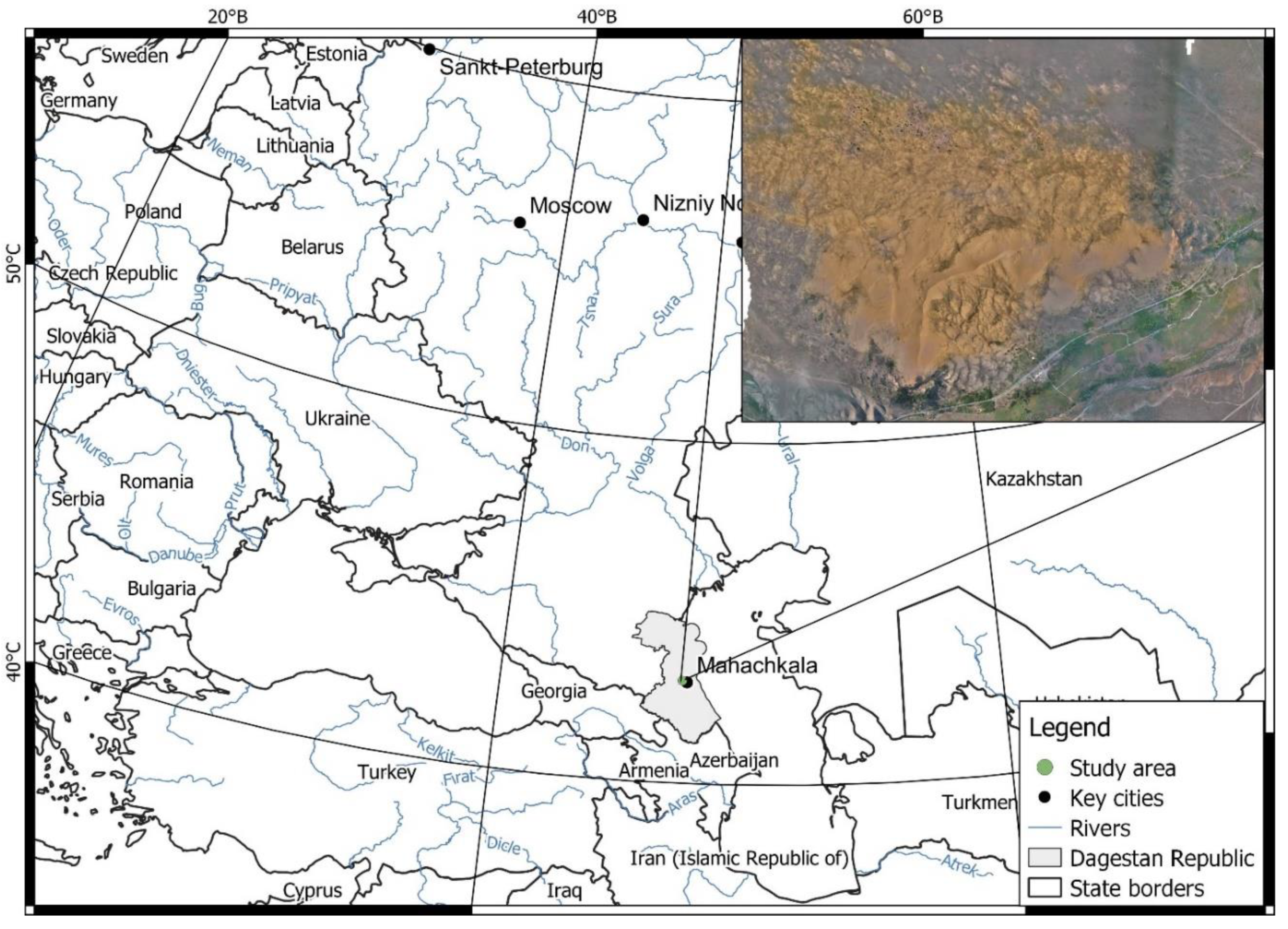
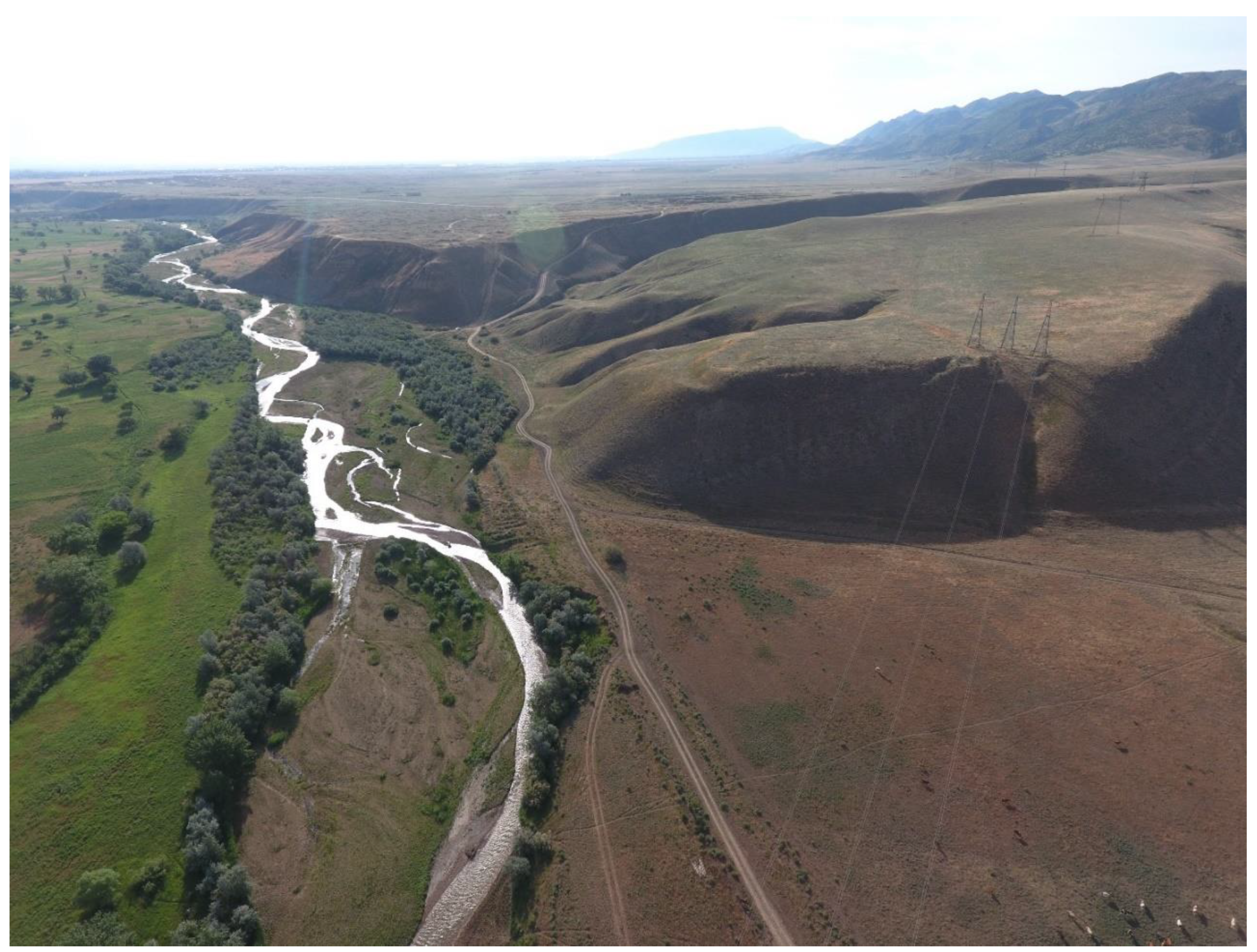
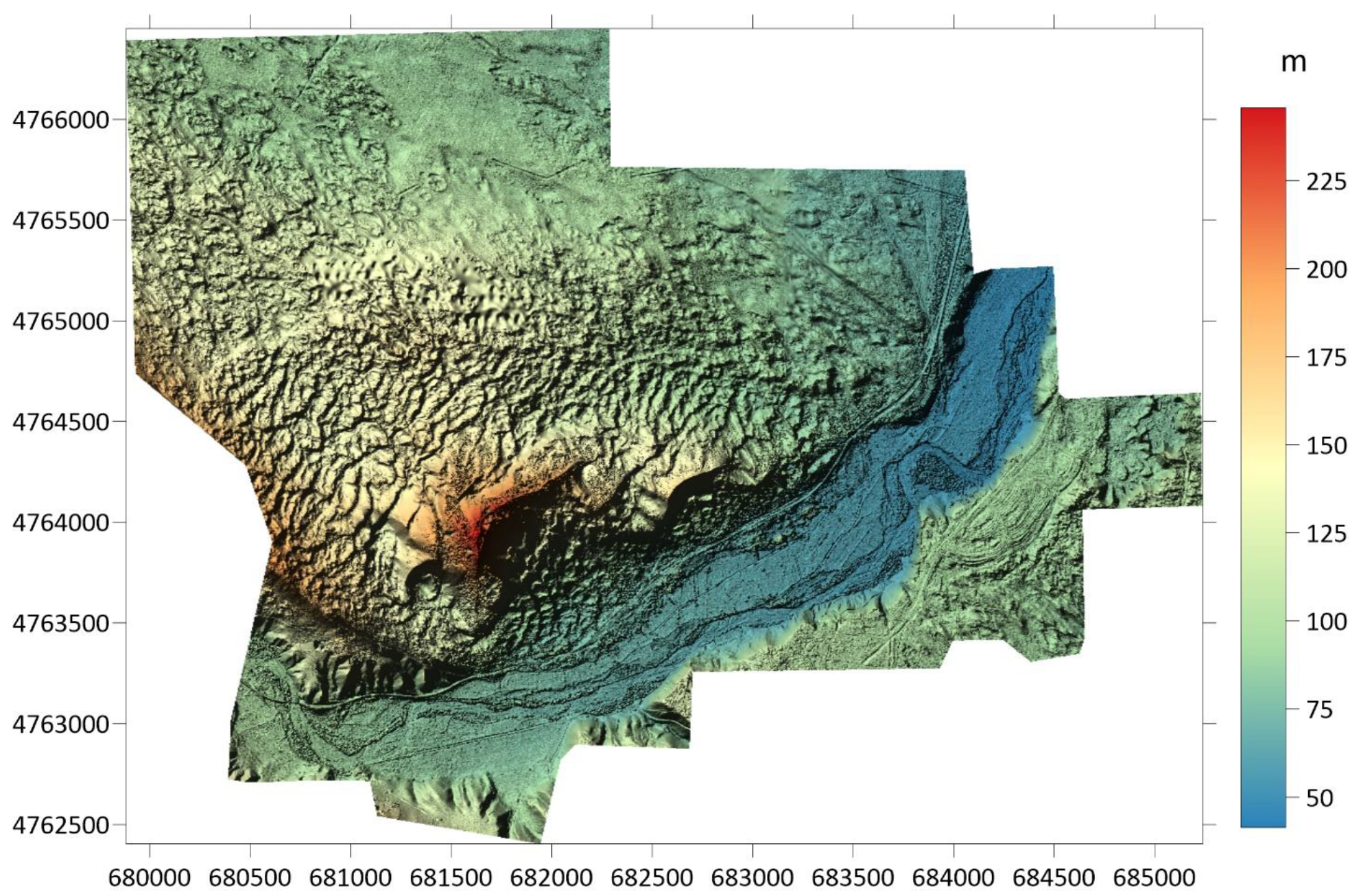
2.1. Study Area
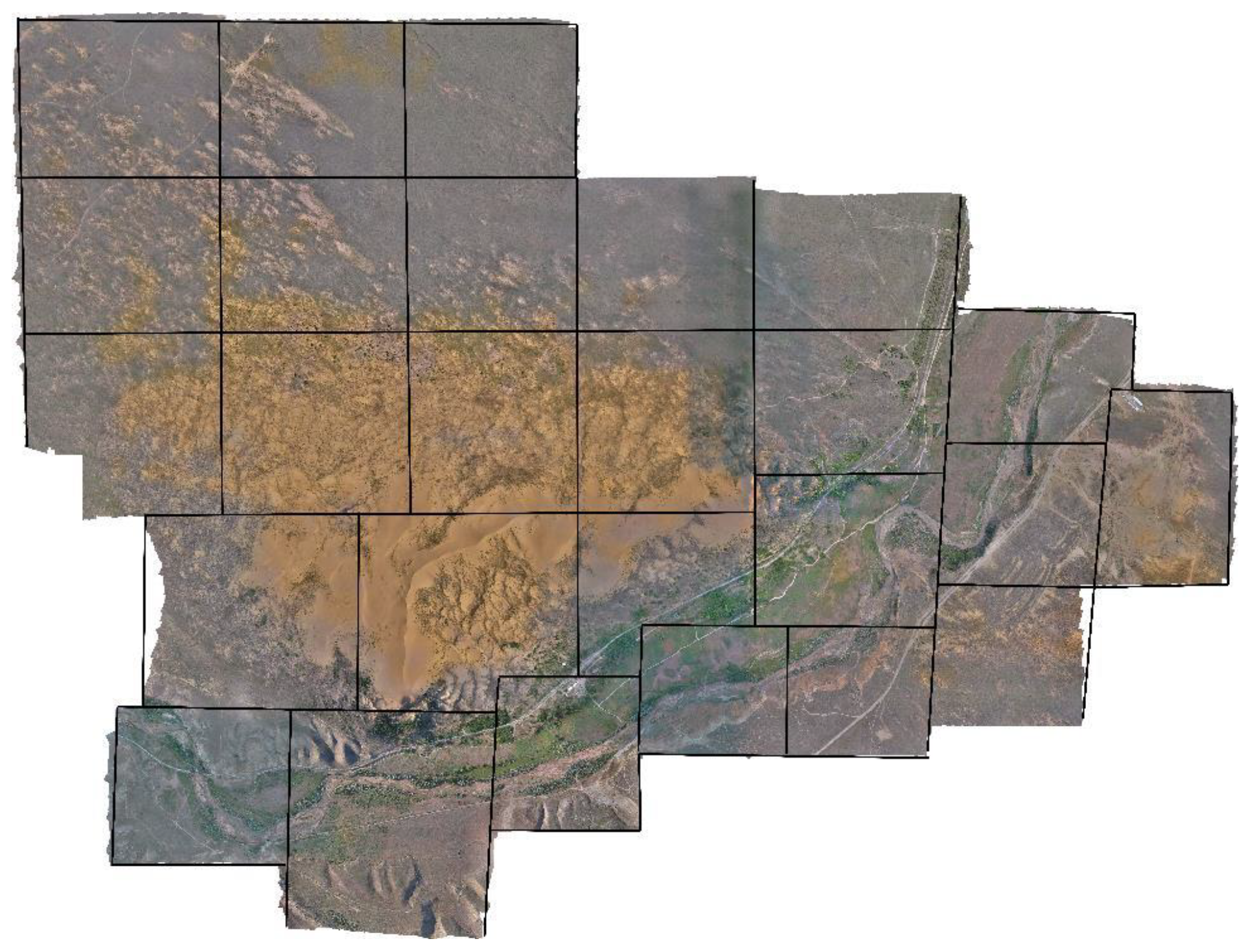
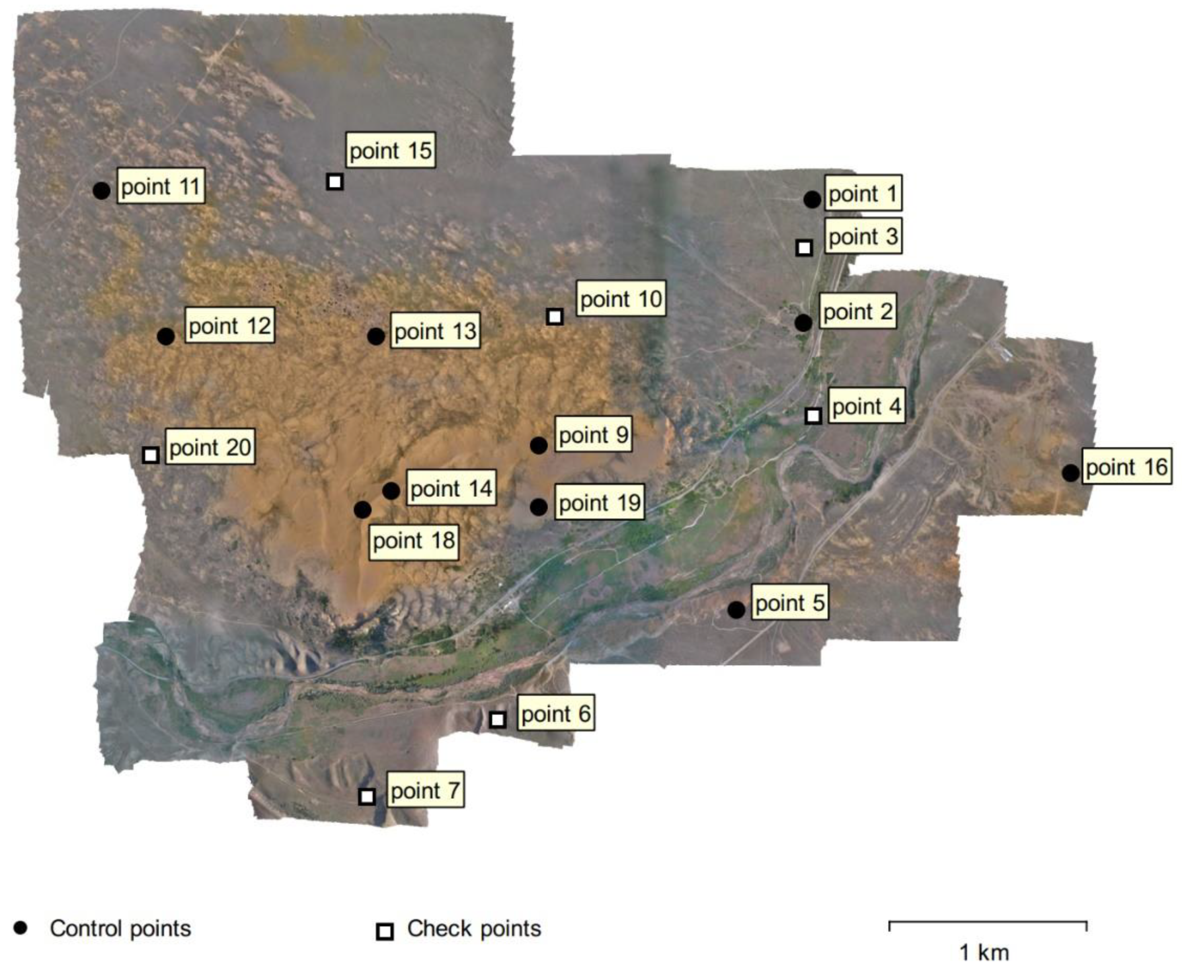
2.2. Field Research Methodology
3. Results and Discussion
- The texture of the survey surface. Since June in Dagestan is characterized by hot and scorching sun, with usually zero cloudiness, aeolian forms, namely sands, create inconstant glare. In addition, the texture is extremely uniform in places. All these factors lead to the fact that the number of common points in the images tends to zero, and in places where it was still possible to detect a sufficient number of common points, there are specific noises and outliers in the dense point cloud. As a solution to this problem, it makes sense to increase the camera angle, which was described earlier.
- Difficult terrain. Since the altitude difference in the study area is 197 m, starting flight missions from one point becomes impossible, since the overlap of neighboring images decreases with increasing terrain height. In this case, there are no options other than to launch UAVs from the dune slopes and flat areas of the foothills.
- The hardware and software capabilities are undeveloped. In 2017, the DJI Phantom 4, in combination with Pix4D Capture, made it possible to survey small objects. The hardware and software capabilities differed depending on the operating system of the smartphone, but the basic principle remained the same. In 2020, much more advanced software features appeared, including taking into account terrain features when calculating flight altitude and overlapping images, as well as RTK solutions for the DJI Phantom 4. All of this would allow for a qualitatively different level of work; however, the cost of modifying the DJI Phantom 4 reduces its price appeal. Returning to the software, it is necessary to note that creation of the project for surveying a large territory “squares” is still not provided by software developers, so the only option for planning work of this extent is still either a manual survey or preparation of a series of kml or shp-files with borders of “squares” of interest in the GIS.
4. Conclusions
Funding
Institutional Review Board Statement
Informed Consent Statement
Data Availability Statement
Conflicts of Interest
References
- Day, S.S.; Gran, K.B.; Belmont, P.; Wawrzyniec, T. Measuring Bluff Erosion Part 2: Pairing Aerial Photographs and Terrestrial Laser Scanning to Create a Watershed Scale Sediment Budget. Earth Surf. Process. Landf. 2013, 38, 1068–1082. [Google Scholar] [CrossRef]
- Calligaro, S.; Sofia, G.; Prosdocimi, M.; Fontana, G.D.; Tarolli, P. Terrestrial laser scanner data to support coastal erosion analysis: The conero case study. ISPRS Int. Arch. Photogramm. Remote Sens. Spat. Inf. Sci. 2014, 5, 125–129. [Google Scholar] [CrossRef] [Green Version]
- Goodwin, N.R.; Armston, J.; Stiller, I.; Muir, J. Assessing the Repeatability of Terrestrial Laser Scanning for Monitoring Gully Topography: A Case Study from Aratula, Queensland, Australia. Geomorphology 2016, 262, 24–36. [Google Scholar] [CrossRef]
- Drăguţ, L.; Eisank, C. Automated Object-Based Classification of Topography from SRTM Data. Geomorphology 2012, 141, 21–33. [Google Scholar] [CrossRef] [PubMed] [Green Version]
- Bouaziz, M.; Wijaya, A.; Gloaguen, R. Remote Gully Erosion Mapping Using Aster Data and Geomorphologic Analysis in the Main Ethiopian Rift. Geo Spat. Inf. Sci. 2011, 14, 246–254. [Google Scholar] [CrossRef]
- Suwandana, E.; Kawamura, K.; Sakuno, Y.; Kustiyanto, E.; Raharjo, B. Evaluation of ASTER GDEM2 in Comparison with GDEM1, SRTM DEM and Topographic-Map-Derived DEM Using Inundation Area Analysis and RTK-DGPS Data. Remote Sens. 2012, 4, 2419–2431. [Google Scholar] [CrossRef] [Green Version]
- Gesch, D.; Oimoen, M.; Danielson, J.; Meyer, D. Validation of the aster global digital elevation model version 3 over the conterminous united states. ISPRS Int. Arch. Photogramm. Remote Sens. Spat. Inf. Sci. 2016, 41, 143–148. [Google Scholar] [CrossRef]
- Ludwig, R.; Schneider, P. Validation of Digital Elevation Models from SRTM X-SAR for Applications in Hydrologic Modeling. ISPRS J. Photogramm. Remote Sens. 2006, 60, 339–358. [Google Scholar] [CrossRef]
- Chang, H.-C.; Ge, L.; Rizos, C.; Milne, T. Validation of DEMs Derived from Radar Interferometry, Airborne Laser Scanning and Photogrammetry by Using GPS-RTK. In Proceedings of the IEEE International Geoscience and Remote Sensing Symposium, Anchorage, AK, USA, 20–24 September 2004; Volume 5, pp. 2815–2818. [Google Scholar]
- Gafurov, A.M. Possible Use of Unmanned Aerial Vehicle for Soil Erosion Assessment. Uchenye Zap. Kazan. Univ. Seriya Estestv. Nauki 2017, 159, 654–667. [Google Scholar]
- Gafurov, A.M. Small Catchments DEM Creation Using Unmanned Aerial Vehicles. IOP Conf. Ser. Earth Environ. Sci. 2018, 107, 012005. [Google Scholar] [CrossRef]
- Frankenberger, J.R.; Huang, C.; Nouwakpo, K. Low-Altitude Digital Photogrammetry Technique to Assess Ephemeral Gully Erosion. In Proceedings of the IEEE International Geoscience and Remote Sensing Symposium, Boston, MA, USA, 7–11 July 2008; Volume 4, pp. 117–120. [Google Scholar]
- Walter, M.; Niethammer, U.; Rothmund, S.; Joswig, M. Joint Analysis of the Super-Sauze (French Alps) Mudslide by Nanoseismic Monitoring and UAV-Based Remote Sensing. Surf. Geosci. 2009, 27, 53–60. [Google Scholar]
- Agisoft Photoscan. Available online: http://www.agisoft.com/about/ (accessed on 7 February 2018).
- OpenCV Library. Available online: https://opencv.org/ (accessed on 7 February 2018).
- D’Oleire-Oltmanns, S.; Marzolff, I.; Peter, K.D.; Ries, J.B.; Hssaïne, A.A. Monitoring Soil Erosion in the Souss Basin, Morocco, with a Multiscale Object-Based Remote Sensing Approach Using UAV and Satellite Data. In Proceedings of the 1st World Sustainability Forum, Online, 1–30 November 2011; pp. 1–13. [Google Scholar]
- D’Oleire-Oltmanns, S.; Marzolff, I.; Peter, K.; Ries, J. Unmanned Aerial Vehicle (UAV) for Monitoring Soil Erosion in Morocco. Remote Sens. 2012, 4, 3390–3416. [Google Scholar] [CrossRef] [Green Version]
- Fritz, A.; Kattenborn, T.; Koch, B. UAV-Based Photogrammetric Point Clouds—Tree Stem Mapping in Open Stands in Comparison to Terrestrial Laser Scanner Point Clouds. ISPRS Int. Arch. Photogramm. Remote Sens. Spat. Inf. Sci. 2013, 40, 141–146. [Google Scholar] [CrossRef] [Green Version]
- Vasuki, Y.; Holden, E.-J.; Kovesi, P.; Micklethwaite, S. Semi-Automatic Mapping of Geological Structures Using UAV-Based Photogrammetric Data: An Image Analysis Approach. Comput. Geosci. 2014, 69, 22–32. [Google Scholar] [CrossRef]
- Gruszczyński, W.; Matwij, W.; Ćwiąkała, P. Comparison of Low-Altitude UAV Photogrammetry with Terrestrial Laser Scanning as Data-Source Methods for Terrain Covered in Low Vegetation. ISPRS J. Photogramm. Remote Sens. 2017, 126, 168–179. [Google Scholar] [CrossRef]
- Eltner, A.; Mulsow, C.; Maas, H.-G. Quantitative Measurement of Soil Erosion from TLS and UAV Data. ISPRS Int. Arch. Photogramm. Remote Sens. Spat. Inf. Sci. 2013, 40, 119–124. [Google Scholar] [CrossRef] [Green Version]
- Chetverikov, D.; Svirko, D.; Stepanov, D.; Krsek, P. The Trimmed Iterative Closest Point Algorithm. In Proceedings of the Object Recognition Supported by User Interaction for Service Robots, Quebec City, QC, Canada, 11–15 August 2002; Volume 3, pp. 545–548. [Google Scholar]
- Bouaziz, S.; Tagliasacchi, A.; Pauly, M. Sparse Iterative Closest Point. In Proceedings of the Proceedings of the Eleventh Eurographics/ACMSIGGRAPH Symposium on Geometry Processing; Eurographics Association: Goslar, Germany, 2013; pp. 113–123. [Google Scholar]
- Mancini, F.; Dubbini, M.; Gattelli, M.; Stecchi, F.; Fabbri, S.; Gabbianelli, G. Using Unmanned Aerial Vehicles (UAV) for High-Resolution Reconstruction of Topography: The Structure from Motion Approach on Coastal Environments. Remote Sens. 2013, 5, 6880–6898. [Google Scholar] [CrossRef] [Green Version]
- Zhang, R.; Schneider, D.; Strauß, B. Generation and comparison of TLS and SFM based 3d models of solid shapes in hydromechanic research. ISPRS Int. Arch. Photogramm. Remote Sens. Spat. Inf. Sci. 2016, 41, 925–929. [Google Scholar] [CrossRef]
- Nouwakpo, S.K.; Weltz, M.A.; McGwire, K. Assessing the Performance of Structure-from-Motion Photogrammetry and Terrestrial LiDAR for Reconstructing Soil Surface Microtopography of Naturally Vegetated Plots. Earth Surf. Process. Landf. 2016, 41, 308–322. [Google Scholar] [CrossRef]
- Wilkinson, M.W.; Jones, R.R.; Woods, C.E.; Gilment, S.R.; McCaffrey, K.J.W.; Kokkalas, S.; Long, J.J. A Comparison of Terrestrial Laser Scanning and Structure-from-Motion Photogrammetry as Methods for Digital Outcrop Acquisition. Geosphere 2016, 12, 1865–1880. [Google Scholar] [CrossRef] [Green Version]
- Richter, N.; Favalli, M.; de Zeeuw-van Dalfsen, E.; Fornaciai, A.; da Silva, F.R.M.; Pérez, N.M.; Levy, J.; Victória, S.S.; Walter, T.R. Lava Flow Hazard at Fogo Volcano, Cabo Verde, before and after the 2014-2015 Eruption. Nat. Hazards Earth Syst. Sci. 2016, 16, 1925–1951. [Google Scholar] [CrossRef] [Green Version]
- Müller, D.; Walter, T.R.; Schöpa, A.; Witt, T.; Steinke, B.; Gudmundsson, M.T.; Dürig, T. High-Resolution Digital Elevation Modeling from TLS and UAV Campaign Reveals Structural Complexity at the 2014/2015 Holuhraun Eruption Site, Iceland. Front. Earth Sci. 2017, 5, 59. [Google Scholar] [CrossRef] [Green Version]
- Lucieer, A.; Turner, D.; King, D.H.; Robinson, S.A. Using an Unmanned Aerial Vehicle (UAV) to Capture Micro-Topography of Antarctic Moss Beds. Int. J. Appl. Earth Obs. Geoinf. 2014, 27, 53–62. [Google Scholar] [CrossRef] [Green Version]
- Cawood, A.J.; Bond, C.E.; Howell, J.A.; Butler, R.W.H.; Totake, Y. LiDAR, UAV or Compass-Clinometer? Accuracy, Coverage and the Effects on Structural Models. J. Struct. Geol. 2017, 98, 67–82. [Google Scholar] [CrossRef]
- Schonberger, J.L.; Frahm, J.-M. Structure-from-Motion Revisited. In Proceedings of the 2016 IEEE Conference on Computer Vision and Pattern Recognition (CVPR), Las Vegas, NV, USA, 26 June 2016; pp. 4104–4113. [Google Scholar]
- Benassi, F.; Dall’Asta, E.; Diotri, F.; Forlani, G.; di Cella, U.M.; Roncella, R.; Santise, M. Testing Accuracy and Repeatability of UAV Blocks Oriented with GNSS-Supported Aerial Triangulation. Remote Sens. 2017, 9, 172. [Google Scholar] [CrossRef] [Green Version]
- Gindraux, S.; Boesch, R.; Farinotti, D. Accuracy Assessment of Digital Surface Models from Unmanned Aerial Vehicles’ Imagery on Glaciers. Remote Sens. 2017, 9, 186. [Google Scholar] [CrossRef] [Green Version]
- James, M.R.; Robson, S. Mitigating Systematic Error in Topographic Models Derived from UAV and Ground-Based Image Networks. Earth Surf. Process. Landf. 2014, 39, 1413–1420. [Google Scholar] [CrossRef] [Green Version]
- Uysal, M.; Toprak, A.S.; Polat, N. DEM Generation with UAV Photogrammetry and Accuracy Analysis in Sahitler Hill. Measurement 2015, 73, 539–543. [Google Scholar] [CrossRef]
- Udin, W.S.; Ahmad, A. Assessment of Photogrammetric Mapping Accuracy Based on Variation Flying Altitude Using Unmanned Aerial Vehicle. IOP Conf. Ser. Earth Environ. Sci. 2014, 18, 1–7. [Google Scholar] [CrossRef]
- Turner, D.; Lucieer, A.; Watson, C. An Automated Technique for Generating Georectified Mosaics from Ultra-High Resolution Unmanned Aerial Vehicle (UAV) Imagery, Based on Structure from Motion (SfM) Point Clouds. Remote Sens. 2012, 4, 1392–1410. [Google Scholar] [CrossRef] [Green Version]
- Agüera-Vega, F.; Carvajal-Ramírez, F.; Martínez-Carricondo, P.; Sánchez-Hermosilla, L.J.; Mesas-Carrascosa, F.J.; García-Ferrer, A.; Pérez-Porras, F.J. Reconstruction of Extreme Topography from UAV Structure from Motion Photogrammetry. Measurement 2018, 121, 127–138. [Google Scholar] [CrossRef]
- Boon, M.A.; Drijfhout, A.P.; Tesfamichael, S. Comparison of a Fixed-Wing and Multi-Rotor Uav for Environmental Mapping Applications: A Case Study. Int. Arch. Photogramm. Remote Sens. Spat. Inf. Sci. 2017, 42, 47. [Google Scholar] [CrossRef] [Green Version]
- Ajayi, O.G.; Salubi, A.A.; Angbas, A.F.; Odigure, M.G. Generation of Accurate Digital Elevation Models from UAV Acquired Low Percentage Overlapping Images. Int. J. Remote Sens. 2017, 38, 3113–3134. [Google Scholar] [CrossRef]
- Akturk, E.; Altunel, A.O. Accuracy Assessment of a Low-Cost UAV Derived Digital Elevation Model (DEM) in a Highly Broken and Vegetated Terrain. Measurement 2019, 136, 382–386. [Google Scholar] [CrossRef]
- Blistan, P.; Kovanič, L.; Patera, M.; Hurčík, T. Evaluation Quality Parameters of DEM Generated with Low-Cost UAV Photogrammetry and Structure-from-Motion (SfM) Approach for Topographic Surveying of Small Areas. Acta Montan. Slovaca 2019, 24, 198–212. [Google Scholar]
- Kurkov, V.M.; Kiseleva, A.S. DEM Accuracy Research Based on Unmanned Aerial Survey Data. Int. Arch. Photogramm. Remote Sens. Spat. Inf. Sci. 2020, 43, 1347–1352. [Google Scholar] [CrossRef]
- Taddia, Y.; Stecchi, F.; Pellegrinelli, A. Using DJI phantom 4 RTK drone for topographic mapping of coastal areas. Int. Arch. Photogramm. Remote Sens. Spat. Inf. Sci. 2019. [Google Scholar] [CrossRef] [Green Version]
- Zimmerman, T.; Jansen, K.; Miller, J. Analysis of UAS Flight Altitude and Ground Control Point Parameters on DEM Accuracy along a Complex, Developed Coastline. Remote Sens. 2020, 12, 2305. [Google Scholar] [CrossRef]
- Gaffey, C.; Bhardwaj, A. Applications of Unmanned Aerial Vehicles in Cryosphere: Latest Advances and Prospects. Remote Sens. 2020, 12, 948. [Google Scholar] [CrossRef] [Green Version]
- Gusarov, A.V.; Sharifullin, A.G.; Dzhamirzoev, G.S. The Contemporary Height of Aeolian Accumulative Complex Sarykum (Republic of Dagestan) and the Causes of Its Change. Izv. Ross. Akad. Nauk Seriya Geogr. 2017, 89–98. [Google Scholar] [CrossRef]
- Agüera-Vega, F.; Carvajal-Ramírez, F.; Martínez-Carricondo, P. Assessment of Photogrammetric Mapping Accuracy Based on Variation Ground Control Points Number Using Unmanned Aerial Vehicle. Measurement 2017, 98, 221–227. [Google Scholar] [CrossRef]
- James, M.R.; Robson, S.; D’Oleire-Oltmanns, S.; Niethammer, U. Optimising UAV Topographic Surveys Processed with Structure-from-Motion: Ground Control Quality, Quantity and Bundle Adjustment. Geomorphology 2017, 280, 51–66. [Google Scholar] [CrossRef] [Green Version]
- Tonkin, T.N.; Midgley, N.G. Ground-Control Networks for Image Based Surface Reconstruction: An Investigation of Optimum Survey Designs Using UAV Derived Imagery and Structure-from-Motion Photogrammetry. Remote Sens. 2016, 8, 786. [Google Scholar] [CrossRef] [Green Version]
- Gafurov, A.; Gainullin, I.; Usmanov, B.; Khomyakov, P.; Kasimov, A. Impacts of Fluvial Processes on Medieval Settlement Lukovskoe (Tatarstan, Russia). Proc. IAHS 2019, 381, 31–35. [Google Scholar] [CrossRef] [Green Version]


| Maximum Speed | 72 km/h |
|---|---|
| Max. Flying altitude | up to 6000 m |
| Sensor resolution | 12 Mpix |
| Sensor size | 1/2.3 |
| ISO range | 100–1600 |
| Shutter Speed Range | 8—1/1800 s |
| Type of memory card | microSD, microSDHC, microSDXC |
| Flight time in survey mode | 15 min |
| Label | X Error (m) | Y Error (m) | Z Error (m) | Total (m) | Image (pix) |
|---|---|---|---|---|---|
| point 1 | −0.0233 | 0.1353 | 0.0661 | 0.1524 | 0.390 (25) |
| point 2 | −0.1031 | −0.2141 | 0.0608 | 0.2453 | 0.347 (6) |
| point 5 | 0.2093 | 0.0013 | 0.0928 | 0.2289 | 0.692 (9) |
| point 9 | −0.2839 | −0.1843 | −0.1137 | 0.3570 | 0.177 (15) |
| point 11 | 0.0859 | 0.1247 | 0.0138 | 0.1520 | 0.463 (26) |
| point 12 | −0.2247 | −0.1763 | 0.0170 | 0.2861 | 0.457 (36) |
| point 13 | 0.0119 | 0.1479 | 0.3048 | 0.3390 | 0.269 (13) |
| point 14 | 0.1232 | 0.0554 | −0.1931 | 0.2357 | 0.087 (14) |
| point 16 | −0.0351 | −0.0320 | 0.0120 | 0.0490 | 0.424 (32) |
| point 18 | 0.0900 | 0.1803 | 0.2250 | 0.3021 | 0.051 (8) |
| point 19 | 0.1359 | −0.0108 | 0.2601 | 0.2937 | 0.395 (15) |
| Total | 0.1467 | 0.1360 | 0.1592 | 0.2556 | 0.398 |
| Label | X Error (m) | Y Error (m) | Z Error (m) | Total (m) | Image (pix) |
|---|---|---|---|---|---|
| point 3 | −0.160092 | −0.158604 | 0.255597 | 0.41495 | 0.246 (17) |
| point 4 | −0.15561 | 0.07722 | −0.13675 | −0.01392 | 0.451 (9) |
| point 6 | 0.163008 | −0.120361 | 0.23692 | 0.38020 | 0.325 (15) |
| point 7 | 0.11759 | 0.17643 | 0.21804 | 0.36796 | 0.271 (5) |
| point 10 | −0.158882 | −0.160338 | 0.23783 | 0.39744 | 0.704 (18) |
| point 15 | 0.111225 | −0.13107 | 0.21368 | 0.33523 | 0.285 (9) |
| point 20 | −0.167257 | 0.08275 | 0.26130 | 0.39325 | 0.342 (12) |
| Total | 0.14920 | 0.13441 | 0.22621 | 0.35402 | 0.432 |
| Interpolation Method | Mean Error (m) | Root Mean Square Error (m) |
|---|---|---|
| Triangulation with Linear Interpolation | −0.020 | 0.295 |
| Kriging | −0.016 | 0.314 |
| Inverse Distance to a Power | −0.028 | 0.396 |
| Nearest Neighbor | −0.055 | 0.542 |
| Minimum Curvature | −0.153 | 2.125 |
| Radial Basis Function | −0.050 | 0.285 |
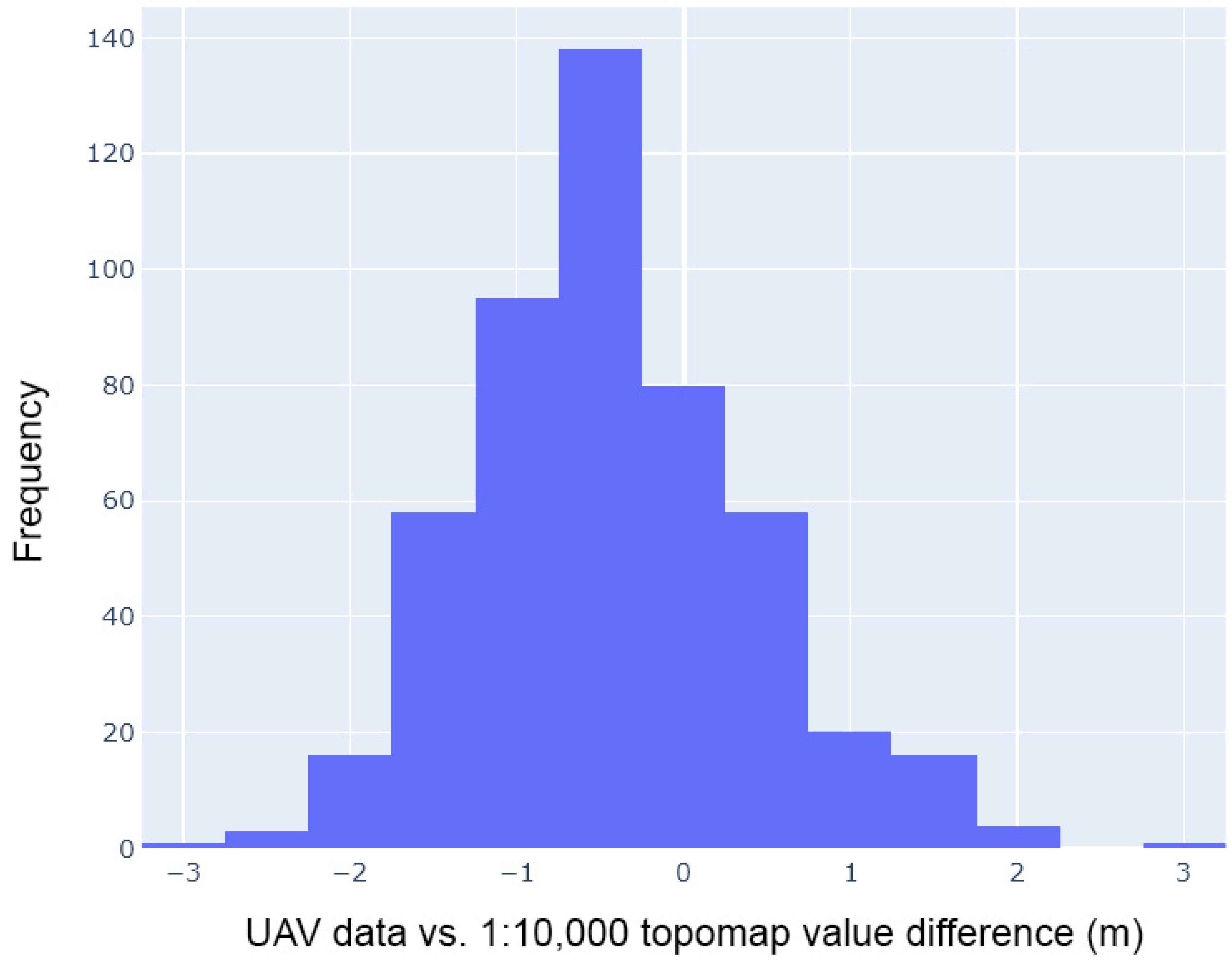
| Parameter | Value |
|---|---|
| Amount | 490 |
| Average | −0.422096 |
| Median | −0.483889 |
| St. deviation | 0.839484 |
| Minimum | −2.99682 |
| Maximum | 2.80948 |
| Q1 | −0.918266 |
| Q3 | 0.103119 |
Publisher’s Note: MDPI stays neutral with regard to jurisdictional claims in published maps and institutional affiliations. |
© 2021 by the author. Licensee MDPI, Basel, Switzerland. This article is an open access article distributed under the terms and conditions of the Creative Commons Attribution (CC BY) license (http://creativecommons.org/licenses/by/4.0/).
Share and Cite
Gafurov, A. The Methodological Aspects of Constructing a High-Resolution DEM of Large Territories Using Low-Cost UAVs on the Example of the Sarycum Aeolian Complex, Dagestan, Russia. Drones 2021, 5, 7. https://0-doi-org.brum.beds.ac.uk/10.3390/drones5010007
Gafurov A. The Methodological Aspects of Constructing a High-Resolution DEM of Large Territories Using Low-Cost UAVs on the Example of the Sarycum Aeolian Complex, Dagestan, Russia. Drones. 2021; 5(1):7. https://0-doi-org.brum.beds.ac.uk/10.3390/drones5010007
Chicago/Turabian StyleGafurov, Artur. 2021. "The Methodological Aspects of Constructing a High-Resolution DEM of Large Territories Using Low-Cost UAVs on the Example of the Sarycum Aeolian Complex, Dagestan, Russia" Drones 5, no. 1: 7. https://0-doi-org.brum.beds.ac.uk/10.3390/drones5010007