
Unmanned Autogyro for Mars Exploration: A Preliminary Study


Dipartimento di Scienze, Università degli Studi “Roma Tre”, Via della Vasca Navale n. 84, 00146 Rome, Italy
*
Author to whom correspondence should be addressed.
Drones 2021, 5(2), 53; https://0-doi-org.brum.beds.ac.uk/10.3390/drones5020053
Submission received: 28 April 2021
/
Revised: 8 June 2021
/
Accepted: 17 June 2021
/
Published: 18 June 2021
(This article belongs to the Special Issue Feature Papers of Drones)
Abstract
:Starting from the Martian environment, we examine all the necessary requirements for a UAV and outline the architecture of a gyroplane optimized for scientific research and support for (future) Mars explorers, highlighting its advantages and criticalities. After a careful trade-off between different vehicles suitable for a typical mission, some parameters are established to optimize the size and performance. In the second part, the project of the Spider gyroplane and the methodology used to balance the longitudinal masses are presented; in the third part, the parameters of the aerodynamic forces acting on the aircraft are highlighted to be able to focus them during the fluid dynamics simulations.
1. Introduction
“A journey of a thousand [miles] starts with a single step.”(Lao-Tsu)
Man has always turned his gaze to the sky: while the stars took the shape of the constellations and gave rise to myths, the planets soon became the abode of the gods. Their movement independent of the Earth’s rotation suggested a completely different nature than the stars: they were soon considered places such as our planet and, therefore, either inhabited or habitable.
The first successful landing on another planet was made by the Soviet Venera 7 probe on Venus on 15 December 1970, while Mars, after a partial landing of Mars 3, was conquered only in 1976 by two NASA Viking landers. Only recently, thanks to advances in technology, has it been possible to send the Ingenuity helicopter to wander around the Perseverance rover. Now the road to the Martian atmosphere is opened to UAVs: these vehicles allow a greater panoramic view than a rover while maintaining the possibility of examining, in detail and closely, details of Mars that could be of extreme scientific interest.
1.1. State of Exploration of Mars
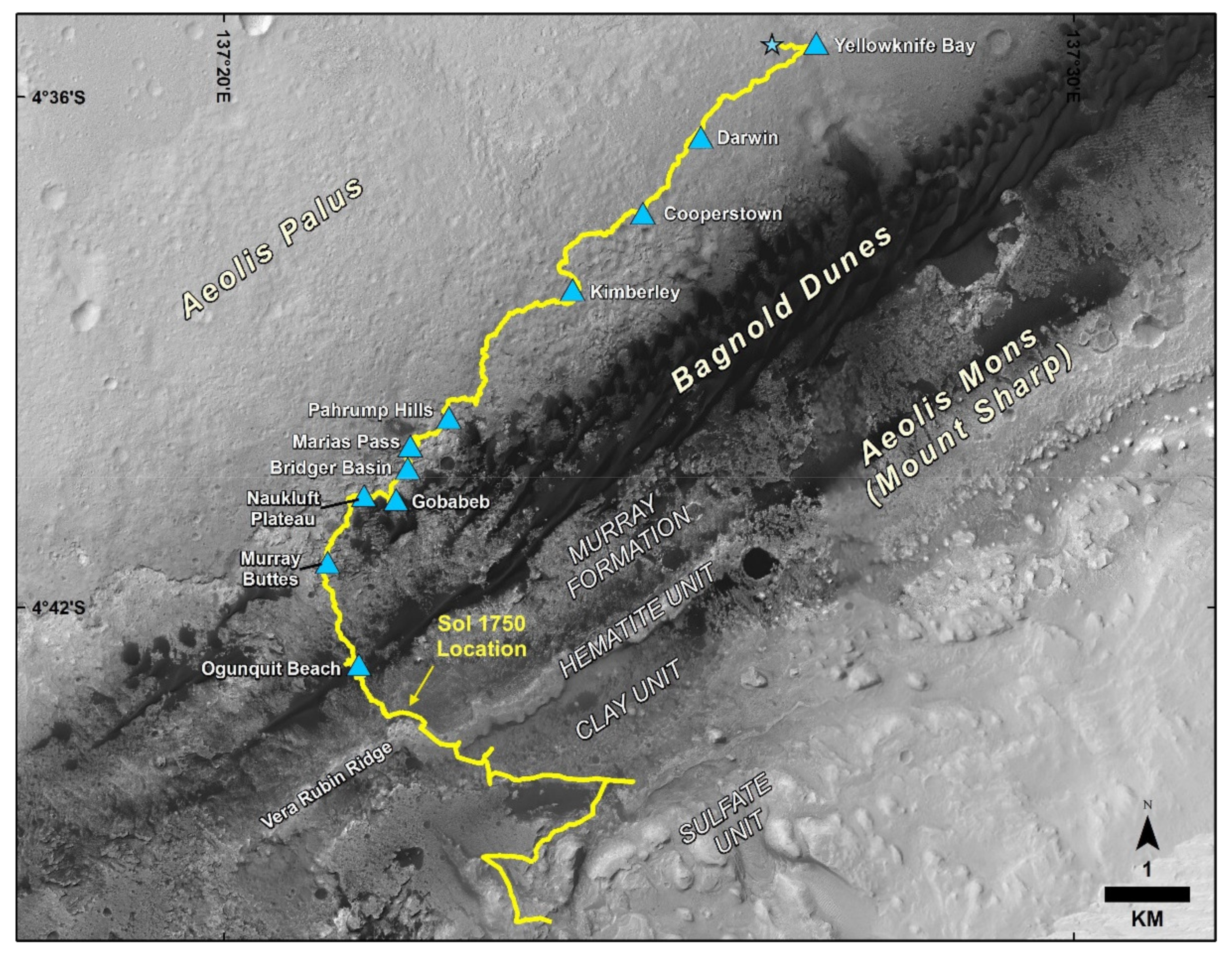
The exploration of planets is currently entrusted to probes and automatic machines that have the task of leading the way to human colonization. Automatic exploration systems have reached all the inner planets and several outer planets: in the last two decades, the attention has been focused on Mars. The continuous progress of aerospace and electronic technology has put the colonization of the “red planet” among the works of human ingenuity that can be completed in a few years and no longer a science fiction dream. Precursors of this last step are the probes and the rovers: multi-wheel robots that can make simple decisions and perform a series of tests: due to the harsh Martian soil, their movements are very cautious and, for some activities, dependent on the day-night cycle. In Figure 1, we can see the tortuous path taken by the Curiosity Mars rover: a journey of a few kilometers.
This type of vehicle is, therefore, very suitable for close-up exploration of the land, as it can capture every detail of the terrain but is unable to have a panoramic view of the landscape. On the other side, there are the observation satellites in Martian orbit: the Mars Reconnaissance Orbiter (with the HiRISE—High-Resolution Camera—onboard) is in orbit 450 km from the surface; although it is able to map the ground with great precision (HiRISE can produce images from which topography can be calculated to an accuracy of 0.25 m). It is absolutely evident there is a lack of a vehicle that is able to place itself reasonably far from the ground to be able to see a wider horizon but, at the same time, capable of grasping details and, if necessary, overlooking points that could be of extreme interest. Finally, the speed factor is important to quickly reach the points of greatest interest with respect to the point of arrival on the Planet.
1.2. Mission Concept
The operating conditions of a possible automatic flying vehicle (UAV: Unmanned Aerial Vehicle) on Mars are quite complex and, in some cases, they collide with each other. Mainly they are:
- The UAV must be rather simple and robust as it will first have to withstand the stresses due to launch, space flight, entry into the Martian atmosphere, and then, it will have to be deployed as more parts will surely have traveled folded.
- The vehicle must be extremely reliable as there is no maintenance required: many electronic systems and all critical mechanical systems must be redundant.
- The vehicle has a limited life span thus, it will be necessary to optimize his work to have specific and scheduled tasks.
- Its work is mainly carried out during the day, as it is equipped with solar cells to recharge the batteries. It is also equipped with multispectral sensors optimized for Martian light.
- The vehicle is meant to work with a rover, which, of course, will arrive at the same time. However, the two vehicles are not in symbiosis: the UAV will be able to fly away from the rover even for a considerable distance and for several days.
- Drones must, therefore, be able to store the large mass of scientific data it is intended to collect. Later, it will reach the rover and will download the data: it will then be the task of the land vehicle to act as a relay.
From these first considerations, it can be deduced that the vehicle must be a fair compromise between gross weight and payload.
1.3. Why an Autogyro?
An autogyro (from Greek αὐτός and γύρος, “self-turning”), also known as a gyroplane or gyrocopter, is a type of rotorcraft that uses an unpowered rotor in free autorotation to develop lift [1]. Forward thrust is provided independently, usually by an engine-driven propeller. While like a helicopter rotor in appearance, the autogyro’s rotor must have air flowing across the rotor disc to generate rotation and the air flows upwards through the rotor disc rather than down [2]. These types of flying machines were successful in the 1920s and 1930s when the performance of fixed-wing aircraft was far from flattering. Following the war events, it gave a strong impulse to the development of the helicopter, a vehicle that monopolized the technological development of the rotary wing [3].
Table 1 shows the comparison between the main flight characteristics of airplanes, helicopters, and autogyros: obviously, it should not be understood as a ranking in which we try to establish which is the “best flying machine,” but to stigmatize the different characteristics in order to find the most suitable for the needs of the mission [4].
The airplane is an excellent platform for instruments as it exhibits excellent stability (even in gusts of wind) and extreme maneuverability: unfortunately, it has a high stall speed due to its architecture. It would be possible to equip an aircraft with STOL (Short Take-Off and Landing) or VTOL (Vertical Take-Off and Landing) features at the price of a very high weighting of the structure, as they require the addition of “ad hoc” engines or aerodynamic surfaces [5].
The performance of the helicopter is very close to our desired in terms of stall speed: unfortunately, it turns out to be a very unstable platform and subject, as everyone knows, due to high vibrations. Furthermore, it is a mechanically very complex machine like its maneuvering [6].
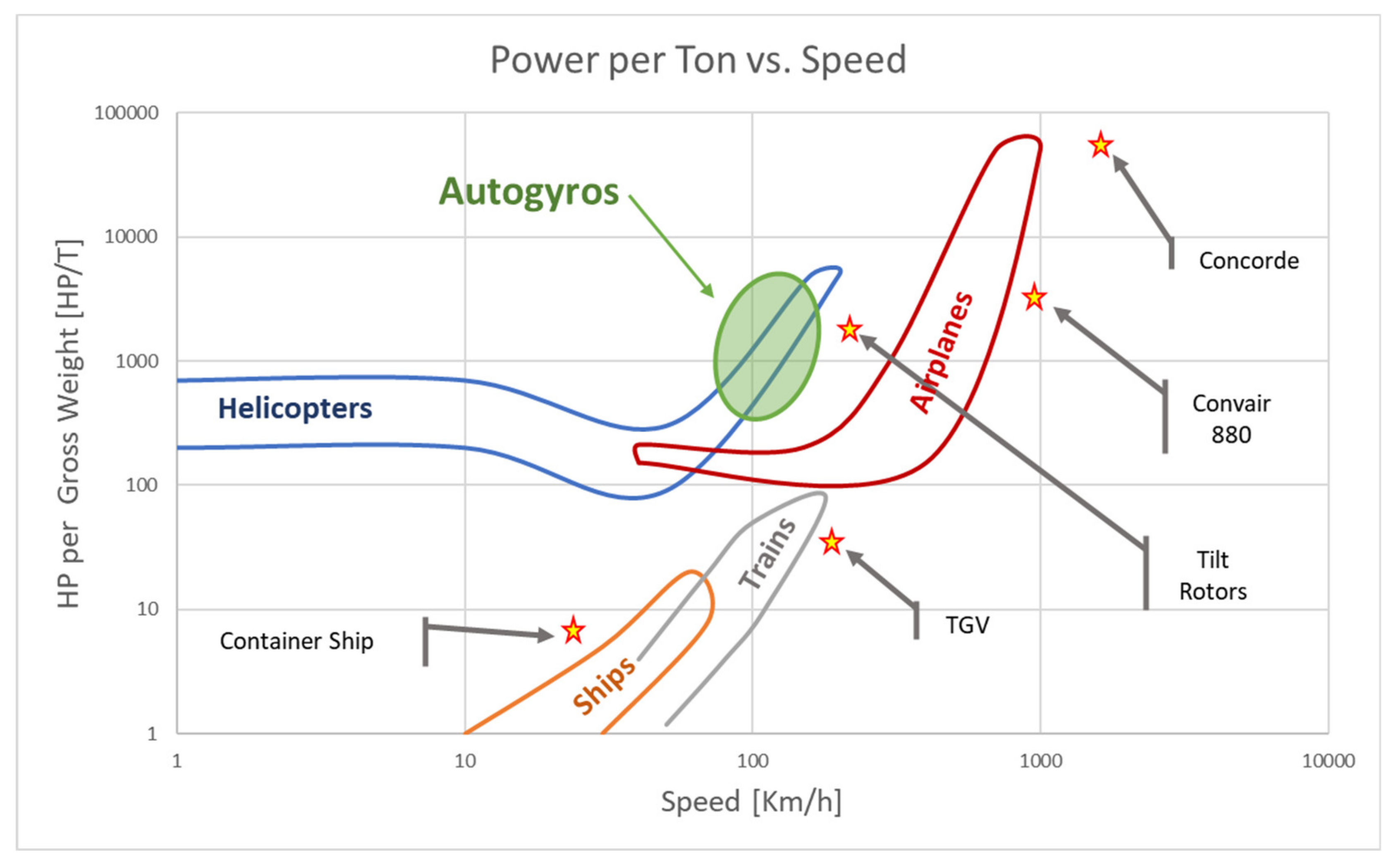
In Figure 2, we can see graphs showing horsepower per tons of gross weight versus speed for different families of transport or utility vehicles.
The behavior of ships and trains is immediately evident, which in the face of rather low power transport goods at a relatively low speed: even if it is not visible in the graph, all this is accomplished with a general economy of the service.
Helicopters, on the other hand, have a “useful speed” even zero as they are often called upon to perform missions such as “sky cranes”, that is to say, for lifting antennas or power lines above rivers, valleys, etc.
The gyroplanes (green zone) have been highlighted in the green zone.
2. Materials and Methods
2.1. The Environment: Mars
Mars is the planet that has always attracted the main scientific interest from the international community and the various space agencies, as demonstrated by the great commitment made in its study since the beginning of the exploration of the solar system. The planet has been studied for centuries, but only the beginning of the space age has allowed us to understand in detail many of its characteristics, until then only hypothesized. The space probes in orbit and the vehicles on the ground made it possible to collect a great variety of information, from the composition and internal structure to the interaction of the upper atmosphere with the solar wind (see Table 2).
The Atmosphere
The atmosphere has been the object of particular attention on our part because it is the gaseous medium through which our vehicle moves: since it is not equipped (because of the absence of oxygen in the Martian atmosphere) with an internal combustion engine but an electric one, we will only consider the aerodynamic and physics-chemical interactions with the gyro.
The Martian atmosphere (see Table 3) has a mass much less than that of the Earth: a reference value for the surface pressure can be considered 6.1 mbar, 3 orders of magnitude lower than the corresponding Earth value. This value is highly variable due to the great topographical differences of the surface. The temperature during the polar night can drop below the CO2 condensation point, resulting in the deposition of a relevant fraction of the atmospheric mass and the annual bimodal pressure cycle observed by landers and orbiters. The study on the isotopic and elementary ratios of atmospheric gaseous species [2] has shown that the primitive atmosphere of Mars, formed after the conclusion of the T-Tauri phase of the solar life cycle, was affected by a considerable process of gas removal due to different causes. The proposed values for the surface pressure primitive of Mars are all around 1 bar. The reduction of the atmospheric mass has mainly affected the currently predominant component that is carbon dioxide, primarily because of meteorite bombardment and atmospheric escape. Several authors have also highlighted the possible role played by the inclusion of carbon in carbonate minerals in a water-rich environment. Thus far, carbonates have not been detected on Mars in appreciable quantities, and, therefore, this effect, even if present, should be of secondary importance. In the atmosphere, both CO and O2 are observed, both derived from the dissociation of CO2.
The role of water on Mars has always been the subject of a large literature: in particular, H2O vapor exhibits highly variable atmospheric concentrations in space and time. The seasonal variations were observed in detail by the Mars Atmospheric Water Detector (MAWD) aboard the Viking 1 Orbiter and were confirmed by observations of the Thermal Emission Spectrometer (TES) instrument aboard the NASA MGS (Mars Global Surveyor) probe. Water vapor showed a maximum concentration during the waning phase of the northern hemisphere polar cap, when a fraction of the H2O, trapped as ice during the winter, sublimated into the atmosphere while a secondary maximum was present during the hemisphere spring. The surface plays a role both as a source and as a deposit for the water present in the atmosphere. The surface layers play an important role due to their hygroscopic character deriving both from the morphology (aggregates of mineral dust of various sizes, from centimeter to sub-millimeter) and from the mineralogical composition of the soils, on both seasonal and daily time scales. Several meters below the surface, some observational evidence of the MARSIS radar instrument (Mars Advanced Radar for Subsurface and Ionosphere Sounding) placed on board of the Mars Express probe, and observations of the Shallow Subsurface Radar (SHARAD), instrument onboard the Mars Reconnaissance Orbiter probe (MRO), suggested that there may be a large water reservoir, in the form of a permanent ice layer, probably a region rich in crystalline water dispersed in a matrix of mineral grains. To date, the presence of the underground water source has not yet been confirmed. Possible evidence in this sense was represented by the presence of “rampart” craters, peculiar Martian impact craters characterized by evidence of erosion by fluid agents, and by observations of the hydrogen concentration on Mars of the GRS experiment (Gamma Ray Spectrometer) on board of the Mars Odyssey probe.
In addition to gases and water ice clouds, the Martian atmosphere contains a considerable amount of mineral dust, the presence of which produces various observable phenomena. Among these, there were the dust devils, columns of dust with a diameter of the order of 10s of meters and over 6 kilometers in height that were raised from the surface by winds localized near the surface and dust storms, which can hide large areas surface to observations, for periods ranging from several days to covering the entire planet for several months, as observed during the summer of 2007 by instruments aboard the Mars Express and Mars Reconnaissance Orbiter missions.
2.2. Mars Environment: Pro and Cons
Although the Martian atmosphere, for density, gaseous composition, and solar radiation, does not allow human life if not adequately protected by pressure suits, the Navier-Stokes equations remain valid thus an aircraft can fly. Obviously, the diversity of the environment requires a profound redesign of the vehicle: this is to define unequivocally that, for example, a helicopter designed for the Earth will never be able to fly over Mars or vice versa [7,8,9,10,11]. The positive and negative factors of operating in the Martian atmosphere with a gyroplane will now be examined.
2.2.1. Pro and Cons
In this section, by examining the differences in the Martian environment, we see what the advantages and disadvantages of an air vehicle can be.
Cons
- The main problems for a flying vehicle in the Martian atmosphere derive from its very low density (about 1.7%), as the expression of lift is:
- Because the speed of sound is much lower (about 70% of that of the Earth), the tips of the blades approach the transonic regime much faster with the same rotor revolutions.
- Blades and wings operate in low Reynolds number flows: thus, they will need to be shorter and wider (thicker chord), but the profile drag is much higher.
In Equations (1)–(3) we see the expression of lift, in which:
is the lift of the vehicle, on Earth, on Mars.
is density of atmosphere, on Earth, on Mars.
is the speed of the vehicle.
In Equation (4), we have the comparison of the speed of sounds:
is the speed of sound on Earth, on Mars.
In Equation (5), we see the expression of the (Reynolds number) in which:
is the dynamic viscosity.
is the length of the chord of the wing profile.
In the face of the aforementioned strong difference in density, we do not have an equal lowering of the dynamic viscosity, thus that the operating conditions on Mars are found at low Reynold numbers.
Pros
- Gravity on Mars is just under a third of that on Earth.
- It is possible to build vehicles with a much lighter structure.
- The aerodynamic coefficient of drag is significantly lower.
2.2.2. The Tale of Two Planets
We can operate the first approach in general sizing by the similarity between the two planets since, regardless of the environment in which they operate, the balance laws of forces (and energies) must be the same.
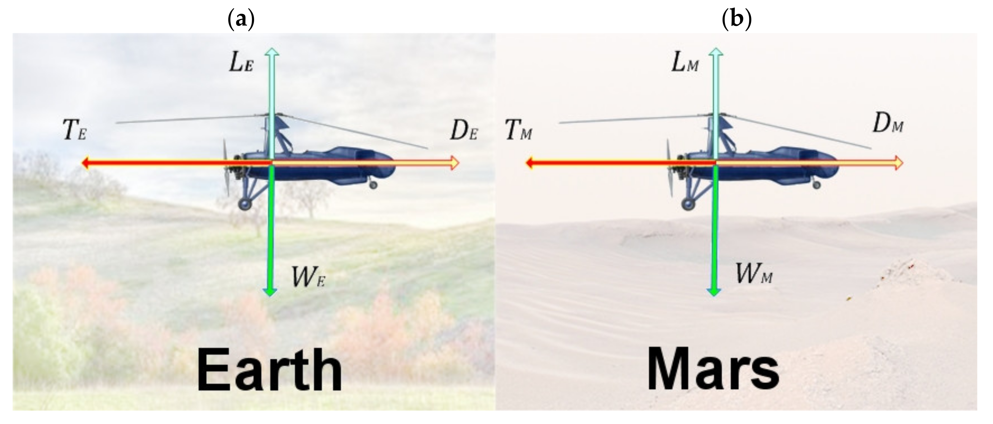
The balance of forces for the vehicle on Earth (moving at a constant speed and at a constant altitude) must be (see Figure 3a/left):
where:
- is the necessary thrust provided by the engine on Earth.
- is the drag of the vehicle in the Earth’s atmosphere.
- is the total lift of the vehicle in the Earth’s atmosphere.
- is the total weight of the vehicle on Earth.
Starting from the principle that thrust is only dependent on engine technology, we expand the other members, the drag is:
where:
- is the atmosphere density of Earth.
- is the velocity of the vehicle on Earth.
- is the coefficient of drag of the vehicle on Earth.
- is the lift surface of the vehicle.
For the lift, we have:
where:
- is the coefficient of lift of the vehicle on Earth.
For the weight, we have:
where:
- is the mass of the vehicle.
- is the surface acceleration of gravity on Earth.
The balance of forces for the vehicle on mars (moving at a constant speed and at a constant altitude) must be (see Figure 3b)
where:
- is the necessary thrust provided by the engine on Mars.
- is the drag of the vehicle in the Mars’ atmosphere.
- is the total lift of the vehicle in the Mars’ atmosphere.
- is the total weight of the vehicle on Mars.
Starting from the principle that thrust is only dependent on engine technology, we expand the other members, and the drag is:
where:
- is the density of Mars’ atmosphere.
- is the velocity of the vehicle on Mars.
- is the coefficient of drag of the vehicle on Mars.
- is the lift surface of the vehicle.
For the expression of the lift, we have:
where:
- is coefficient of lift of the vehicle on Mars.
For the weight, we have:
where:
- is the surface acceleration of gravity on Mars
Let us start working on the weight of the vehicle: with the same mass, we have that:
Then we have:
and
This means that all things being equal, the lower Martian gravity allows us to fly vehicles just under 3 times heavier (large): let us see how this affects the other parameters. For the necessary lift, we have:
hence:
Considering the density, we have:
Explicating with respect to the velocities:
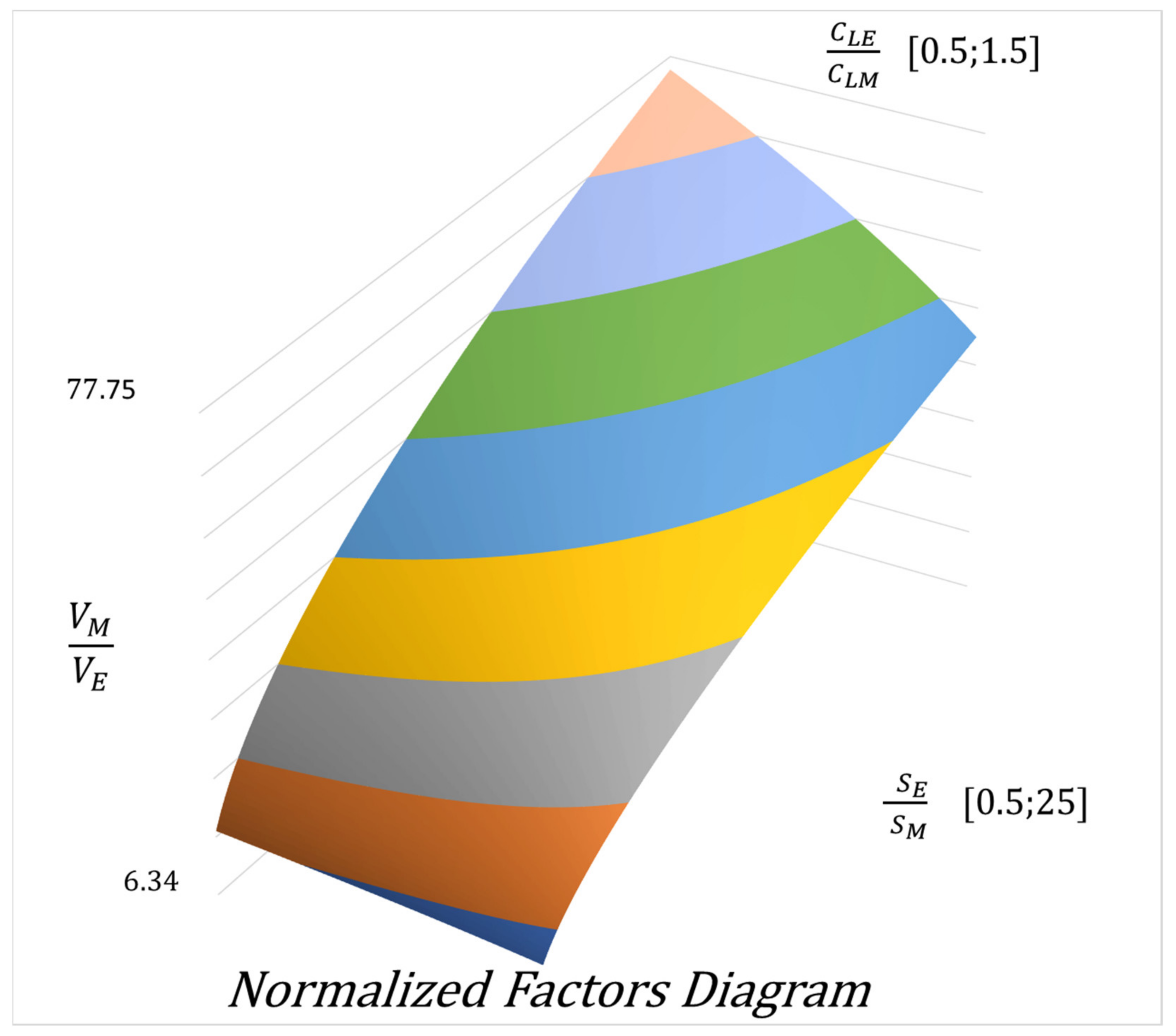
It is, therefore, possible to establish an optimal surface to evaluate the main parameters of a vehicle operating on Mars in an analog way with one optimized to operate on Earth.
The surface described by expression (22) is represented in Figure 4 below. The physical meaning was twofold: first of all, to design a vehicle that is optimized for the Martian environment, one must remain inside and on the borders of the surface described. Any departure from this will, therefore, lead to a penalty either in performance or otherwise such as for example in the ability to carry a heavy payload [12,13,14,15]. In other words, if you try to magnify a drone’s ability by moving away from the surface, this requires compensation thus, we can rightly consider it an excellent surface. The second meaning is the ability to be able to design a vehicle for Mars in analogy with a similar vehicle for Earth, i.e., the expression (22) is a sort of “transfer function” for the design between the two planets [16,17,18].
2.3. The Gyroplane
Based on all the considerations of the previous paragraphs, our working group has decided to develop a drone project for Martian exploration based on the architecture of the gyroplane since, according to the technologies present at state of the art, it is the one that satisfies all mission requirements.
2.3.1. The Mission: “Fly Like a Butterfly and Sting Like a Bee”
A gyroplane is not a hybrid; it is not a cross between various architectures: it is a vehicle with peculiar characteristics and capabilities that, in a Martian environment, are particularly highlighted. First of all, it is a much faster vehicle than a helicopter, which allows it, for the same amount of time, to explore a considerably greater area. Secondly, it can have a significantly heavier scientific payload for the same MTOW (Maximum Take-Off Weight). It is also less prone to gusts of wind, thus becoming a rather independent aerial platform with respect to the environment. It certainly does not have the vertical take-off and landing capacity of the helicopter, but this is compensated by extraordinarily strong STOVL (Short Take-Off and Vertical Landing) characteristics, being able to land and take off in just over 20 m. Certainly, the necessary spaces are widely available on Mars.
Since, as it is known, it was not possible to study a vehicle that can do everything at the same time, it was, therefore, necessary to define one or more missions in order to “tailor” the architecture and payload, and, therefore, we have predicted the following scenarios:
Pathfinder
In this first scenario. The vehicle proceeds as a forerunner of a possible land rover. Since the speed of the latter is very low and its proceeding on the Martian soil very cautious due to the impossibility of having a wide “observable horizon”, the aerial drone would be its “eye in the sky”. Therefore, its task should be mainly to find a safe and obstacle-free path for the Martian rover and, in the eventuality, to provide surveys and photographic evidence of interesting details of areas or rock formations that may be the subject of further study.
Precision Aerial Photogrammetry
The photographic mapping of Mars is mainly entrusted to satellite vehicles, which have already provided a good mapping of the planet but suffer from two major penalties: the lack of flexibility as the area framed in the FOV (field of view) is obviously linked to the trajectory orbital and the inability to further detail a particular area worthy of interest. All this, combined with the fact of not being able to have a resolution higher than a quarter of a meter, makes it the ideal means to create general maps but not detailed ones. Furthermore, it would be impossible to observe the same area through different hours of the day or the seventh, for example, the melting of an area of the ice cap: the two successive observations would be temporally spaced by two orbital passages. In this case, the gyroplane could overcome all these limitations.
Cargo Shuttle
Considering the ambitious human colonization project, a gyroplane is an ideal vehicle to support a human base on Mars. It can carry out SAR (Search And Rescue) missions of isolated astronauts, moving essential supplies (for example, batteries, oxygen, etc.) in a short time, or acting as an audio/video relay for telecommunications by starting to orbit in a circle at high altitude.
These are just a few scenarios in which a gyroplane can make a strong contribution.
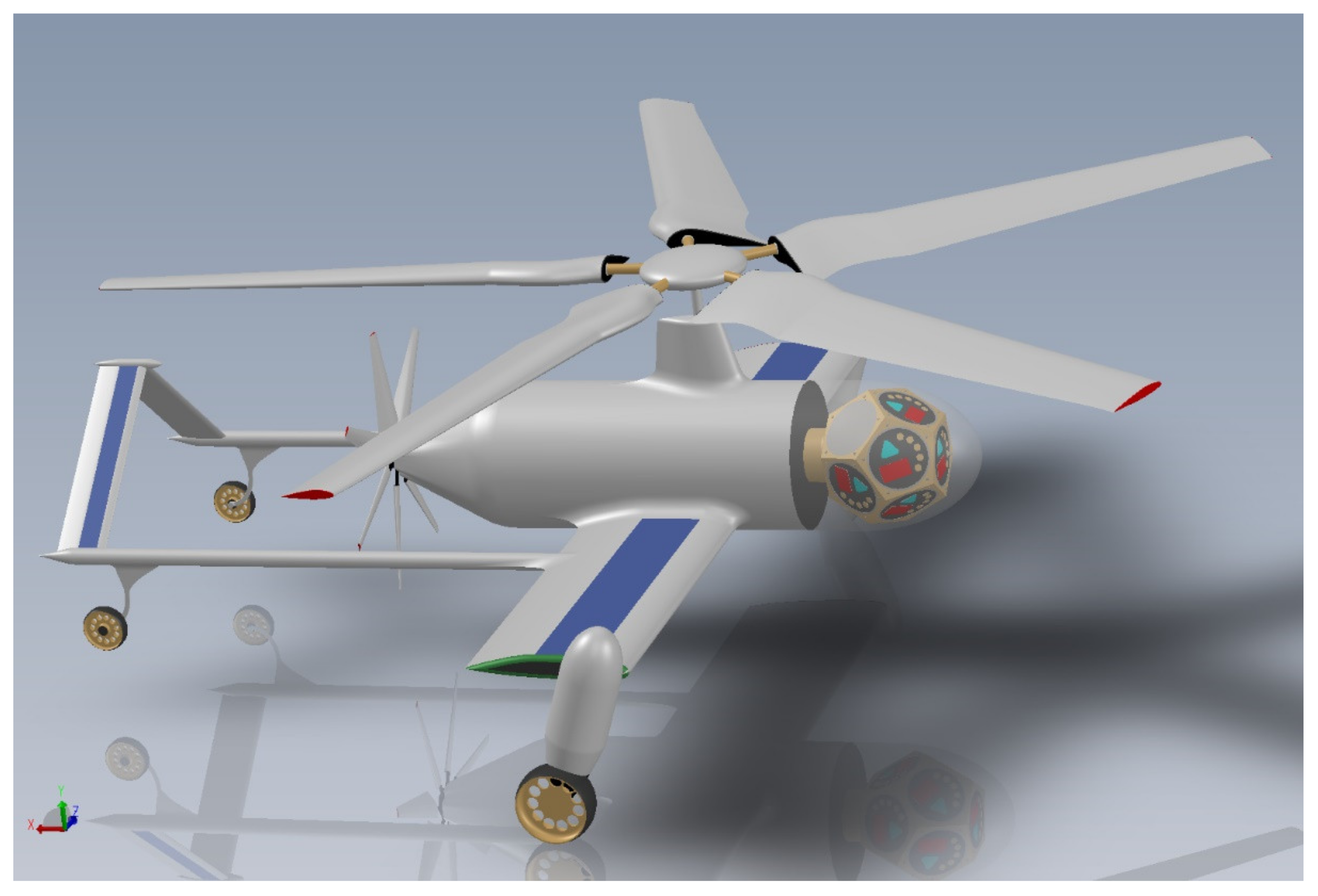
2.3.2. Spider
Our group has, therefore, given the name of Spider (see Figure 5) to the gyroplane for the evident similarities with the insect. The estimated characteristics of the vehicle are shown in Table 4 (see).
The gyroplane is composed of a few simple elements that almost all perform aerodynamic and structural functions (see Figure 6). The central body is composed of a carbon fiber cylinder, which contains the guidance and control systems, the OBC (On-Board Computer), which oversees all the autonomous piloting functions. The 2 wings are connected to the cylinder (cantilever); on their upper surface, there is a strip of solar cells, which has the task of recharging the batteries. At the end of each wing, there is a tip-tank that supports the main landing gear wheel: this has two positions retracted and deployed (see Figure 7). At about one-third of the wingspan, there are the 2 tail booms, which in turn support the V-shape tail wings; each of them has a strip of solar cells on the surface, which, like those of the wings, help recharge the batteries. Near the tail, there are also the 2 wheels of the rear landing gear. In the upper part, there is the “saddle” that supports the rotor, made up of 5 blades, each with double hinges (swing and flapping—not visible in the image). In the front, protected by a radome, there is an icosahedron with pentagonal faces: on each, there are a series of optical and electromagnetic sensors for exploration and navigation.
In the rear, conical part, there is the electric motor for the propeller (composed by seven blades) in a pushing configuration.
The choice of the particular type of fletching is due to the fact that the architecture allows them to be immersed in the direct flow of the propeller, thus that they are effective even at very low speed.
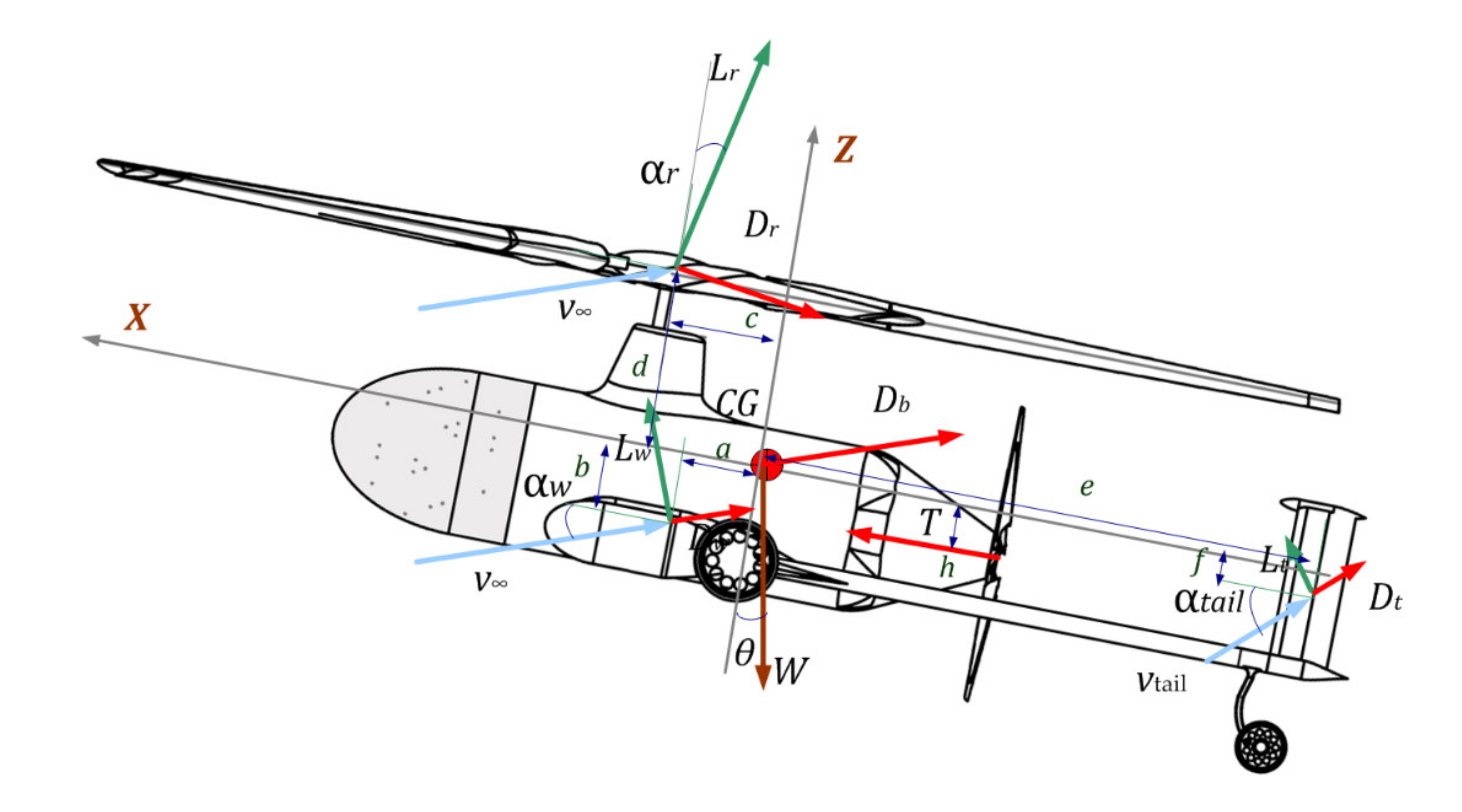
2.3.3. Longitudinal Balance
To correctly manage the positioning of vehicle systems and subsystems, it was necessary to accurately define the balance of forces and momentum in the vertical plane. Figure 8 (below) shows the forces acting on the vehicle in stationary conditions.
In this section, we considered the dynamic balance of forces on the vertical plane (X, Z) and momentum with respect to the Y-axis. In these conditions, the gyroplane proceeds at a constant speed. In the following discussion, the variation of density of the air with the variation of the altitude will not be considered, nor of the relative variation in propeller and rotor efficiency. We will consider these constant elements with reasonable approximation in a non-negligible altitude interval.
By definition:
Considering the X-axis:
where:
- is the lift force of the rotor.
- is the drag force of the rotor.
- is the lift of the wing.
- is the drag of the wing.
- is the lift of the tail.
- is the drag of the tail.
- is the angle between and the rotor plane.
- is the angle between and the wing.
- is the angle between (due to downwash) and the tail.
- is the angle of body axes and ground.
- is the weight of the vehicle.
- is the thrust.
For the balance of the forces on the Z-axis w have:
The balance around the Z-axis is:
Now considering a little , and , considering , h, f negligible for the expression (24)–(26) we have:
Thus the (23) becomes:
By grouping all the friction factors not dependent on the angles:
For the first member of (30), we have:
Posing:
For the second member of (30), we have:
Posing , for the third member of the (30), we have:
Explicating :
Taking into account dynamically the forces that contribute to the balance of forces, always remembering to check the positioning on the surface depicted in Figure 4, with the expressions (32), (34), and (35), we can move on to the physical sizing of the drone. Remember that a move away from the aforesaid surface entails a deviation from the optimal design conditions and that this is paid in terms of lowering the yield of some parameters.
2.3.4. Simulation
Now, it is necessary to analytically define the parameters to be searched for in the fluid dynamics simulation; for the lift of the wing, we have:
where:
- : mars atmosphere density
- : wing surface
- : relative speed (refer to air)
- : coefficient of lift of the wing
According to Taylor’s method, the last member can be separated in:
where:
- coefficient of lift at = 0
- : coefficient of lift at ≠ 0
Then, the expression (36) becomes:
Similarly, for the lift of the rotor we have:
where:
- : rotor disc surface
- : coefficient of lift at = 0
- : coefficient of lift at ≠ 0
For the lift of the tail, we have
where:
- : tailplane surface
- : the wing profile is symmetrical.
- : coefficient of lift at ≠ 0
The lift of the fuselage can be considered negligible () compared to the other forces involved.
For the drag of the wing, we have:
where:
- coefficient of drag at = 0
- : coefficient of drag at ≠ 0
Similarly, for the drag of the rotor we have:
where:
- coefficient of drag at = 0
- : coefficient of drag at ≠ 0
For the drag of the tail, we have:
where:
- coefficient of drag at = 0
- : coefficient of drag at ≠ 0
For the drag of the body, we have:
where:
- : exposed surface of the body
- coefficient of drag at = 0
- : coefficient of drag at ≠ 0
By grouping the expressions (38), (39), (40), (41), (42), (43) and (44) in matrix form, we can write:
where for we have the following diagonal matrix:
We evaluated the vehicle’s coefficients of by inserting the CAD model (developed with SolidWorks®) into its fluid dynamics application (see Figure 9), testing several angles of attack in order to define all the parameters of the matrix and thus be able to obtain a dynamic model of our vehicle.
3. Conclusions
The exploration of Mars by means of aerial drones is an opportunity that is opening with the Ingenuity helicopter: everything suggests that it will be followed by many others. In our work, we first wanted to reiterate the state of the art of planetary exploration, which, at the moment, is focused on rovers, highlighting their criticalities and limitations by briefly examining the Curiosity Mars Rover case study. Next, we examine all the constraints that a flying vehicle mission imposes in the Martian atmosphere, finding all the functional requirements that cannot be absent.
From a trade-off with other flying vehicles, we arrive at the result that an autogyro proves to be the most suitable for that role, both for the payload and for the reasonable shortness of take-off and landing spaces.
From the examination of the Martian environment, several problems have been highlighted, such as low density, the need to operate at low Reynolds numbers, and the fact that in those conditions, the speed of sound is rather low enough to operate even at low rpm the extremity of the blades are nearly in the transonic zone. On the other hand, gravity is much lower, and this allows for much heavier payloads with the same performance.
From the operational similarity between two flying vehicles on Mars and on Earth, we come to define an “optimal surface” that identifies the limitations and characteristics of the operating conditions of an aerial drone.
In the second part, we illustrated our study for a gyroplane: we defined a series of missions such as pathfinder, precision aerial photogrammetry, and cargo shuttle, which, now, seem to be the most useful ones to be entrusted to an autonomous vehicle. We presented our “spider” vehicle and defined the longitudinal balance, as this type of aircraft is particularly sensitive to the position of the center of gravity; therefore, consequently, its positioning affects the internal arrangement of the avionics, services and all the necessary equipment, as well as the payload. In the last part, we defined, which are the aerodynamic parameters necessary to fully define a simulation. This work is only a preliminary part of a larger study for the design of a Martian flying vehicle.
Author Contributions
Conceptualization, E.P. and F.L.; methodology, E.P.; validation, F.L.; formal analysis, E.P.; investigation, F.L.; resources, F.L.; data curation, E.P.; writing—original draft preparation, E.P.; writing—review and editing, F.L.; supervision, F.L.; funding acquisition, F.L. All authors have read and agreed to the published version of the manuscript.
Funding
This research received no external funding.
Institutional Review Board Statement
Not applicable.
Informed Consent Statement
Not applicable.
Data Availability Statement
Not applicable.
Conflicts of Interest
The authors declare no conflict of interest.
Abbreviations
Symbols and Coefficients.
| Lift | |
| Air Density Mars | |
| Air Density Earth | |
| Coefficient of Lift | |
| Drag | |
| Coefficient of Drag | |
| Thrust | |
| Surface (aerodynamic) | |
| Angle of Attack (local) | |
| acceleration of gravity on Mars | |
| acceleration of gravity on Earth | |
| Mass of the vehicle | |
| angle between ground | |
| Weight | |
| Weight on Mars | |
| Weight on Earth |
References
- Capon, P.T. Cierva’s First Autogiros. Aeropl. Mon. 1979, 7, 234–240. [Google Scholar]
- NASA. Planetary Fact Sheet—Metric. Available online: https://nssdc.gsfc.nasa.gov/planetary/factsheet/ (accessed on 1 March 2021).
- Thomson, D.G.; Houston, S. The Aerodynamics of Gyroplanes; University of Glasgow: Glasgow, UK, 2010. [Google Scholar] [CrossRef]
- Glauert, H. A General Theory of the Autogyro. In Aeronautical Research Committee Reports and Memoranda No. 1111; Cranfield University: Cranfield, UK, 1926. [Google Scholar]
- Wheatley, J.B. An Aerodynamic Analysis of the Autogyro Rotor with a Comparison between Calculated and Experimental Results; NACA: Moffett Field, CA, USA, 1934; Volume 487. [Google Scholar]
- Wheatley, J.B. An Analytical and Experimental Study of the Effect of Periodic Blade Twist on the Thrust, Torque and Flapping Motion of an Autogyro Rotor; US Government Printing Office: Washington, DC, USA, 1937; p. 591.
- Houston, S.S. Validation of a rotorcraft mathematical model for autogyro simulation. J. Aircr. 2000, 37, 403–409. [Google Scholar] [CrossRef]
- Singh, J.; Dadhich, A. Optimization of Autogyro for Preliminary Development of Personal Flying Vehicle. Int. J. Innov. Res. Sci. Eng. Technol. 2017, 6. [Google Scholar]
- Wu, W. A Controller for Tracking Steep Glide Slopes for an Unmanned Gyroplane. Br. J. Appl. Sci. Technol. 2015, 10, 1–11. [Google Scholar] [CrossRef]
- Leishman, J.G. Development of The Autogyro: A Technical Perspective. J. Aircr. 2004, 41, 765–781. [Google Scholar] [CrossRef]
- Petritoli, E.; Leccese, F. Unmanned Autogyro for Advanced SAR Tasks: A Preliminary Assessment. In Proceedings of the 2020 IEEE 7th International Workshop on Metrology for AeroSpace (MetroAeroSpace), Pisa, Italy, 22–24 June 2020; pp. 615–619. [Google Scholar] [CrossRef]
- Vainilavičius, D.; Augutis, V.; Malcius, M.; Bezaras, A. Analysis of autogyro rotor balancing and vibration. In Proceedings of the 2015 IEEE Metrology for Aerospace (MetroAeroSpace), Benevento, Italy, 4–5 June 2015; pp. 416–420. [Google Scholar] [CrossRef]
- Wang, R.; Wu, L.; Bing, F. Automatic Landing Control Design of Gyroplane. In Proceedings of the 2019 IEEE 3rd Advanced Information Management, Communicates, Electronic and Automation Control Conference (IMCEC), Chongqing, China, 11–13 October 2019; pp. 1480–1484. [Google Scholar] [CrossRef]
- Young, L.A.; Aiken, E.; Lee, P.; Briggs, G. Mars rotorcraft: Possibilities, limitations, and implications for human/robotic exploration. In Proceedings of the 2005 IEEE Aerospace Conference, Big Sky, MT, USA, 5–12 March 2005; pp. 300–318. [Google Scholar] [CrossRef] [Green Version]
- Young, L.A.; Aiken, E.W.; Gulick, V.; Mancinelli, R.; Briggs, G.A. Rotorcraft as Mars Scouts. In Proceedings of the IEEE Aerospace Conference, Big Sky, MT, USA, 9–16 March 2002; Volume 1, pp. 1–378. [Google Scholar] [CrossRef] [Green Version]
- Pergola, P.; Cipolla, V. Mission architecture for Mars exploration based on small satellites and planetary drones. Int. J. Intell. Unmanned Syst. 2016. [Google Scholar] [CrossRef]
- Braun, R.D.; Wright, H.S.; Croom, M.A.; Levine, J.S.; Spencer, D.A. Design of the ARES Mars airplane and mission architecture. J. Spacecr. Rocket. 2006, 43, 1026–1034. [Google Scholar] [CrossRef]
- Serna, J.G.; Vanegas, F.; Gonzalez, F.; Flannery, D. A review of current approaches for UAV autonomous mission planning for Mars biosignatures detection. In Proceedings of the 2020 IEEE Aerospace Conference, Big Sky, MT, USA, 7–14 March 2020; pp. 1–15. [Google Scholar]
Figure 1.
This map shows the route driven by NASA’s Curiosity Mars rover, from the location where it landed in August 2012 to its location in July 2017 (Sol 1750), and its planned path to additional geological layers of lower Mount Sharp (image and caption: © NASA).
Figure 1.
This map shows the route driven by NASA’s Curiosity Mars rover, from the location where it landed in August 2012 to its location in July 2017 (Sol 1750), and its planned path to additional geological layers of lower Mount Sharp (image and caption: © NASA).

Figure 2.
Most common vehicles: power per ton vs. speed.

Figure 3.
The balance of forces for the vehicle on Earth (a/left) and on Mars (b/right).

Figure 4.
Normalized surface of the factors in expression (22).

Figure 5.
Spider Gyroplane: a prospective view.

Figure 6.
Four views of the drone.

Figure 7.
Main landing gear and tip tanks: deployed (a/left) and retracted (b/right).

Figure 8.
The balance of forces and momentum.

Figure 9.
Two images taken from a more extensive simulation of the behavior of the Spider drone in the Martian atmosphere ( = 10 m/s). On the right, the pressure gradient on the vehicle surface, while on the left the flow lines in the same conditions.
Figure 9.
Two images taken from a more extensive simulation of the behavior of the Spider drone in the Martian atmosphere ( = 10 m/s). On the right, the pressure gradient on the vehicle surface, while on the left the flow lines in the same conditions.


Table 1.
Comparison of the main flight characteristics of airplanes, helicopters, and autogyros.
| Characteristic | Type of Vehicle | ||
|---|---|---|---|
| Airplane | Helicopter | Autogyro | |
| Stability | Good | Poor | Particularly good, even at low speeds |
| VTOL | Possible but limited | Engine-powered main rotor | Yes: Pre-rotators |
| Hovering | Not Possible | Possible | Extremely low flight speed, almost hovering a |
| Stall | Stalls: recovery maneuver required | Stalls: autorotation maneuver required | Impossible: full controllable even at even in the absence of thrust |
| Maneuvering | Easy | Complex | Easy |
a Horizontal speed not negligible but extremely low.
Table 2.
Mars/Earth Comparison 1.
| Parameter | Mars | Earth | Ratio Mars/Earth |
|---|---|---|---|
| Mass (1024 kg) | 0.64171 | 59.724 | 0.107 |
| Equatorial radius (km) | 3396.2 | 6378.1 | 0.532 |
| Polar radius (km) | 3376.2 | 6356.8 | 0.531 |
| Surface gravity (m/s2) | 3.71 | 9.80 | 0.379 |
| Surface Atmosphere density (kg/m3) | 0.020 | 1.2210 | 0.01638 |
| Surface Speed of Sound (m/s) | 240 | 340 | 0.705 |
| Solar irradiance (W/m2) | 586.2 | 1361.0 | 0.431 |
| Number of natural satellites | 2 | 1 |
1 Source National Space Science Data Center (NSSDC).
Table 3.
Martian Atmosphere 1.
| Parameter | Value | Notes |
|---|---|---|
| Surface pressure: | 6.36 mb | @ mean radius: variable from 4.0 to 8.7 mb depending on the season |
| Surface density | 0.020 kg/m3 | |
| Scale height | 11.1 km | |
| Total mass of the atmosphere | 2.5 × 10¹⁶ kg | |
| Average temperature | 210 K (−63 °C) | |
| Diurnal temperature range | 184 K to 242 K (−89 to −31 °C) | |
| Wind speeds | 2–7 m/s (summer) 5–10 m/s (fall) 17–30 m/s (dust storm) | |
| Atmospheric composition (by volume) | Carbon Dioxide (CO2)—95.1% Nitrogen (N2)—2.59% Argon (Ar)—1.94% Oxygen (O2)—0.16% Carbon Monoxide (CO)—0.06% | Major (%) |
| Water (H2O)—210 Nitrogen Oxide (NO)—100 Neon (Ne)—2.5 Hydrogen-Deuterium-Oxygen (HDO)—0.85 Krypton (Kr)—0.3 Xenon (Xe)—0.08 | Minor (ppm) |
1 Source: National Space Science Data Center (NSSDC).
Table 4.
Spider: characteristics and performances (estimated).
| Max Takeoff Weight | Main Rotor Diameter | Length 1 | Wingspan | Cruise Speed | Range 2 | Endurance 2 |
|---|---|---|---|---|---|---|
| 10 | 2.25 | 1.75 | 1.85 | 45 | ~10 | 1.5 |
| kg | m | m | m | km/h | km | h |
1 Without rotor. 2 At cruise speed.
Publisher’s Note: MDPI stays neutral with regard to jurisdictional claims in published maps and institutional affiliations. |
© 2021 by the authors. Licensee MDPI, Basel, Switzerland. This article is an open access article distributed under the terms and conditions of the Creative Commons Attribution (CC BY) license (https://creativecommons.org/licenses/by/4.0/).
Share and Cite
MDPI and ACS Style
Petritoli, E.; Leccese, F. Unmanned Autogyro for Mars Exploration: A Preliminary Study. Drones 2021, 5, 53. https://0-doi-org.brum.beds.ac.uk/10.3390/drones5020053
AMA Style
Petritoli E, Leccese F. Unmanned Autogyro for Mars Exploration: A Preliminary Study. Drones. 2021; 5(2):53. https://0-doi-org.brum.beds.ac.uk/10.3390/drones5020053
Chicago/Turabian StylePetritoli, Enrico, and Fabio Leccese. 2021. "Unmanned Autogyro for Mars Exploration: A Preliminary Study" Drones 5, no. 2: 53. https://0-doi-org.brum.beds.ac.uk/10.3390/drones5020053