
Acoustic-Based UAV Detection Using Late Fusion of Deep Neural Networks


Department of Aeronautical and Automotive Engineering, Loughborough University, Loughborough LE11 3TU, UK
*
Author to whom correspondence should be addressed.
Drones 2021, 5(3), 54; https://0-doi-org.brum.beds.ac.uk/10.3390/drones5030054
Submission received: 19 May 2021
/
Revised: 23 June 2021
/
Accepted: 23 June 2021
/
Published: 26 June 2021
(This article belongs to the Special Issue Advances in Deep Learning for Drones and Its Applications)
Abstract
:Multirotor UAVs have become ubiquitous in commercial and public use. As they become more affordable and more available, the associated security risks further increase, especially in relation to airspace breaches and the danger of drone-to-aircraft collisions. Thus, robust systems must be set in place to detect and deal with hostile drones. This paper investigates the use of deep learning methods to detect UAVs using acoustic signals. Deep neural network models are trained with mel-spectrograms as inputs. In this case, Convolutional Neural Networks (CNNs) are shown to be the better performing network, compared with Recurrent Neural Networks (RNNs) and Convolutional Recurrent Neural Networks (CRNNs). Furthermore, late fusion methods have been evaluated using an ensemble of deep neural networks, where the weighted soft voting mechanism has achieved the highest average accuracy of 94.7%, which has outperformed the solo models. In future work, the developed late fusion technique could be utilized with radar and visual methods to further improve the UAV detection performance.
1. Introduction
Multirotor Unmanned Aerial Vehicles (UAVs) are a type of UAV propelled by more than one rotor. In this paper, the terms UAV and drone will be used interchangeably to refer to multirotor UAVs. While UAVs’ initial use was limited to the military sector [1], private owners and companies are presently utilizing them in a growing number of applications such as art, cinematography, documentary productions and deliveries. Additionally, governments are increasing drone use for public health and safety purposes, such as supporting firefighters, ambulance services and search-and-rescue operations [2]. The lists continue to expand as UAV technology advances, improving their performance while reducing their price. However, this widespread use of drones has drawn significant attention to the security risks, especially those associated with airspace breaches and drone-to-aircraft collisions.
In 2018, researchers at the University of Dayton Research Institute studied the effect of a drone striking a plane’s wing during flight. They discovered that the UAV could fully penetrate the wing’s leading edge and could cause catastrophic damage at higher speeds [3]. Germany has warned of a recent increase in drone interference, after reporting 92 drone-related incidents in their airspace during 2020, with one third of the cases resulting in air traffic being severely disrupted [4]. Even with reduced air traffic due to the pandemic, drone related disruptions continue to rise. Unwelcome UAV activity has proven to be severely costly and dangerous, and methods for their identification must be implemented and improved.
Hostile drone intrusions need to be detected as early as possible to ensure that countermeasures can be taken to neutralize them. The four detection methods currently in use are visual-, radar-, radio- and acoustic-based. With UAVs getting smaller and camouflaging more with the surrounding environment (for example: DJI Mini 2 [5]), cameras can sometimes fail to identify their presence [6]. Radars also struggle to reflect signals from small targets, and autonomous drones can bypass radio detection [7]. Thus, this project focuses on the acoustic detection of multirotor UAVs, through the use of deep learning methods, which can then be used together with the other detection techniques to improve the rate of success in UAV identification.
Standard classification models through supervised learning have been established by published research studying audio signals [6,8,9,10,11,12]. In this paper, the supervised learning methodology focuses on the binary classification of UAV and background. Any mix of sounds comprising drones is labelled as UAV, while all the other sounds are labelled as background.
Most published research on acoustic drone identification has used raw audio formatted in mono-channel, with a 16-bit resolution and a sampling frequency of 44.1 kHz [1,13,14]. There are a multitude of different pre-processing and feature extraction parameters to choose from, such as which time-frequency features to extract, what audio clip length to use, or if there should be overlap between clips [15,16,17]. Hence, a sensitivity study is needed to obtain the optimum pre-processing and feature extraction parameters for acoustic UAV detection. Additionally, there is a lack of publicly available datasets of drones in different real-world environments. To counteract this, some studies have artificially augmented the collected drone audio clips with other environmental sounds [1,15,16].
Features from the raw audio are extracted for model training with the aim to reduce the dimensionality of the data, disregarding redundant information and simplifying the training task [12]. For traditional machine learning, an extensive list of features must be manually extracted and optimized to fine-tune the algorithm. If such features are not optimal for the classification objective (e.g., drone detection), the performance of the model will be limited. Hence, extracting features becomes an additional challenge, as there is no guarantee that they are optimized for the classification objective [18]. Feature extraction is less of a problem when working with deep learning models, which perform best with features closer to the original audio signals, such as mel-spectrograms [19]. The neural network layers can then extract important information from the more general features, training themselves for the objective [20].
The state-of-the-art deep learning architectures used in audio classification models include Convolutional Neural Networks (CNNs), Recurrent Neural Networks (RNNs) and Convolutional Recurrent Neural Networks (CRNNs) [14,15,16,21]. CRNNs are an early fusion of the two networks, where the RNN processes the output of the CNN [19]. Eklund [12] states that the classification task and the type of data fed to the model may drive the decision on which model architectures to use. In general, RNNs perform better in natural language processing applications, whereas CNNs are best suited for image processing tasks. This is because RNNs contain the memory elements for context on the previous inputs of the time series [22], while CNNs possess the filtering property of the visual system for processing images [23]. Since the features extracted from raw audios are stored in a graphic format, CNNs should outperform RNNs, as confirmed by Al-Emadi et al. [15]. Despite Jeon et al. [16] concluding the opposite, possibly due to a difference in the construction of the models and their layers, both papers have confirmed the validity of utilizing deep learning for acoustic drone detection.
This report aims to investigate which model architecture (CNN, CRNN or RNN) shows the highest performance for the acoustic identification of UAVs, and then to introduce a form of late fusion of a network ensemble for acoustically detecting drones. Inspired by the conventional ensemble methods, such as random forest and AdaBoost [24], it is believed that an ensemble of classification models would perform better than the solo models. To the best of the authors knowledge, hard voting and weighted soft voting methods have not been tested for the acoustic identification of drones, although similar forms of late fusion networks have given promising results for other audio classification problems [21,25]. Therefore, the main contributions of this paper are as follows:
- Reinforce the viability of utilizing deep neural networks for the detection of multirotor UAVs with acoustic signals;
- Investigate which model architecture (CNN, CRNN, or RNN) performs the best for acoustic UAV identification;
- Evaluate the performance of late fusion networks compared with solo models and determine the most suitable voting mechanism in this study.
The remainder of this article is structured as follows: Section 2 discusses the methodology used for this project, detailing the data preparation, model training setup and model constructions. Section 3 provides and discusses the experimental results, comparing the performance of all the created models and detailing how the findings compare to previous research. Section 4 summarizes the conclusions and recommends future work.
2. Methodology
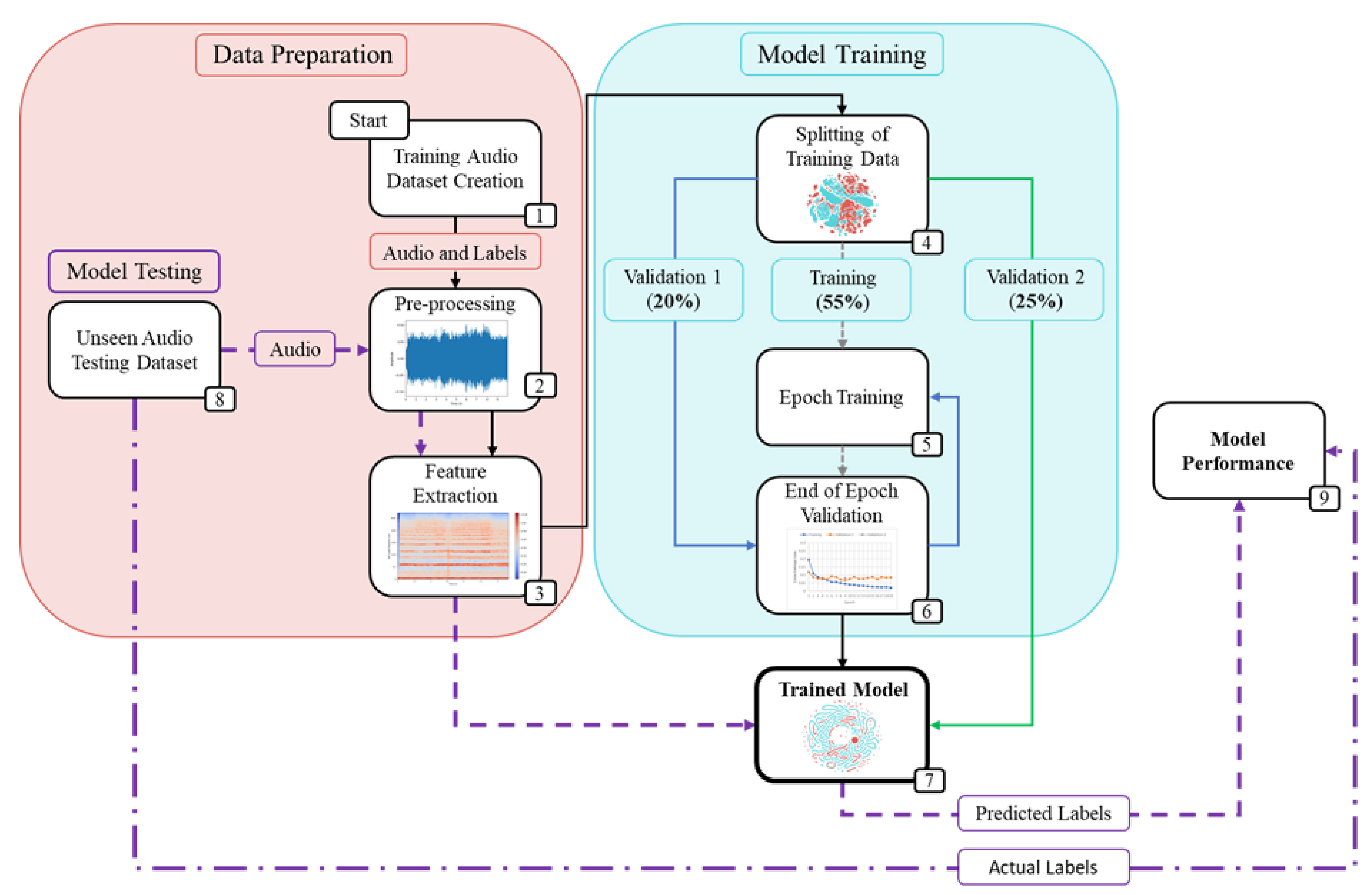
The workflow diagram, as shown in Figure 1, illustrates the structure and methodology used in this study.
Python 3.8 was the programming language used for this project, and the packages utilized include scikit-learn 0.23.2 [26], TensorFlow 2.4.1 [27] and librosa 0.8.0 [28]. Scikit-learn was used for the preparation of the training data for model training, splitting the dataset into training and validation subsets. TensorFlow was used to build and train the deep neural networks. Librosa was used for the feature extraction from raw audio to mel-spectrograms.
2.1. Data Preparation
All collected audio files were reformatted to mono-channel, with a 16-bit resolution and a sampling frequency of 44.1 kHz. Table 1 provides a complete breakdown of the composition and size of each dataset used in this study. Information for recreating these acoustic datasets can be found in the Data Availability Statement.
2.1.1. Training Audio Dataset
The training dataset used for this project was composed of different multirotor UAVs and background audios taken from online sources. The drones used to generate the UAV dataset are DJI Inspire 1, Mavic Air 2, Phantom 2, 3 and 4 Pro, the Parrot Bebop and Mambo, plus a range of other custom-built multirotor UAV sounds. These different drone audios were chosen because they can help the deep neural networks to train on the more general features of UAVs. The aim was to prevent the model from overfitting to more specific features (such as the specific frequency of a blade spinning in one particular drone model) and, hence, struggle to detect the drones it has not been trained on.
The positive training dataset contains drone audio artificially mixed with background audio, by adding the two signals together, enabling the model to deal with drones in real-world environments.
The sounds of a hypothetical airport environment were used to create the background training audios, because this is where the proposed model would operate. The most dangerous zones for drone strikes are beyond airport limits, in the take-off and landing zones. The location imagined for this project was an airport located near to a beach and some roads, in a tropical environment, to train and test the models on a variety of different sounds. The background sounds (Background-1, 2, 3 and 4) include planes, helicopters, traffic, thunderstorms, wind and quiet settings. Background-3 also includes 330 s of helicopter audio collected outside with an iPhone 12 Mini.
2.1.2. Unseen Audio Testing Datasets
To adequately evaluate the performance and generalization of a model, it is necessary to use a dataset that contains audio that the model has never been trained on. In this study this dataset is referred to as an unseen augmented testing dataset, and it is made up of a positive set (UAV) and a negative set (no UAV, or background). The positive dataset was composed of the audio from two drones (DJI Mini 2 and RED5 Eagle), recorded in a quiet room that was not included in the training dataset. These audios were augmented with new background sounds taken from online sources. To mimic the drone at differing distances from the microphone, compared to the background audios, three levels of difficulty were used in the testing dataset, where the decibel levels of the mixed audios were increased or reduced accordingly. Follow the link in the Data Availability Statement for more information on the testing data.
The negative unseen dataset is composed of the same background audios used for the positive dataset, in addition to extra audio from each background scene to equalize the number of positive and negative testing data (see Table 1). The audios were split up into 1 s lengths, with each second used as a test sample.
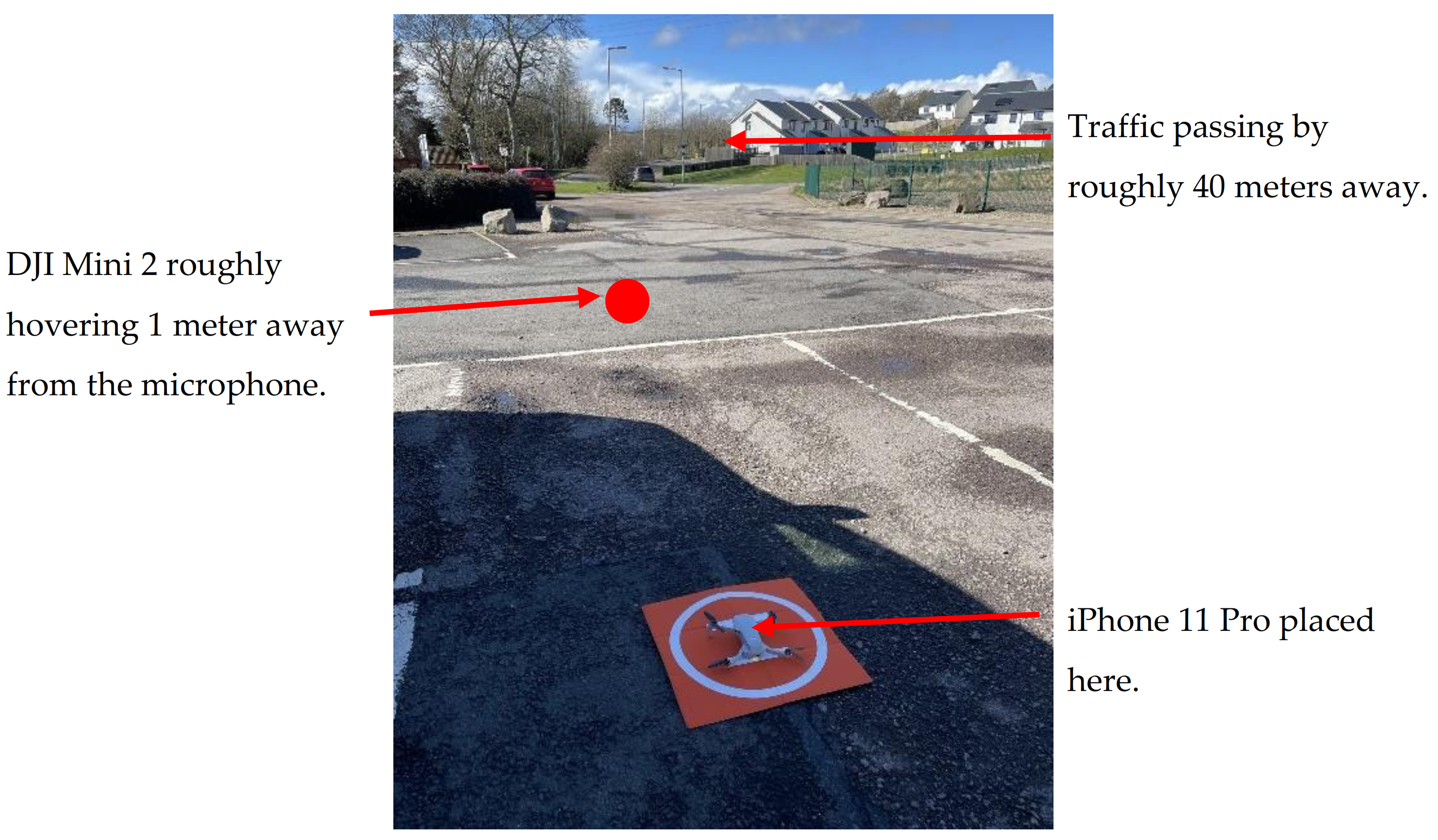
A small real world testing set was also created to verify that the model is functional in real environments (corresponding to Section 3.4). For the positive testing set, 213 s of audio from a DJI Mini 2 hovering near a road were collected (Figure 2), plus 60 s with a helicopter flying above. The negative testing set contains 273 s of the sounds near the same road, without the drone.
2.1.3. Audio Pre-Processing and Feature Extraction
Although the sampling rate of the raw audio is 44.1 kHz, the code for extracting the features was set at 22.05 kHz to reduce the required data storage by half and avoid the model training becoming significantly and unnecessarily more computationally demanding. Preliminary tests showed no noticeable benefit in using a higher sampling rate, which was to be expected, since the typical frequency range of a UAV lies under 1.5 kHz [29]. Additionally, Al-Emadi et al. [15] achieved high performance scores using a lower sampling rate (16 kHz).
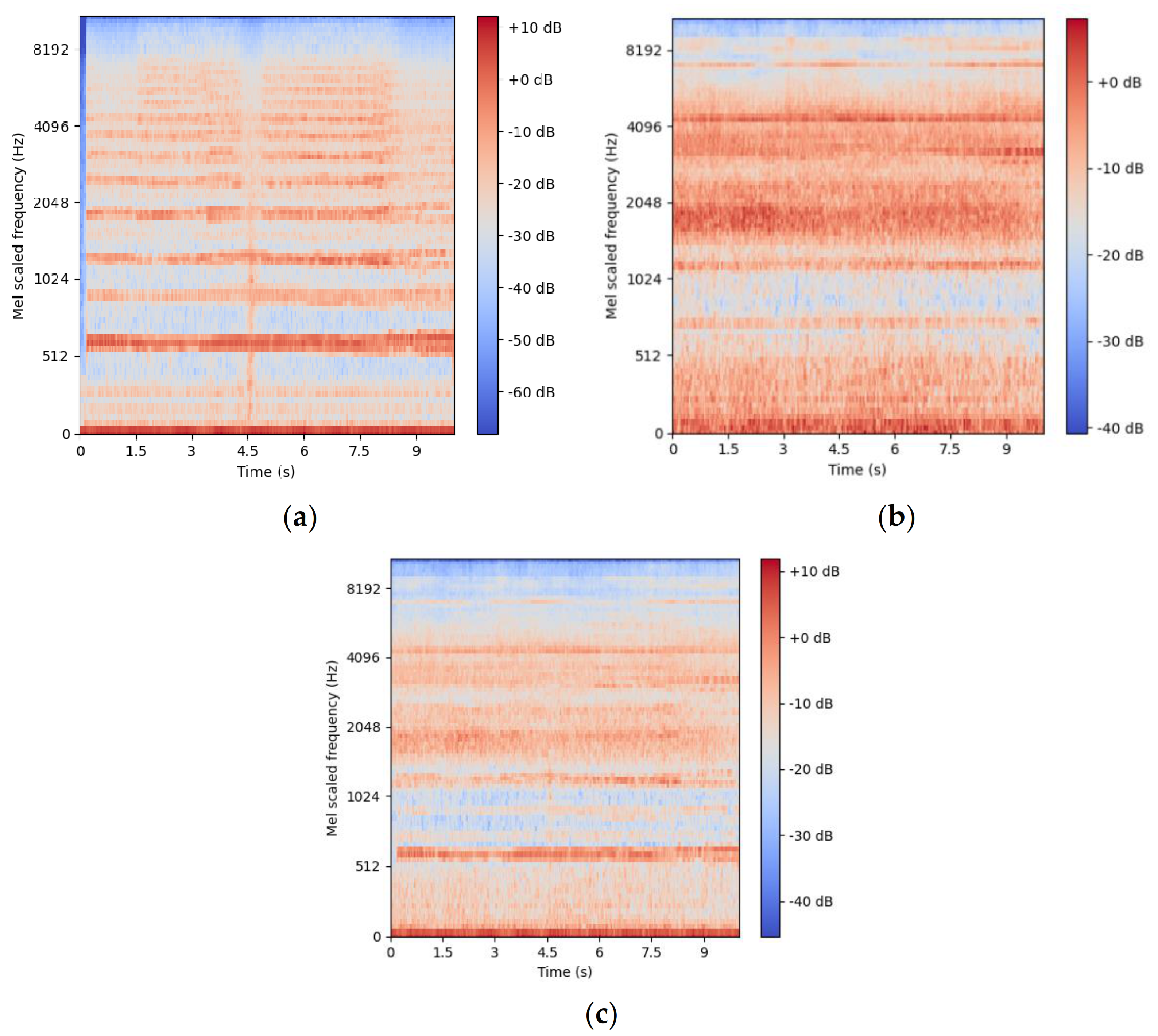
Through a sensitivity study, the optimal pre-processing parameters and features to extract (for model training of acoustic UAV detection) were determined empirically as 1 s segments of mel-spectrogram features, with 90 mel-frequency bins and no overlapping segments. The number of FFT for the mel-spectrogram extractions is 2048. Figure 3 shows the features extracted from the raw audio and fed to the deep learning models using these optimal extraction parameters, illustrating the differences between the mel-spectrograms of a UAV (Figure 3a), the background (Figure 3b) and the artificial mixing of the two (Figure 3c).
2.2. Model Training
The training dataset needed to be split into three subsets (training, validation 1 and validation 2), before model training could commence. The split used for this project was 55% training, 20% validation 1 and 25% validation 2 (Figure 1), which is similar to that which Sigtia et al. used [30].
For training, a learning rate of 0.0001 was used [31] with the TensorFlow Keras optimizer, Adam. A small batch size of 16 was applied, because of previous published work showing that small batch sizes of 32 or less can achieve the best training stability and generalization performance [32]. This was also confirmed by preliminary experiments for this project, where different batch sizes were tested, and the best results were obtained with 16. The cross-entropy loss (also referred to as loss here) is calculated using TensorFlow [33]. An increase in loss would indicate a divergence in the predicted probability from the actual label.
Early stopping and model checkpoints were utilized to save the best model during training, and to limit the chance of the model overfitting to the training dataset. The validation 1 cross-entropy loss was used to adjust network weights and to monitor model training (Figure 1).
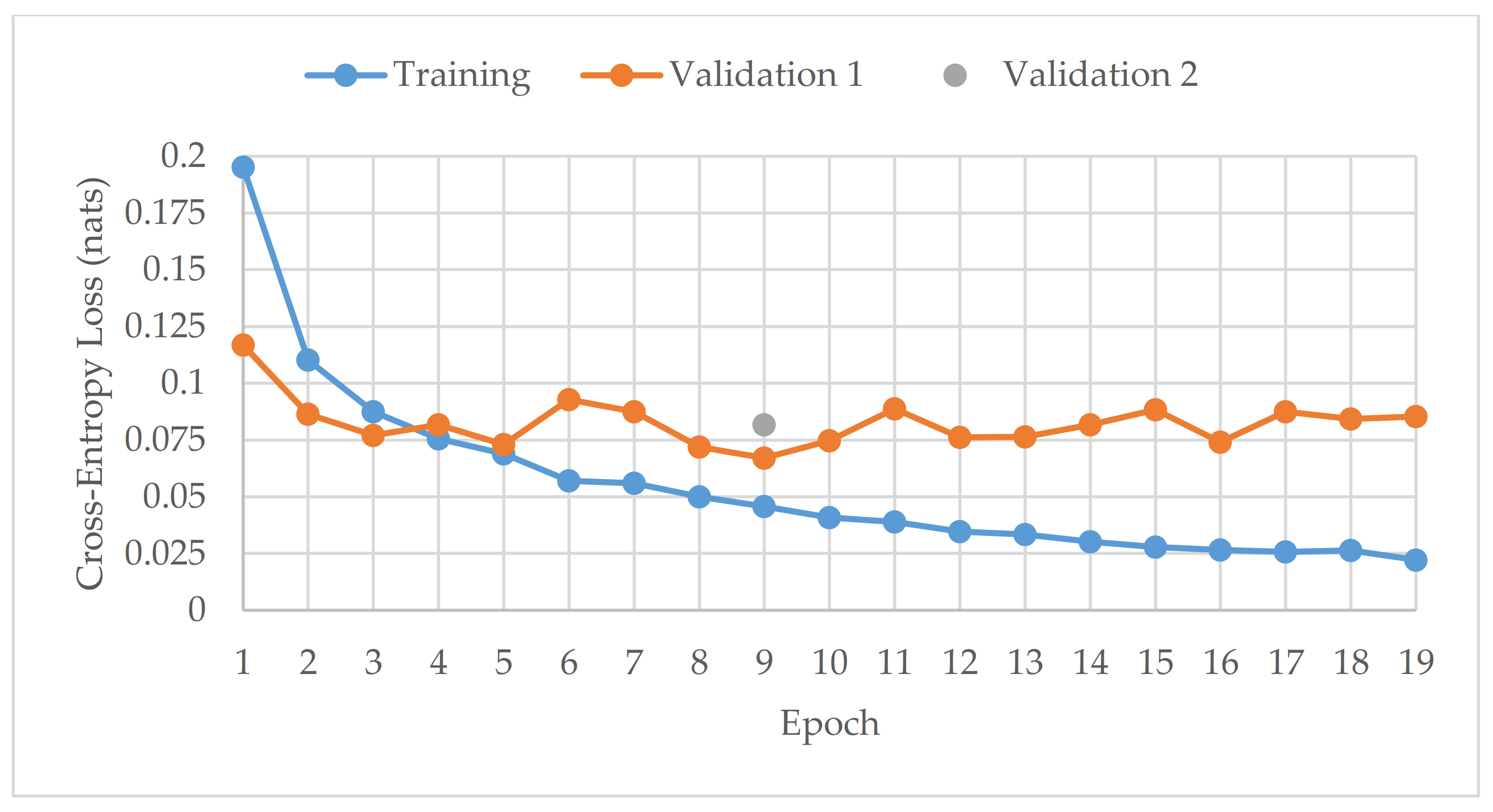
Training aimed to minimize the loss by adjusting the model weights at the end of each epoch, and the epoch model with the lowest validation 1 loss score was saved. If there was no further reduction in the cross-entropy loss value after 10 consecutive epochs, training stopped [15,16]. This is demonstrated by Figure 4, which shows the cross-entropy loss during the training history of the CNN model reported in Table 2.
In Figure 4, the minimum validation 1 loss occurred at epoch 9; training stopped at epoch 19 and the validation 2 subset was tested on the epoch 9 model. The benefit of implementing model checkpoints is shown by the increasing divergence between the validation 1 loss and the training loss curves after epoch 9 (Figure 4). With the validation 1 loss no longer improving, the model started to overfit to the training data, as shown by the continuously decreasing training loss curve. The low loss results obtained from the validation 2 subset gives substantial premise that the model has not overfit; however, it is not enough to ensure that the classification model would perform as intended with new audios.
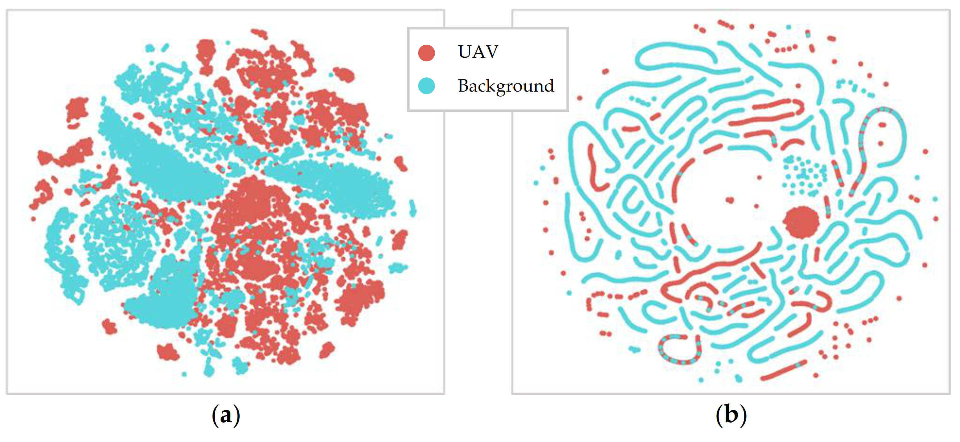
Figure 5 illustrates what reorganization the training dataset undergoes through model training for deep learning, by using t-SNE graphs. With t-SNE, the high-dimensional features shown in Figure 4 can be visualized more simply on a two-dimensional map. Figure 5a is a t-SNE visualization of the training dataset input, while Figure 5b is a visualization of the training output when the trained model optimizes the location of the training data’s features to improve classification performance. Figure 5b shows significantly more defined separation between UAV and background datapoints, compared to Figure 5a, with some small errors indicated by the proximity of some blue and red points.
2.3. Optimised Solo Models
Table 2, Table 3 and Table 4 summarize the different model architectures used and their hyperparameters. When constructing the CNN and CRNN models, a similar number of parameters was aimed for to ensure that the parameter size would not be the reason for a difference in performance between the two models. CNNs have convolutional layers to perform the filtering operation, while RNNs have Long-Short Term Memory (LSTM) layers to take into consideration the memory elements of previous observations.
The RNN top performing model presented by Jeon et al. [16] was recreated, and its performance compared with the models created for this study (Table 2 and Table 3). Table 4 shows the architecture of the RNN model, with some adaptation to complete the model architecture, as highlighted in grey. The dropout rate was 0.5, the learning rate was set to 0.0005 using the Adam optimizer, the batch size to 64 and the model training was stopped if the validation 1 loss did not reduce over 3 epochs of training [16] (only for the RNN model). These parameters differ from the CNN and CRNN models’ because the RNN model is entirely based on Jeon et al. [16], which includes using the same early stopping and batch sizes, whereas the parameters used for the CNN and CRNN models were found empirically and from the findings of past papers [32]. The recreated RNN model was then trained on the same training dataset as all the other models.
2.4. Late Fusion Networks
To the best of the authors knowledge, a late fusion of networks had not been tested to see if model performance can further improve for acoustic UAV identification. In this study, a standard hard voting and a weighted soft voting system were integrated, and their results compared.
The tested voting ensemble were made up of ten models (either all CNNs or CRNNs) with marginally differing hyperparameters. The ideal benefit of the late fusion networks tested is that less hyperparameter optimization work should be necessary, since ten different models would be working collectively. To conclude if this assumption is true, the hyperparameters used in the late fusion networks were set arbitrarily. Therefore, if the performance of the late fusion network is better than the optimized solo models, it shows that less effort will be required for the specific classification problem.
2.4.1. Hard Voting Setup
In the hard voting setup, the ten trained models vote either 1 for UAV or 0 for background, and their values are summed. If the overall value is 0–4, the hard voting model outputs a 0 (background) and, if the value is 5–10, it outputs a 1 (UAV). The decision of including 5 as a UAV prediction is because it is better to have more false positives than false negative results, since the purpose of this classification model is to detect hostile drones.
2.4.2. Weighted Soft Voting Setup
The weighted soft voting model goes one step further, considering the more ambiguous results. Instead of outputting a 0 or a 1, each of the ten solo models outputs a certainty value between 0 and 1 (known as a soft value). The closer the value is to 1, the more certain the model is that the audio contains a UAV. When the value is close to 0.5, the model is uncertain about any prediction it outputs. The soft voting system allows models with higher probability values to have more weight in the final result. For example, if one model has a probability value of 0.40, another of 0.45 and a third of 0.99, the respective hard voting output would be 0, 0 and 1. The hard voting model would therefore output 0 as its prediction. However, the soft voting model would give a higher weight to the probability value of 0.99, resulting in an output of 1.
The soft voting model also has a weighted component that considers how well each solo model had performed against the validation 2 subset at the end of training, by using the validation 2 accuracy results. The individual model’s accuracy is subtracted by the average value of all models, resi. The weight of the soft voting of this model is then wi = resi + 1/n, where n is the number of models. In this way, it satisfies that the summation of the weights equals 1.
2.5. Model Evaluation
Once the solo models and late fusion networks were constructed, training and performance evaluations were conducted to find the top performing models. Each model was trained on the training dataset and then tested on the unseen augmented audio dataset ten times to account for the effect of the random training components, enable the evaluation of the model stability and allow a fair comparison among the models. The performance of the models is evaluated using the metrics, accuracy and F-score, described by the following Equations (1) and (2), where TP represents the true positives, TN the true negatives, FP the false positives and FN the false negatives:
3. Results
All the results are illustrated on box and whisker plots that include ten independent runs for each model. For the calculation of the interquartile range, the exclusive method has been used.
3.1. Solo Model Performance Evaluation on the Unseen Augmented Dataset
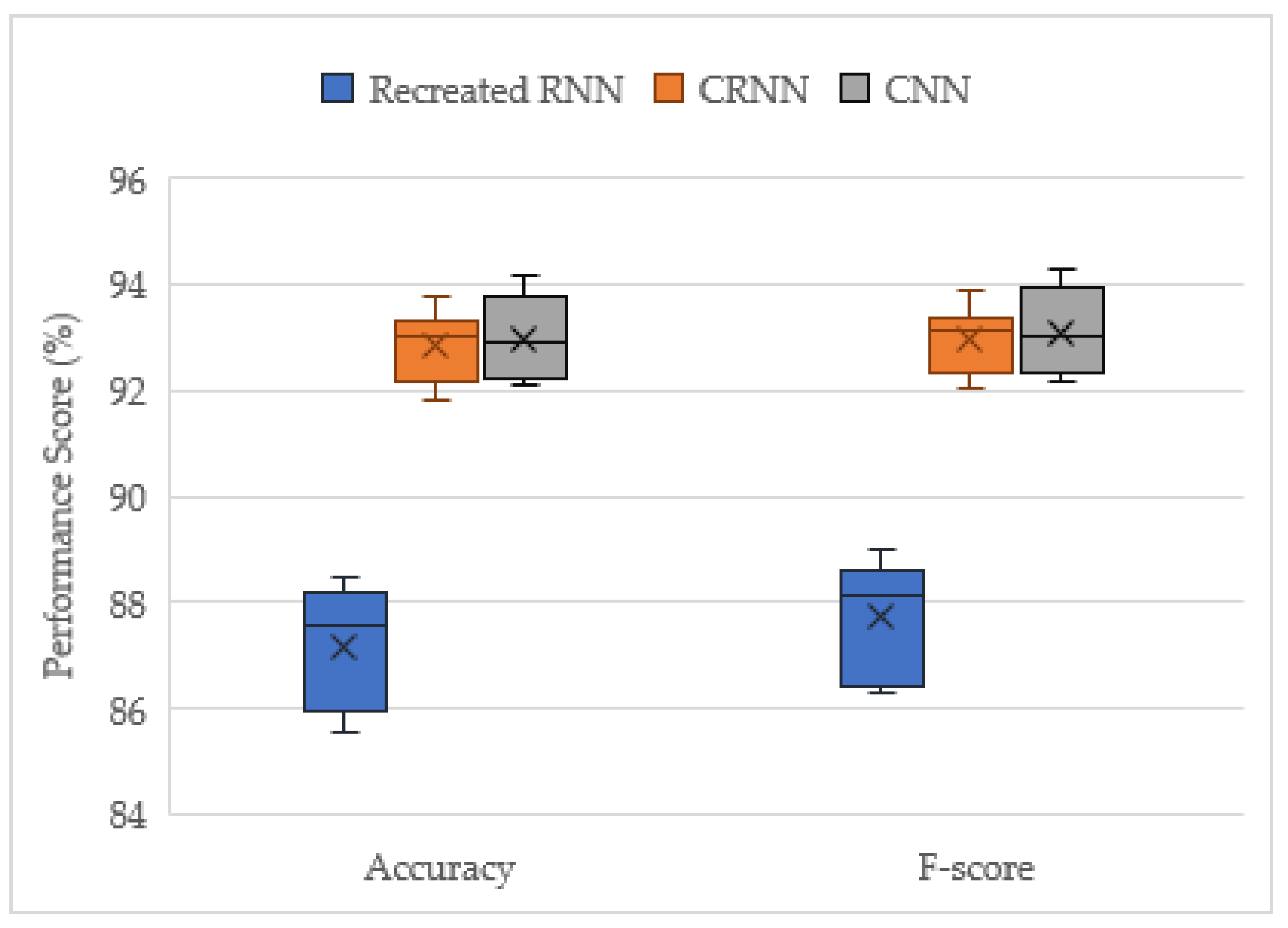
The solo models’ evaluation scores are shown in Figure 6. The CRNN and CNN models were found to be the best suited for the acoustic identification of UAVs, in agreement with previous findings [15], and with the fact that CNN models are the best performers with image processing tasks, since the features extracted from the raw audio are stored in a graphic format [12]. The recreated RNN model performed significantly worse, which was to be expected from a theoretical standpoint, since RNNs are more successful in natural language processing rather than image processing applications [12].
The performance difference between the CNN and the CRNN models is negligible, with both models achieving similar mean and median scores for accuracy and F-score, with slightly higher top performance scores for CNN, as illustrated by the larger interquartile range (Figure 6). This means that there is no significant benefit in using the CRNN or RNN models for acoustic UAV identification. The only potential benefit with the CRNN model would be that it has a more stable performance [15], as shown by the smaller interquartile range in Figure 6. For this project, late fusion was utilized on both the CRNN and CNN models to verify if the voting of models improves classification performance and to determine which model performs best in a voting ensemble.
3.2. Late Fusion Networks’ Performance Evaluation on the Unseen Augmented Dataset
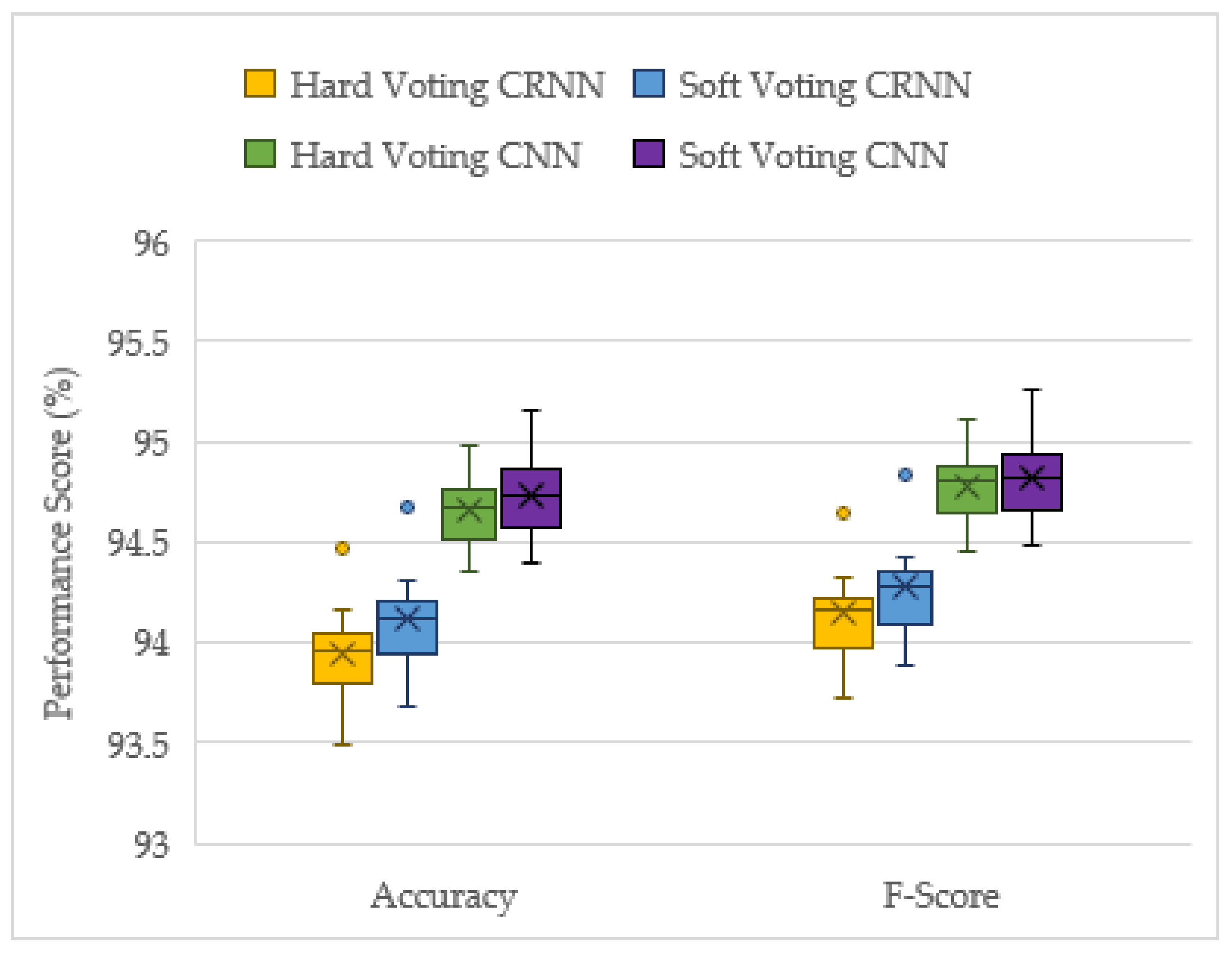
The late fusion models were trained and tested ten times and their results are compared in the box and whisker plot of Figure 7. The results conclude that the CNN voting ensemble outperforms the CRNN one. Additionally, the weighted soft voting CNN model shows a moderately higher overall performance compared to the hard voting CNNs, and this is also the case for the CRNN voting models. Therefore, it can be concluded that weighted soft voting outperforms hard voting, and that the weighted soft voting CNN model is the best performer of the four ensemble models. This confirms that CNNs are the best suited models for this feature processing task [12] and CRNN models have no added benefit for acoustic UAV identification in this case.
3.3. All Models Performance Comparison
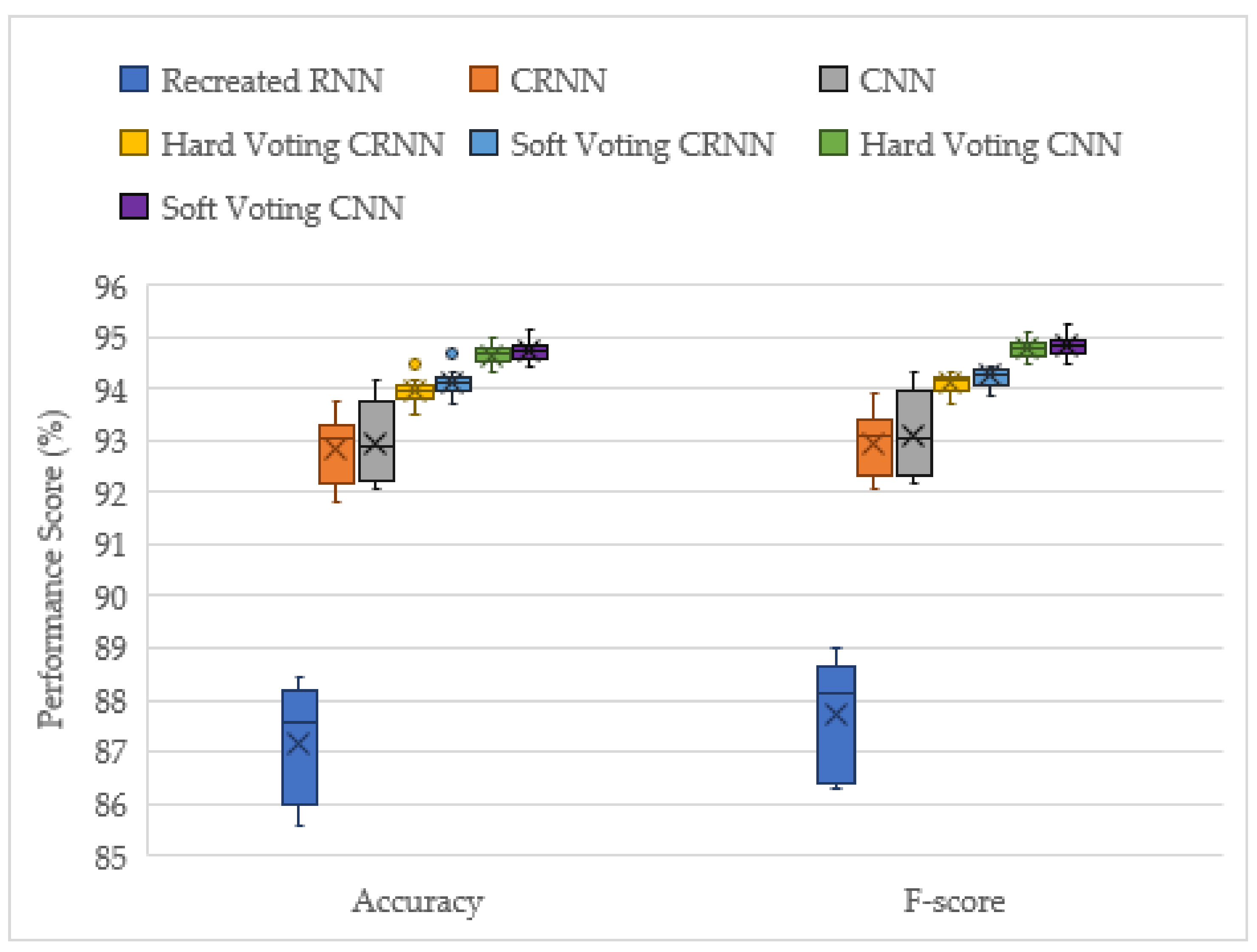
Figure 8 recaps the performance results of all models (solo and late fusion), allowing for a simple visualization of the top performing models. The corresponding performance scores are listed in Table 5, where the averaged values over 10 runs are recorded.
The late fusion models noticeably improve the classification performance in all aspects, with the soft voting CNN achieving a mean average accuracy of 94.7%, compared to the top performing solo model CNN’s average of 93.0%. Additionally, the interquartile range is significantly smaller with late fusion, showing that late fusion networks have more stable performance results compared to solo models. In conclusion, late fusion improves performance and reduces the instability of training, with the added benefit of not having to fully optimize solo model hyperparameters. The only downside with late fusion is the extra training time required to train all the voting models. However, this study does not take training time into consideration since this is dependent on the computational power available. The most important aspect is that all the models can make quick predictions. The prediction time for late fusion models is comparable with the solo models.
3.4. Top Performing Models on Real-World Unseen Dataset
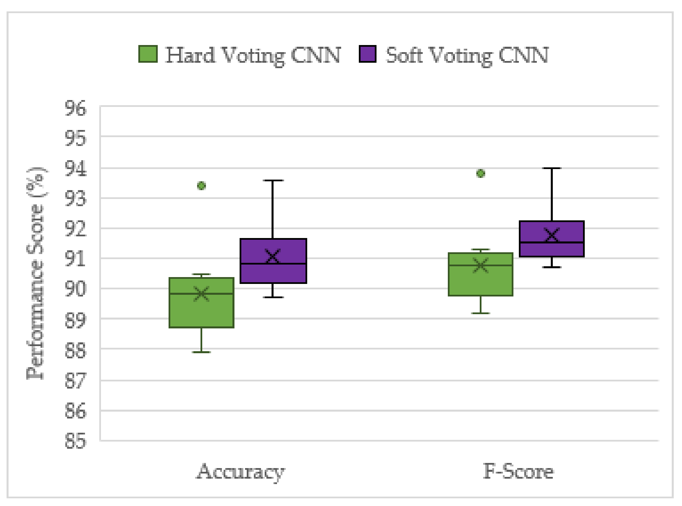
All models discussed in this study have been tested on the unseen augmented dataset simulating a UAV hovering over an airport, because it was not possible to record a real UAV flying within an airport’s perimeter. However, for a proof of concept, real-world audios, as described in Section 2.1.2, were also used to verify that the model would work in real settings. Figure 9 shows the CNN late fusion network achieving a reasonably good performance against the unseen real-world testing dataset, with high accuracy and F-scores. The corresponding averaged performance scores are listed in Table 6.
4. Conclusions
This project has demonstrated the effectiveness of ensemble deep learning models for the acoustic identification of multirotor UAVs, which achieved classification accuracies as high as 94.7 and 91.0% from the unseen augmented and real-world testing datasets, respectively. The investigation conducted on the optimized solo model architectures resulted in the CNN and CRNN models outperforming the recreated top performing model from [16], an RNN model. In this study, the acoustic signals were transformed into mel-spectrograms, and CNNs have been shown to be the best suited for image processing tasks. The solo CNN model performs slightly better than the CRNN, but it has more instability in its results. Furthermore, when late fusion was used, the CNN voting ensemble significantly outperformed the CRNN ensemble, and the CRNNs stability advantage was lost. Hence, both the reported advantages of the CRNN models [15] were not found in late fusion, and the CNN model was shown to be the best suited for this acoustic UAV detection application.
This study has also shown that late fusion networks do not require optimal hyperparameters to work well, as arbitrary hyperparameters were used, yet their performance was higher compared to the solo models with optimized hyperparameters. In addition, the instability of the performance results was significantly reduced with late fusion. The only drawback of using late fusion networks is that they take significantly more time to train, since they have more than one model requiring training (ten in this case). However, time matters more when the models are making predictions. Once all the models are trained, the prediction time remains negligible.
The distance between a drone and a microphone is a limiting factor that affects detection performance. Hence, for future work, it would be useful to study at what distances the drone would no longer be detected, and how to optimize the arrangement of microphones around an airport’s perimeter to ensure that the drones can always be detected within a certain radius. This would also lead to acoustically localizing the UAV for taking countermeasures. Flight conditions, such as hovering, low-speed and high-speed flight, are another useful factor to analyze when evaluating detection performance. Future work could evaluate model performance against different flight conditions.
While the developed framework could be applicable to other sound classification problems, such as air and road vehicles, engines and rotating machinery, the networks constructed and optimized here were specific for UAV detection, as they were trained using mel-spectrograms as inputs, representing key acoustic features of the drone/background sounds. The proposed late fusion technique could also be utilized for further work with other detection methods. It could be applied to create a voting ensemble of acoustic, radar and visual models, which would then improve the overall detection performance.
Author Contributions
Conceptualization, Y.Z. and P.C.; methodology, Y.Z. and P.C.; formal analysis, P.C.; writing—original draft preparation, P.C.; writing—review and editing, Y.Z.; supervision, Y.Z. Both authors have read and agreed to the published version of the manuscript.
Funding
This research received no external funding.
Data Availability Statement
Data and Python program used in this study can be found from GitHub repository: https://github.com/pcasabianca/Acoustic-UAV-Identification, accessed on 22 June 2021.
Conflicts of Interest
The authors declare no conflict of interest.
References
- Vemula, H.C. Multiple Drone Detection and Acoustic Scene Classification with Deep Learning. Master’s Thesis, Wright State University, Dayton, OH, USA, 2018. [Google Scholar]
- Choi-Fitzpatrick, A. Drones for Good: Technological Innovations, Social Movements, and the State. J. Int. Aff. 2014, 68, 19. [Google Scholar]
- Whelan, I. What Happens When a Drone Hits an Airplane Wing? Aviation International News, 3 October 2018. [Google Scholar]
- Geelvink, N. Drones Still a Problem Even with Little Traffic. DFS Deutsche Flugsicherung GmbH, 18 January 2021. [Google Scholar]
- DJI Mini 2. DJI. Available online: https://www.dji.com/uk/mini-2?from=store-product-page (accessed on 29 December 2020).
- Mandal, S.; Chen, L.; Alaparthy, V.; Cummings, M. Acoustic Detection of Drones through Real-Time Audio Attribute Prediction. In Proceedings of the AIAA Scitech 2020 Forum, Orlando, FL, USA, 6–10 January 2020; pp. 1–13. [Google Scholar] [CrossRef]
- Baron, V.; Bouley, S.; Muschinowski, M.; Mars, J.; Nicolas, B. Drone Localization and Identification Using an Acoustic Array and Supervised Learning. Int. Soc. Opt. Photonics 2019, 2019, 13. [Google Scholar] [CrossRef] [Green Version]
- Bernardini, A.; Mangiatordi, F.; Pallotti, E.; Capodiferro, L. Drone Detection by Acoustic Signature Identification. Electron. Imaging 2017, 2017, 60–64. [Google Scholar] [CrossRef]
- Anwar, M.Z.; Kaleem, Z.; Jamalipour, A. Machine Learning Inspired Sound-Based Amateur Drone Detection for Public Safety Applications. IEEE Trans. Veh. Technol. 2019, 68, 2526–2534. [Google Scholar] [CrossRef]
- Rabaoui, A.; Kadri, H.; Lachiri, Z.; Ellouze, N. One-Class SVMs Challenges in Audio Detection and Classification Applications. Eurasip J. Adv. Signal Process. 2008, 2008, 1–22. [Google Scholar] [CrossRef] [Green Version]
- Zahid, S.; Hussain, F.; Rashid, M.; Yousaf, M.H.; Habib, H.A. Optimized Audio Classification and Segmentation Algorithm by Using Ensemble Methods. Math. Probl. Eng. 2015, 2015, 209814. [Google Scholar] [CrossRef]
- Eklund, V. Data Augmentation Techniques for Robust Audio Analysis. Master’s Thesis, Tampere University, Tampere, Finland, 2019. [Google Scholar]
- Mezei, J.; Molnar, A. Drone Sound Detection by Correlation. In Proceedings of the SACI 2016—11th IEEE International Symposium on Applied Computational Intelligence and Informatics, Timisoara, Romania, 12–14 May; pp. 509–518. [CrossRef]
- Han, Y.; Park, J.; Lee, K. Convolutional Neural Networks with Binaural Representations and Background Subtraction for Acoustic Scene Classification. In Proceedings of the DCASE 2017-Workshop on Detection and Classification of Acoustic Scenes and Events, Munich, Germany, 16–17 November 2017; Volume 2. [Google Scholar]
- Al-Emadi, S.; Al-Ali, A.; Mohammad, A.; Al-Ali, A. Audio Based Drone Detection and Identification Using Deep Learning. In Proceedings of the 2019 15th International Wireless Communications and Mobile Computing Conference, IWCMC 2019, Tangier, Morocco, 24–28 June 2019; pp. 459–464. [Google Scholar] [CrossRef]
- Jeon, S.; Shin, J.W.; Lee, Y.J.; Kim, W.H.; Kwon, Y.H.; Yang, H.Y. Empirical Study of Drone Sound Detection in Real-Life Environment with Deep Neural Networks. In Proceedings of the 2017 25th European Signal Processing Conference (EUSIPCO), Kos, Greece, 28 August–2 September 2017; pp. 1858–1862. [Google Scholar]
- Nordby, J. Audio Classification Using Machine Learning. In Proceedings of the EuroPython Conference, Basel, Switzerland, 8–14 July 2019. [Google Scholar] [CrossRef]
- Zhang, Y.; Martinez-Garcia, M.; Latimer, A. Selecting Optimal Features for Cross-Fleet Analysis and Fault Diagnosis of Industrial Gas Turbines. In Proceedings of the ASME Turbo Expo 2018: Turbomachinery Technical Conference and Exposition, Oslo, Norway, 11–15 June 2018. [Google Scholar] [CrossRef]
- Purwins, H.; Li, B.; Virtanen, T.; Schlüter, J.; Chang, S.Y.; Sainath, T. Deep Learning for Audio Signal Processing. IEEE J. Sel. Top. Signal Process. 2019, 13, 206–219. [Google Scholar] [CrossRef] [Green Version]
- Choi, K.; Fazekas, G.; Sandler, M.; Cho, K. A Comparison of Audio Signal Preprocessing Methods for Deep Neural Networks on Music Tagging. In Proceedings of the 2018 26th European Signal Processing Conference (EUSIPCO), Rome, Italy, 3–7 September 2018; pp. 1870–1874. [Google Scholar] [CrossRef] [Green Version]
- Li, J.; Dai, W.; Metze, F.; Qu, S.; Das, S. A Comparison of Deep Learning Methods for Environmental Sound Detection. In Proceedings of the 2017 IEEE International conference on acoustics, speech and signal processing (ICASSP), New Orleans, LA, USA, 5–9 March 2017. [Google Scholar]
- Martinez-Garcia, M.; Zhang, Y.-D.; Suzuki, K.; Zhang, Y.-D. Deep Recurrent Entropy Adaptive Model for System Reliability Monitoring. IEEE Trans. Ind. Inform. 2021, 17, 839–848. [Google Scholar] [CrossRef]
- Shao, H.; Xia, M.; Han, G.; Zhang, Y.; Wan, J. Intelligent Fault Diagnosis of Rotor-Bearing System Under Varying Working Conditions with Modified Transfer Convolutional Neural Network and Thermal Images. IEEE Trans. Ind. Inform. 2021, 17, 3488–3496. [Google Scholar] [CrossRef]
- Bergstra, J.; Casagrande, N.; Erhan, D.; Eck, D.; Kégl, B. Aggregate Features and ADABOOST for Music Classification. Mach. Learn. 2006, 65, 473–484. [Google Scholar] [CrossRef]
- Xie, J.; Zhu, M. Handcrafted Features and Late Fusion with Deep Learning for Bird Sound Classification. Ecol. Inform. 2019, 52, 74–81. [Google Scholar] [CrossRef]
- Du Boisberranger, J.; van den Bossche, J.; Estève, L.; Fan, T.J.; Gramfort, A.; Grisel, O.; Halchenko, Y.; Hug, N.; Jalali, A.; Lemaitre, G.; et al. Scikit-Learn. Available online: https://scikit-learn.org/stable/about.html (accessed on 17 June 2021).
- Abadi, M.; Barham, P.; Chen, J.; Chen, Z.; Davis, A.; Dean, J.; Devin, M.; Ghemawat, S.; Irving, G.; Isard, M.; et al. TensorFlow: A System for Large-Scale Machine Learning. In Proceedings of the 12th USENIX Symposium on Operating Systems Design and Implementation (OSDI 16) 2016, Savannah, GA, USA, 2–4 November 2016. [Google Scholar]
- McFee, B.; Raffel, C.; Liang, D.; Ellis, D.; McVicar, M.; Battenberg, E.; Nieto, O. Librosa: Audio and Music Signal Analysis in Python. In Proceedings of the 14th python in science conference 2015, Austin, TX, USA, 6–12 July 2015; pp. 18–24. [Google Scholar] [CrossRef] [Green Version]
- Svanstrm, F.; Englund, C.; Alonso-Fernandez, F. Real-Time Drone Detection and Tracking with Visible, Thermal and Acoustic Sensors. In Proceedings of the 2020 25th International Conference on Pattern Recognition (ICPR), Milan, Italy, 10–15 January 2020. [Google Scholar]
- Sigtia, S.; Dixon, S. Improved Music Feature Learning with Deep Neural Networks. In Proceedings of the 2014 IEEE International Conference on Acoustics, Speech and Signal Processing (ICASSP), Florence, Italy, 4–9 May 2014. [Google Scholar]
- Rahul, R.K.; Anjali, T.; Menon, V.K.; Soman, K.P. Deep Learning for Network Flow Analysis and Malware Classification. In Proceedings of the International Symposium on Security in Computing and Communication, Manipal, India, 13–16 September 2017; pp. 226–235. [Google Scholar] [CrossRef]
- Masters, D.; Luschi, C. Revisiting Small Batch Training for Deep Neural Networks. arXiv 2018, arXiv:1804.07612. [Google Scholar]
- Goodfellow, I.; Bengio, Y.; Courville, A. Deep Learning; MIT Press: London, UK, 2016. [Google Scholar]
Figure 1.
Workflow diagram from data preparation to model training and evaluation.

Figure 2.
Real world testing data collection setup. Audio was recorded using an iPhone 11 Pro, placed on the orange mat after the take-off of the DJI Mini 2 drone.
Figure 2.
Real world testing data collection setup. Audio was recorded using an iPhone 11 Pro, placed on the orange mat after the take-off of the DJI Mini 2 drone.

Figure 3.
Mel-spectrograms, used in the training dataset, of (a) 10 s Parrot Mambo drone audio; (b) 10 s plane background audio; (c) 10 s Parrot Mambo drone (from (a)) artificially mixed with 10 s plane background audio (from (b)).
Figure 3.
Mel-spectrograms, used in the training dataset, of (a) 10 s Parrot Mambo drone audio; (b) 10 s plane background audio; (c) 10 s Parrot Mambo drone (from (a)) artificially mixed with 10 s plane background audio (from (b)).

Figure 4.
Training history of a CNN model; cross-entropy loss vs. training epoch.

Figure 5.
t-SNE visualization of the training dataset as (a) input for training model and (b) output from the trained model.
Figure 5.
t-SNE visualization of the training dataset as (a) input for training model and (b) output from the trained model.

Figure 6.
Solo RNN, CRNN and CNN model performance evaluation for ten training and testing runs, with box plots and indicating the mean value.
Figure 6.
Solo RNN, CRNN and CNN model performance evaluation for ten training and testing runs, with box plots and indicating the mean value.

Figure 7.
Hard and weighted soft voting (CRNN and CNN) performance results for ten training and testing runs, with box plots and indicating the mean value.
Figure 7.
Hard and weighted soft voting (CRNN and CNN) performance results for ten training and testing runs, with box plots and indicating the mean value.

Figure 8.
Performance results of all solo and late fusion models after ten training and testing runs, with box plots and indicating the mean value.
Figure 8.
Performance results of all solo and late fusion models after ten training and testing runs, with box plots and indicating the mean value.

Figure 9.
Performance results of hard and soft voting CNN models against a real-world unseen dataset, with box plots and indicating the mean value.
Figure 9.
Performance results of hard and soft voting CNN models against a real-world unseen dataset, with box plots and indicating the mean value.


Table 1.
Breakdown of the different datasets used and their sizes (in seconds). Background audios consist of planes, helicopters, traffic, thunderstorms, wind and quiet settings.
Table 1.
Breakdown of the different datasets used and their sizes (in seconds). Background audios consist of planes, helicopters, traffic, thunderstorms, wind and quiet settings.
| Dataset | Class | Audio | Time (s) | Total Time (s) |
|---|---|---|---|---|
| Training | UAV | Multirotor UAV-1 | 3410 | 39,940 |
| Multirotor UAV-1 + Background-1 | 16,560 | |||
| No UAV | Background-1 | 16,560 | ||
| Extra Background-2 | 3410 | |||
| Unseen Augmented Testing | UAV | DJI Mini 2 drone + Background-3 | 12,810 | 51,240 |
| RED5 drone + Background-3 | 12,810 | |||
| No UAV | Background-3 | 12,810 | ||
| Extra Background-4 | 12,810 | |||
| Unseen Real-World Testing | UAV | DJI Mini 2 drone with a helicopter flying over | 60 | 546 |
| DJI Mini 2 drone near a road | 213 | |||
| No UAV | Same road | 273 |
Table 2.
Optimized CNN architecture.
| Layer Type | Kernels | Kernel Size | Kernel Stride Size | # of Neurons | Rate | Activation |
|---|---|---|---|---|---|---|
| 2D Convolutional | 8 | 5 5 | - | - | - | ReLU |
| 2D Max Pooling | - | 5 5 | 2 | - | - | - |
| Batch Normalization | - | - | - | - | - | - |
| 2D Convolutional | 32 | 5 5 | - | - | - | ReLU |
| 2D Max Pooling | - | 5 5 | 2 | - | - | - |
| Batch Normalization | - | - | - | - | - | - |
| Flatten | - | - | - | - | - | - |
| Dense | - | - | - | 32 | - | ReLU |
| Dropout | - | - | - | - | 0.3 | - |
| Dense (Output) | - | - | - | 2 | - | Softmax |
Table 3.
Optimized CRNN architecture.
| Layer Type | Kernels | Kernel Size | Kernel Stride Size | Memory Units | # of Neurons | Rate | Activation |
|---|---|---|---|---|---|---|---|
| 2D Convolutional | 16 | 5 5 | - | - | - | - | ReLU |
| 2D Max Pooling | - | 5 5 | 2 | - | - | - | - |
| Batch Normalization | - | - | - | - | - | - | - |
| Reshape for LSTM | - | - | - | - | - | - | - |
| LSTM | - | - | - | 32 | - | - | - |
| Flatten | - | - | - | - | - | - | - |
| Dense | - | - | - | - | 32 | ReLU | |
| Dropout | - | - | - | - | - | 0.4 | - |
| Dense (Output) | - | - | - | - | 2 | - | Softmax |
Table 4.
Adapted RNN architecture from Jeon et al. [16].
Table 4.
Adapted RNN architecture from Jeon et al. [16].
| Layer Type | Memory Units | # of Neurons | Rate | Activation |
|---|---|---|---|---|
| Bidirectional LSTM | 100 | - | - | - |
| Bidirectional LSTM | 100 | - | - | - |
| Bidirectional LSTM | 100 | - | - | - |
| Dense | - | 100 | - | ReLU |
| Dropout | - | - | 0.5 | - |
| Dense (Output) | - | 2 | - | Softmax |
Table 5.
All models’ testing performance results from unseen augmented dataset.
| Score (%) | Recreated RNN | Optimised CRNN | Optimised CNN | Hard Voting CRNN | Soft Voting CRNN | Hard Voting CNN | Soft Voting CNN |
|---|---|---|---|---|---|---|---|
| Accuracy | 87.147 | 92.847 | 92.957 | 93.947 | 94.118 | 94.654 | 94.725 |
| F-score | 87.723 | 92.962 | 93.089 | 94.142 | 94.274 | 94.773 | 94.815 |
Table 6.
Testing performance results from real-world unseen dataset.
| Score (%) | Hard Voting CNN | Soft Voting CNN |
|---|---|---|
| Accuracy | 89.835 | 91.044 |
| F-score | 90.741 | 91.747 |
Publisher’s Note: MDPI stays neutral with regard to jurisdictional claims in published maps and institutional affiliations. |
© 2021 by the authors. Licensee MDPI, Basel, Switzerland. This article is an open access article distributed under the terms and conditions of the Creative Commons Attribution (CC BY) license (https://creativecommons.org/licenses/by/4.0/).
Share and Cite
MDPI and ACS Style
Casabianca, P.; Zhang, Y. Acoustic-Based UAV Detection Using Late Fusion of Deep Neural Networks. Drones 2021, 5, 54. https://0-doi-org.brum.beds.ac.uk/10.3390/drones5030054
AMA Style
Casabianca P, Zhang Y. Acoustic-Based UAV Detection Using Late Fusion of Deep Neural Networks. Drones. 2021; 5(3):54. https://0-doi-org.brum.beds.ac.uk/10.3390/drones5030054
Chicago/Turabian StyleCasabianca, Pietro, and Yu Zhang. 2021. "Acoustic-Based UAV Detection Using Late Fusion of Deep Neural Networks" Drones 5, no. 3: 54. https://0-doi-org.brum.beds.ac.uk/10.3390/drones5030054