A Hybrid Approach for Autonomous Collision-Free UAV Navigation in 3D Partially Unknown Dynamic Environments

Abstract

In the past decades, unmanned aerial vehicles (UAVs) have emerged in a wide range of applications. Owing to the advances in UAV technologies related to sensing, computing, power, etc., it has become possible to carry out missions autonomously. A key component to achieving this goal is the development of safe navigation methods, which is the main focus of this work. A hybrid navigation approach is proposed to allow safe autonomous operations in three-dimensional (3D) partially unknown and dynamic environments. This method combines a global path planning algorithm, namely RRT-Connect, with a reactive control law based on sliding mode control to provide quick reflex-like reactions to newly detected obstacles. The performance of the suggested approach is validated using simulations.

1. Introduction

Unmanned aerial vehicles (UAVs), also known as aerial drones, have emerged in many applications where it is required that some repetitive tasks are performed in a certain environment. Autonomous operation is highly desirable in these applications, which adds more requirements on the vehicle to achieve safe navigation towards areas of interest. Navigation methods can be generally classified as global path planning (deliberative), local path planning (sensor-based), and hybrid. A subset of sensor-based methods include reactive approaches [1].

Global path planning requires an overall knowledge about the environment to produce optimal and efficient paths which can be tracked by the vehicle’s control system. There exist many different techniques to address global planning problems, including roadmap methods [2,3], cell decomposition [4], potential field [5,6], probabilistic roadmap (PRM) [7], rapidly exploring random tree (RRT) [8], and optimization-based techniques [9,10,11,12]. Some of these techniques become computationally challenging when dealing with unknown and dynamic environments since a complete updated map is required a priori. As a workaround to handle such environments, extensions to some of these approaches were proposed by adding an additional layer to continuously refine the initial path locally around detected obstacles. This still may be less efficient in highly complex and dynamic environments.

On the other hand, sensor-based methods generate local paths or motion commands in real-time based on a locally observed fraction of the environment interpreted directly from sensors measurements. Search-based methods, such as those used for global planning, and optimization-based methods can be used with a local map to generate paths locally where computational complexity depends on the selected map size. On the contrary, reactive methods offer better computational solutions by directly coupling sensors observations into control inputs providing quick reactions to perceived obstacles. Hence, they can be more suitable in unknown and dynamic environments. Examples of classical reactive methods used in unknown environments are dynamic window [13] and curvature velocity [14]. Other classical examples of reactive methods dealing with dynamic obstacles include collision cones [15] and velocity obstacles [16]. A class of reactive approaches adopt a boundary following paradigm to circumvent obstructing obstacles; for examples, see [17,18,19,20,21,22,23]. The low computational cost of such methods comes at the expense of being prone to trapping situations. Some researchers suggested a combination of a randomized behavior with the boundary following approach to escape such situations [24]. However, this may sometimes produce very unpredictable motions and even inefficient ones [25] without utilizing previous sensors observation acquired through the motion.

Hybrid strategies tend to address the afromentioned drawbacks by combining both deliberative and reactive approaches for a more efficient navigation behavior in unknown and dynamic environments. There exists a body of literature on hybrid approaches; for examples, see [25,26,27,28,29,30,31] and references therein. A hybrid approach was suggested in [25] for navigation in dynamic environments which combined a potential field-based local planner with the A* algorithm as a global planner based on a topological map. Similarly, the work [26] adopted the A* algorithm with binary grid maps while using a variant of the Bug algorithm as a reactive component to address navigation in partially unknown environments. The authors of [27] suggested another hybrid approach for micro aerial vehicles that uses A* for both deliberative and local planning components where the global path gets refined locally around obstacles through replanning processes. The hybrid approach presented in [28] adopted a fuzzy logic-based boundary following technique to implement the reactive layer while an optimal reciprocal collision avoidance (ORCA) algorithm was used in [29]. Sampling-based search methods were also used in some approaches such as [30], where a global planner based on the dynamic rapidly exploring random tree (DRRT) was suggested. Real-time obstacle avoidance was then dealt with by choosing a best candidate trajectory from a sampled set. In [31], the parallel elliptic limit-cycle approach was adopted to implement both global and local planning components.

Many of the existing three-dimensional (3D) hybrid navigation methods consider search-based methods to implement the local planning component. Among those that adopt reactive-based approaches, many have just considered two-dimensional methods by constraining UAV movement to a fixed altitude which does not utilize the full capabilities of UAVs. Therefore, the main contribution of this work is to propose a hybrid 3D navigation strategy for UAVs to allow efficient navigation in partially unknown/dynamic environments. The suggested strategy combines a global path planning layer with a reactive obstacle avoidance control law developed based on a general 3D kinematic model. The global path planning layer, based on RRT-Connect, can produce efficient paths based on the available knowledge about the environment. The sliding mode technique is adopted to implement a boundary following behavior in the reactive layer. This choice provides quick reactions to obstacles with a cheap computational cost compared to search-based and optimization-based local planners. To develop a proper hybrid navigation strategy, implementation of a switching mechanism is presented to handle the transition between the two control laws. Overall, the proposed method can overcome the shortcomings of relying purely on a deliberative or reactive approaches.

This paper is organized as follows. Section 2 provides a formulation of the tackled navigation problem. The suggested hybrid strategy is then presented in Section 3. The performance of this approach is confirmed through different simulation scenarios, which is shown in Section 4. Finally, concluding remarks are made in Section 5.

2. Problem Statement

A general 3D navigation problem is considered here, where a UAV is required to navigate safely in a partially known environment $\mathcal{E}\subset {\mathbb{R}}^3$. The environment $\mathcal{E}$ contains a set of n obstacles $\mathcal{O}=\{{\mathcal{O}}_1,{\mathcal{O}}_2,\dots ,{\mathcal{O}}_n\}\subset \mathcal{E}$. These obstacles can either be static and known ${\mathcal{O}}^k$ or unknown static/dynamic ${\mathcal{O}}^u$ such that $\mathcal{O}={\mathcal{O}}^k\cup {\mathcal{O}}^u$. The main objective is to safely guide the UAV to reach some goal position ${\mathit{p}}_{goal}\in \mathcal{E}\setminus \left\{\mathcal{O}\right\}$ represented in a world coordinate frame $\mathcal{W}$ with obstacle avoidance capability. The UAV starts with an initial map of the environment containing only information about ${\mathcal{O}}^k$ based on previous knowledge. Unknown environments can also be considered where the UAV can start building a map as it traverses the environment. In this case, ${\mathcal{O}}^k=\varnothing$ initially. In addition, let $\mathit{p}\left(t\right)={[x\left(t\right),y\left(t\right),z\left(t\right)]}^T$ be the UAV Cartesian coordinates expressed in $\mathcal{W}$. Note that we represent vector quantities as column vectors; however, they can be written as the transpose of row vectors ${[·]}^T$ to simplify writing. A safety requirement for the UAV is defined as keeping a safe distance $d_{safe}>0$ from all obstacles according to the following:

$$d\left(t\right):=\underset{{\mathit{p}}^{\prime }\left(t\right)\in \mathcal{O}}{min}\left|\right|\mathit{p}\left(t\right)-{\mathit{p}}^{\prime }\left(t\right)\left|\right|\ge d_{safe}\forall t$$

(1)

where $d\left(t\right)$ is the distance to the closest obstacle, and $\left|\right|·\left|\right|$ is the standard Euclidean norm of a vector in ${\mathbb{R}}^3$.

We consider a general 3D nonholonomic kinematic model which is applicable to different types of UAVs and autonomous underwater vehicles. A description of this model is given as follows:

$$\begin{array}{ccc}\hfill \dot{\mathit{p}}\left(t\right)& =& V\left(t\right)\mathit{r}\left(t\right)\hfill \end{array}$$

(2)

$$\begin{array}{ccc}\hfill \dot{\mathit{r}}\left(t\right)& =& \mathit{u}\left(t\right)\hfill \end{array}$$

(3)

$$\begin{array}{ccc}\hfill \mathit{r}\left(t\right)·\mathit{u}\left(t\right)& =& 0\hfill \end{array}$$

(4)

where $V\left(t\right)\in {\mathbb{R}}^{+}$ is the linear speed, and $\mathit{u}\left(t\right)\in {\mathbb{R}}^3$ is a 2 degree-of-freedom (DOF) control input related to angular velocity. The motion direction at any given time instant t (i.e., orientation) is characterized by a unit vector $\mathit{r}\left(t\right)$. The condition (4) indicates that the input $\mathit{u}\left(t\right)$ is always perpendicular to $\mathit{r}\left(t\right)$ which generates a steering-like behavior in 3D. The UAV velocities $V\left(t\right)$ and $\mathit{u}\left(t\right)$ are regarded as control inputs with some upper bounds (denoted by $V_{max},u_{max}>0$) due to physical limitation. These constraints can be expressed as follows:

$$\begin{array}{cc}\hfill 0\le V\left(t\right)& \le V_{max}\hfill \\ \hfill \left|\right|\mathit{u}\left(t\right)\left|\right|& \le u_{max}\hfill \end{array}$$

(5)

Notice that we consider only forward motions by not allowing negative values for $V\left(t\right)$. For constant-speed applications, $V\left(t\right)$ is kept constant at some value $\overline{V}>0$. Additionally, the following assumptions are made.

Assumption 1.

The UAV senses a fraction of the surroundings by onboard sensors, and it can determine the distance to closest obstacle as part of its perception system. An abstract sensing model is considered where obstacles within a distance of $d_{sensing}>0$ from the UAV can be detected, and bounding geometric primitive can be used to represent the sensed fraction of the object (ex. box, sphere, cylinder, and/or ellipsoid).

Assumption 2.

Estimates of the UAV’s position $\mathit{p}\left(t\right)$ and orientation vector $\mathit{r}\left(t\right)$ are available.

The following statement summarizes the considered problem in this work.

Problem 1.

Consider a UAV whose motion can be described by the model (2)–(4). Under Assumptions 1 and 2, design control laws for $V\left(t\right)$ and $\mathit{u}\left(t\right)$ to ensure a collision-free navigation through an unknown or partially known environment $\mathcal{E}$ to reach a goal position ${\mathit{p}}_{goal}$ by satisfying the safety requirement in (1) and the constraints in (5).

Remark 1.

The model (2)–(4) can be applicable to fixed-wing UAVs, multi-rotor UAVs, and autonomous underwater vehicles.

3. Proposed Hybrid Navigation Strategy

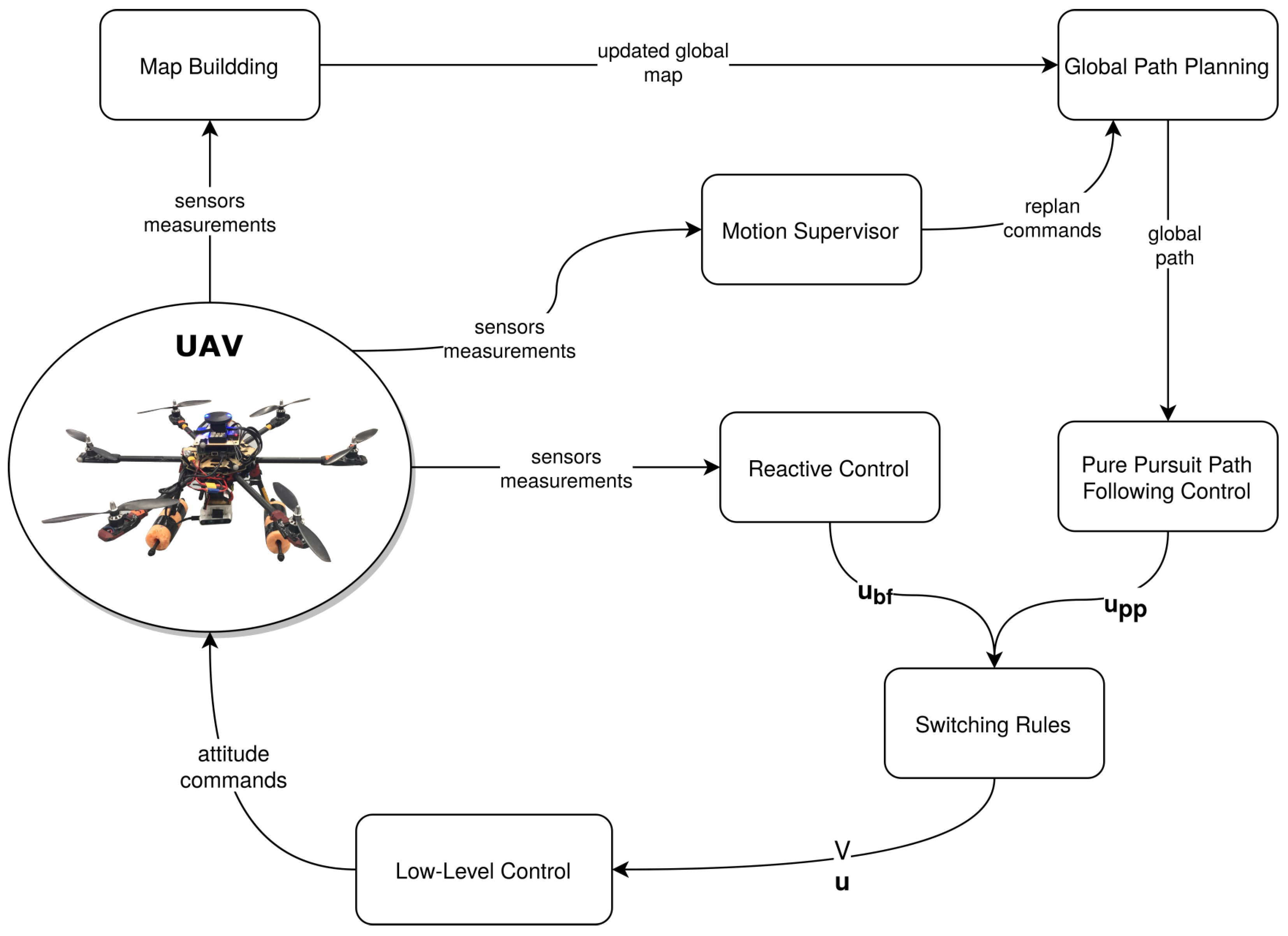
Generally, the design of autonomous navigation methods adopts modular structures. The suggested structure in this work for the overall system from a software perspective includes subsystems for perception, high-level navigation, and low-level control. The perception subsystem is responsible for processing onboard sensor measurements to provide meaningful information about the environment. Thus, it can generate an updated global map representation of the environment as well as providing distance and direction to the closest obstacle as required by our reactive control law.

The design of the high-level navigation subsystem is the main contribution of this work, and the proposed design combines a few main components, namely global path planning, motion supervisor, path following control, reactive control, and a switching mechanism. The architecture of the overall hybrid navigation strategy showing these components is presented in Figure 1.

The global path planning component is responsible for generating feasible and safe geometric paths based on the currently available global map. It is triggered to generate new paths by the motion supervisor whenever a new goal position is assigned or whenever a trapping situation (i.e., the UAV gets stuck) is detected as new portions of the environment are discovered. Initially, the map can be empty in unknown environments or partially filled in the case of partially known environments. As the vehicle navigates through the environment, the perception system updates the map based on sensors measurements. To execute the planned global paths, a path following control is adopted based on the pure pursuit guidance laws.

In unknown and dynamic environments, the vehicle may find that the planned global paths are unsafe due to the detection of new obstacles. In order to provide quick responses, a reactive control component is used to generate locally safe motions around unknown/dynamic obstacles by directly coupling command velocities into current sensors observations. The quick reactions to obstacles provided by reactive control is due to its low computational cost compared to replanning new paths. A mechanism is then used to switch between both path following and reactive navigation modes based on sensors measurements.

A detailed description of these components is given in the following subsections.

Note that the high-level navigation can normally be implemented on an onboard mission computer. The mission computer is normally connected to a Flight control unit (FCU) which is directly connected to all motors. A low-level control subsystem is then used to generate actuators/motors commands to execute the high-level velocity commands generated by the high-level navigation subsystem.

3.1. Global Path Planning

A global path planning algorithm requires a map representation of the environment. There exist many algorithms in the literature where the choice of appropriate method can vary according to the UAV sensing and computing capabilities. Optimality of the planned paths and the computational complexity of the overall algorithm could be key factors in determining which method to consider for a specific application. Note that it is also possible to adopt more than one path planning algorithm where each planner is used under certain conditions. A typical example for this case is the use of optimization-based algorithms to initially generate optimal paths while implementing a computationally efficient algorithm to modify the initial path when replanning is needed.

Our proposed hybrid navigation strategy is not restricted to a specific path planning algorithm. However, this work considers a sampling-based approach as a backbone for implementing the global planner which scales very well when planning in three-dimensional spaces. Namely, a variant of the rapidly exploring random tree (RRT) algorithm is used, which is called RRT-Connect [32]. This choice is due to the algorithm’s popularity and low computational cost which is favorable since online replanning might be needed during the motion whenever trapping scenarios are detected. Moreover, we follow an optimistic approach in our implementation of the RRT-Connect algorithm where unknown space is considered to be unoccupied (i.e., obstacle-free). Based on this assumption, the reactive controller will be responsible for handling obstacle avoidance whenever an unknown space is found to be occupied.

RRT algorithms are randomized sampling-based path planning methods which can find collision-free paths if exist with a probability that will reach one as the runtime increases (i.e., probabilistically complete). In practice, these algorithms can provide quick solutions. The basic concept of an RRT planner can be summarized as follows. Let $\mathcal{G}$ be a search tree (a graph) initialized with an initial configuration (defined later). An iterative approach is used to extend the search tree through the configuration space until a feasible solution is found. At each iteration, a configuration is sampled either randomly or using some heuristics which can help biasing the growth of the search tree. Biasing the sampling process to select the goal configuration with some probability ($0<p{b}_{goal}<1$) was found to enhance RRT growth. The algorithm then tries to extend the search tree $\mathcal{G}$ to the sampled configuration by connecting it to the nearest one within the tree. Different methods could be used to connect configurations within the configuration space especially when trying to satisfy some constraints. However, a common approach is to use straight lines to connect two configurations especially when dealing with Euclidean spaces which is considered here. A collision checker is then used to check the feasibility of each extension based on the available environment map where each feasible extension results in growing the search tree by adding the new configuration. The sampling process gets repeated iteratively until a feasible path between the initial and goal configurations is found or until a stopping criteria is met (for example, exceeding a predefined planning time limit).

RRT-Connect follows the same idea; however, it maintains two trees originating from both initial and goal configurations. At each iteration, the planner attempts to extend one of the trees followed by an attempt to find a collision-free connection to one of the vertices in the other tree. This can provide rapid convergence to a solution in complex environments compared to the standard RRT algorithm.

Due to the sampling nature of RRT algorithms, the generated paths are non-optimal in terms of the overall length. Furthermore, these paths do not satisfy nonholonomic constraints if straight lines were considered when extending the search tree. Therefore, we follow a common practice by refining the obtained paths through two post-processing stages, namely pruning and smoothing, as was done in [33,34].

For the pruning stage, redundant waypoints are removed from the planned path to improve the overall path quality. Let $W=\{w_1,w_2,\dots ,w_k\}$ be a set of waypoints representing a path generated by RRT-Connect, and let $W_p$ be the pruned path obtained after this stage. Redundant waypoints can then be removed using Algorithm 1 based on [33].

Algorithm 1 RRT Path Prunning

Input: $W=\{w_1,w_2,\dots ,w_k\}$ Output: $W_p$ 1: $W_p\leftarrow \left\{\right\}$                         ▹$W_p$ is initialized as an empty list 2: $i\leftarrow k$ 3: insert $w_i$ into $W_p$ 4: repeat 5:     $j\leftarrow 0$ 6:     repeat 7:         $j\leftarrow j+1$ 8:     until collisionFree($w_i,w_j$) or $j=i-1$     ▹ Stop when a collision-free segment is found 9:     insert $w_j$ into $W_p$ 10:     $i\leftarrow j$ 11: until i = 1

A smoothing algorithm is applied next to the pruned path to ensure that the final path satisfies the vehicle’s nonholonomic constraints (minimum radius of curvature). To that end, parametric Bezier curves were used to generate continuous-curvature smooth paths following the approach suggested in [34].

3.2. Pure Pursuit Path Following Control

A path following control design is needed to ensure that the UAV can accurately track the planned path. The proposed design adopts the pure pursuit tracking (PP) algorithm which is known for its stability and simplicity [35]. Assuming that a geometric path $\tau \subset {\mathbb{R}}^3$ is available, the PP algorithm steers the vehicle to follow a virtual target ${\mathit{p}}_v=(x_v,y_v,z_v)\in \tau$ moving along the path. This target is usually selected to be at some lookahead distance L away from the closest path point ${\mathit{p}}_c\in \tau$ to the vehicle’s current position. For more stability, a modified version of the PP algorithm is considered in this work based on [36] which suggested using an adaptive lookahead distance instead of a fixed value. This PP variant provides more stability when the vehicle is further from the planned path which is needed here since the vehicle can sometimes deviate from the planned path when avoiding obstacles with the reactive control component. The following control law is used for path following:

$$\begin{array}{ccc}\hfill V_{pp}\left(t\right)& =& V_{max}tanh\left(\gamma \Vert {\mathit{p}}_v\left(t\right)-\mathit{p}\left(t\right)\Vert \right)\hfill \end{array}$$

(6)

$$\begin{array}{ccc}\hfill {\mathit{u}}_{pp}\left(t\right)& =& u_{max}F(\mathit{r}\left(t\right),\frac{{\mathit{p}}_v\left(t\right)-\mathit{p}\left(t\right)}{\Vert {\mathit{p}}_v\left(t\right)-\mathit{p}\left(t\right)\Vert })\hfill \end{array}$$

(7)

where $\gamma >0$. The mapping function $F({\mathit{w}}_1,{\mathit{w}}_2):{\mathbb{R}}^3\times {\mathbb{R}}^3\to {\mathbb{R}}^3$ acts as a steering function which produces a vector that is perpendicular to ${\mathit{w}}_1$ in the direction of ${\mathit{w}}_2$, and it is defined as follows:

$$F({\mathit{w}}_1,{\mathit{w}}_2)=\{\begin{array}{cc}\frac{f({\mathit{w}}_1,{\mathit{w}}_2)}{\Vert f({\mathit{w}}_1,{\mathit{w}}_2)\Vert },& \Vert f({\mathit{w}}_1,{\mathit{w}}_2)\Vert \ne 0\\ {\mathit{0}}_{3\times 1},& \Vert f({\mathit{w}}_1,{\mathit{w}}_2)\Vert =0\end{array}$$

(8)

where

$$f({\mathit{w}}_1,{\mathit{w}}_2)={\mathit{w}}_2-({\mathit{w}}_1·{\mathit{w}}_2){\mathit{w}}_1$$

3.3. Reactive Control Law

Navigation in unknown and dynamic environments requires more safety measures as the planned path from the global planner can become unsafe whenever new obstacles are detected, especially if they are dynamic. Hence, a reactive control law is used to generate reflex-like reactions to detected obstacles by navigating around them until it is safe to continue following the previously planned path.

In our implementation, we adopt a reactive control law utilizing a sliding mode control technique based on [37]. The distance to closest obstacle $d\left(t\right)$ is the only information needed to implement this controller and can be obtained from onboard sensors. This reactive control is based on a boundary following paradigm, and it is given as follows:

$$\begin{array}{ccc}\hfill V_{bf}\left(t\right)& =& V_{max}\hfill \end{array}$$

(9)

$$\begin{array}{ccc}\hfill {\mathit{u}}_{bf}\left(t\right)& =& \Gamma u_{max}sgn(\dot{d}\left(t\right)+\chi (d\left(t\right)-d_0)){\mathit{i}}_n\left(t\right)\hfill \end{array}$$

(10)

$$\begin{array}{ccc}\hfill {\mathit{i}}_n\left(t\right)& =& {\mathit{i}}_a\left(t_{*}\right)\times \mathit{r}\left(t\right)\hfill \end{array}$$

(11)

where a constant forward speed is considered, $d_0>d_{safe}>0$ is a desired distance, $\Gamma =\pm 1$ determines the avoidance maneuver direction (i.e., clockwise or counter clockwise with respect to the axis of rotation), and $sgn\left(\alpha \right)$ is the signum function. In addition, $\chi \left(\beta \right)$ is a saturation function which is defined as:

$$\chi \left(\beta \right)=\{\begin{array}{cc}\gamma \beta & if\left|\beta \right|\le \delta \\ \delta \gamma sgn\left(\beta \right)& otherwise\end{array},\gamma ,\delta >0$$

(12)

for some design parameters $\gamma ,\delta >0$. In addition, ${\mathit{i}}_a\left(t_{*}\right)$ represents an avoidance plane normal associated with a certain obstacle as explained in [37]. This normal can be different for each obstacle, and it can be determined at the time instant $t_{*}$ when a new obstacle is detected.

The reactive navigation law (9)–(10) ensures that the vehicle will maintain a fixed distance $d_0$ while navigating around the nearest obstacle under some assumptions as was mathematically proven in [20].

3.4. Switching Rules

A switching mechanism is important for hybrid navigation methods. It is responsible for deciding whether it is safe to follow the planned path or to reactively avoid a newly detected obstacle. In general, two navigation modes will be used, and a switching mechanism is adopted to switch between those two modes. The two modes are path following mode ${\mathcal{M}}_1$ (control law (6) and (7)) and obstacle avoidance/reactive mode ${\mathcal{M}}_2$ (control law (9)–(11)).

Assuming that the vehicle initially starts in mode ${\mathcal{M}}_1$, we consider the following switching rules:

R1: switch to the reactive mode ${\mathcal{M}}_2$ when the distance to the closest obstacle ${\mathcal{O}}_i$ drops below some threshold distance C (i.e., $d\left(t\right)=C$ and $\dot{d}\left(t\right)<0$).

R2: switch to the path following mode ${\mathcal{M}}_1$ from ${\mathcal{M}}_2$ when $|d\left(t\right)-d_0|<{ϵ}_0\forall i$ for some small value ${ϵ}_0>0$ and the vehicle’s heading is targeted towards the virtual target ${\mathit{p}}_v$ on the planned path which can be determined according to the following condition:

$$\left|{cos}^{-1}\left(\frac{\mathit{r}·({\mathit{p}}_v-\mathit{p})}{\Vert {\mathit{p}}_v-\mathit{p}\Vert }\right)\right|\le {ϵ}_1$$

(13)

where ${ϵ}_1>0$.

3.5. Motion Supervisor

The motion supervisor is responsible for detecting trapping situations whenever the vehicle gets stuck in a local minimum due to a newly discovered fraction of the environment. An example of such scenario can be seen when navigating in maze-like environments, concave obstacles, and/or long blocking walls [38]. The proposed approach to tackle this problem is by issuing a replanning command to the global path planner to acquire a new path based on the updated knowledge about the environment.

4. Simulation Results and Discussion

The developed hybrid navigation approach was tested using simulations considering two different cases, namely static and dynamic environments. Some knowledge about these environments were assumed to be known, a priori, to show the role of the global planner; however, the developed approach can work well even when no such knowledge is available. The RRT-Connect algorithm was implemented based on [32] to plan global paths.

The simulations were carried out using the MATLAB software running on a 2.6 GHz Intel Core i7 CPU. We considered a maximum linear speed of V = 0.75 m/s and a maximum angular velocity of $u_{max}$ = 1.75 and 2.5 rad/s for the first and second cases, respectively. The design parameters were also selected as follows: $L=0.5$, $\delta =0.5$, $\gamma =1$, $d_0=1$, and $C=2$. An arbitrary choice was made for ${\mathit{i}}_a\left(t_{*}\right)$ used in (11) which vary for each obstacle. In addition, the update rate of the control was set to be 0.01 s. A description and the results of these simulations are presented next.

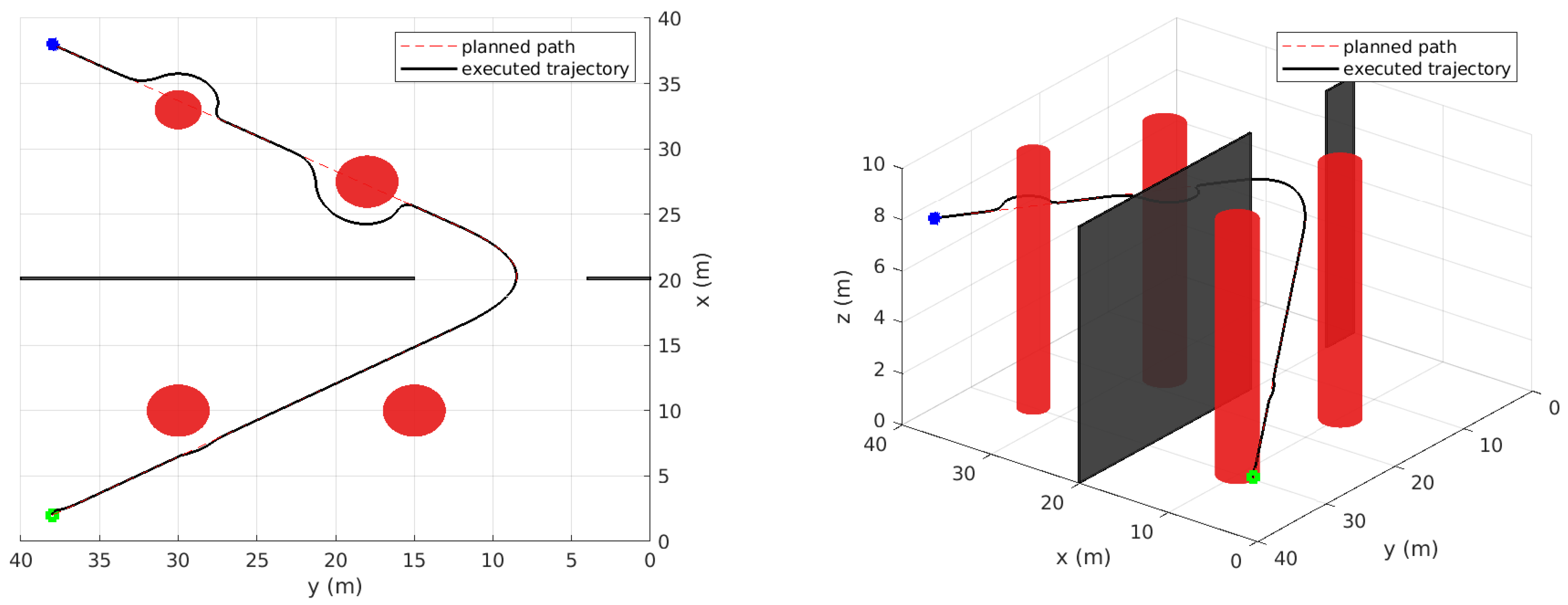
4.1. Case I: Unknown Static Obstacles

In the first simulation case, we consider an environment in which the UAV performs some repetitive tasks. Hence, some knowledge about the environment is known a priori, such as wall locations. However, new static obstacles which are not known to the vehicle can be added to the environment at different times. A real-life example of this scenario is when operating in a warehouse or inside a building. The warehouse/building layout can be known in advance or from an initial mapping process while objects can be moved around all the time.

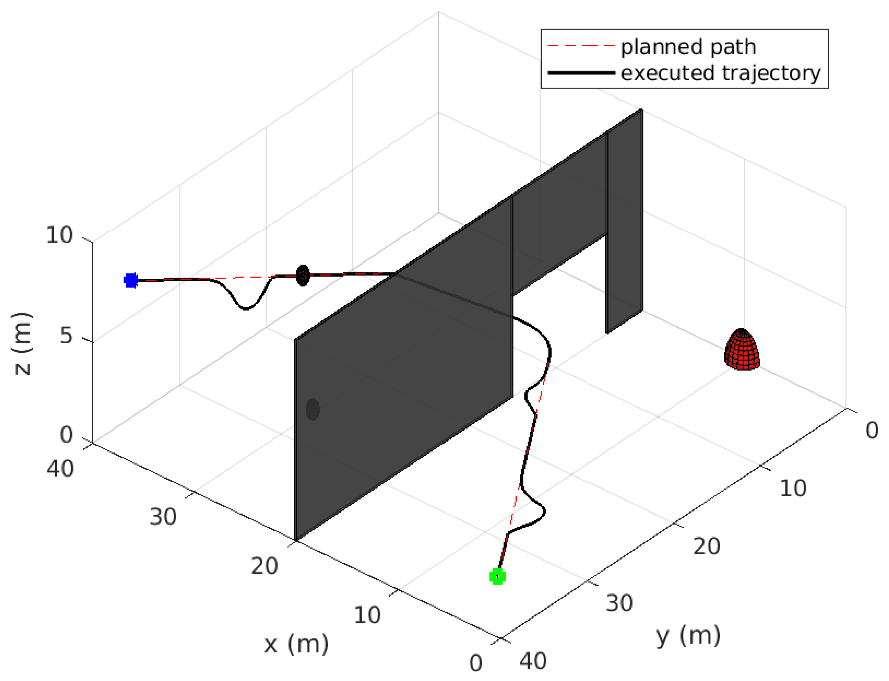
Figure 2 shows the considered environment for this simulation case. The initial map available to the vehicle includes only information about the two walls (shown in gray/black). There are also 4 unknown cylindrical shaped obstacles with different sizes. A bounding shape can usually be estimated in practice by the vehicle’s perception system to represent nearby obstacles where very close obstacles can be represented by a single bounding object to satisfy the control assumptions.

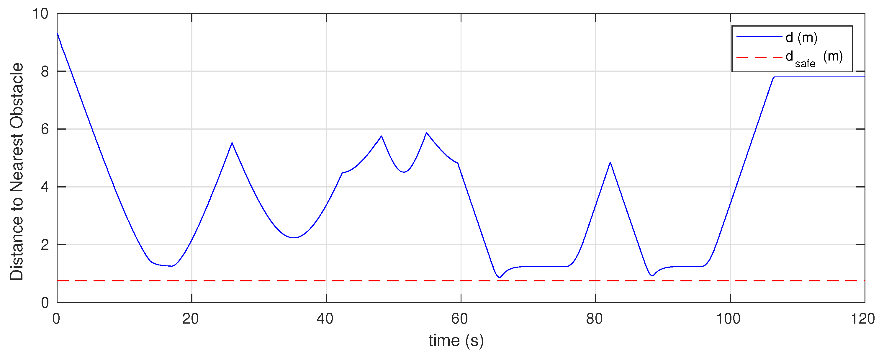
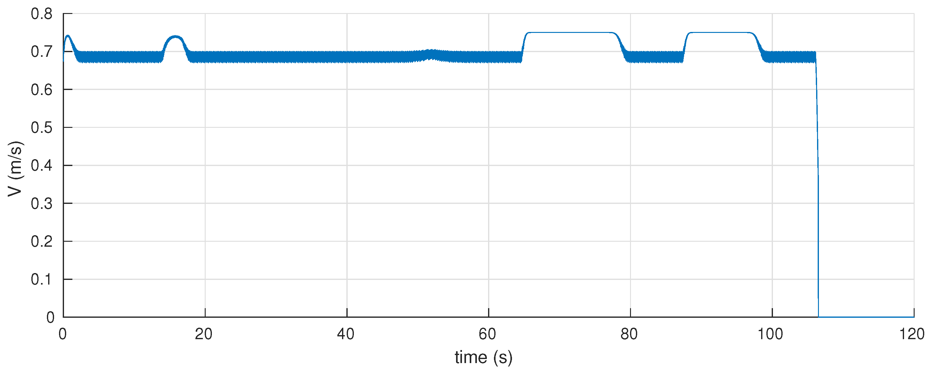
It can clearly be seen from Figure 2 that the proposed hybrid navigation strategy can safely guide the vehicle starting from some initial position (green circular marker) to reach the goal location (blue star marker). This figure shows both the path generated by the global planner based on the initial knowledge about the environment as well as the actual executed path by the vehicle. The vehicle can successfully track the planned path whenever it has good clearance from obstacles. Once an obstacle is detected by the vehicle’s sensors, the vehicle switches to the reactive mode ${\mathcal{M}}_2$ to move around the obstacle. Then, it goes back to the path following mode ${\mathcal{M}}_1$ whenever it is clear to do so according to the switching rule R2 as described earlier. The distance to the closest obstacle during the motion is given in Figure 3, which clearly shows that the vehicle can satisfy the safety requirement by maintaining a proper clearance from all obstacles. In addition, the linear speed of the vehicle is shown in Figure 4. Overall, these results confirm that the proposed method can guide the vehicle safely among unknown static obstacles.

4.2. Case II: Unknown Dynamic Obstacles

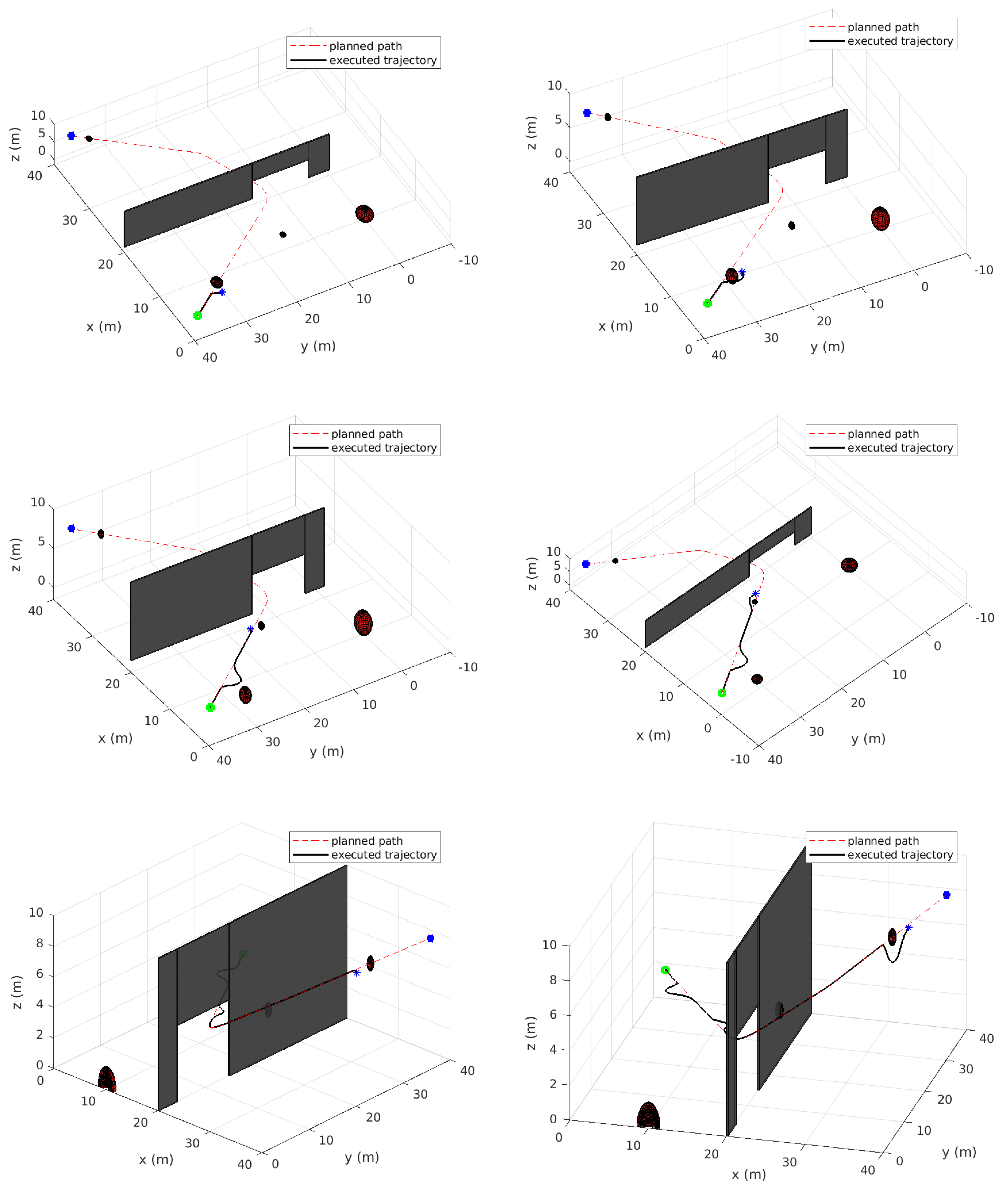
The second simulation scenario considers the case where there are several unknown moving obstacles, which makes the environment dynamic. Similar to the previous case, some initial knowledge about the environment layout is assumed to be known, which is shown in gray/black in Figure 5. Moreover, there are multiple unknown dynamic spherical obstacles with random sizes between 0.2 and 1 m in radius and arbitrary linear speeds of 0.1, 0.2, and 0.25 m/s (less than 0.75 m/s). Note that for simplicity, collisions between different obstacles are not considered in this case.

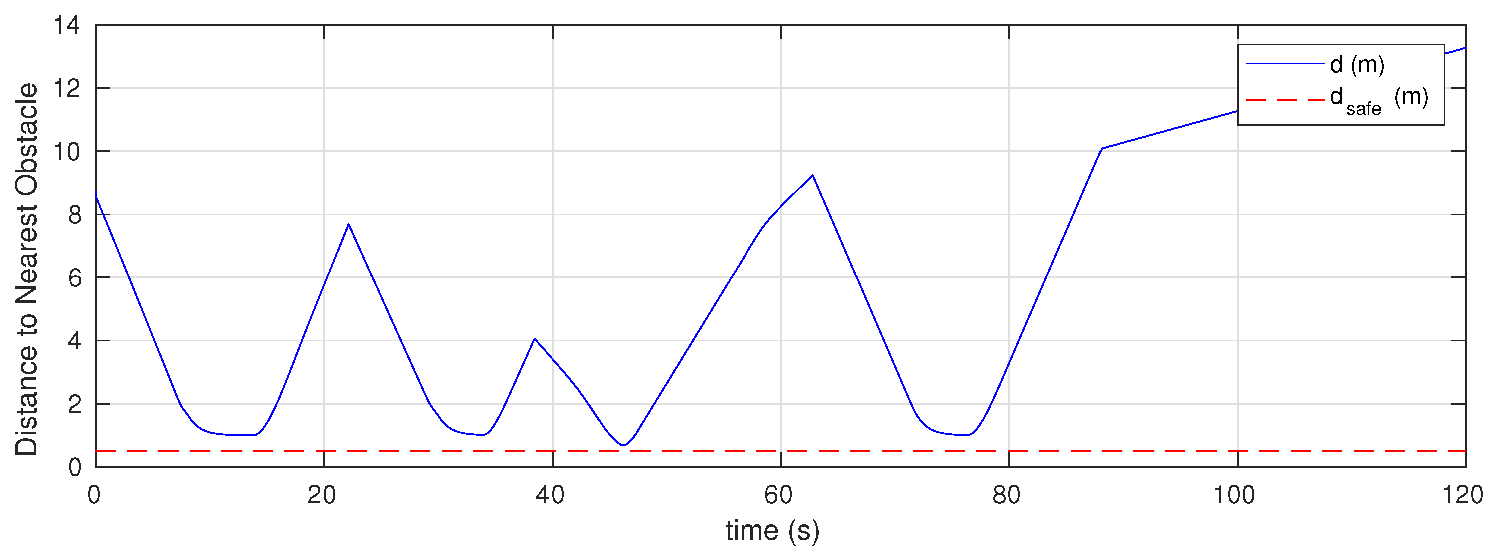
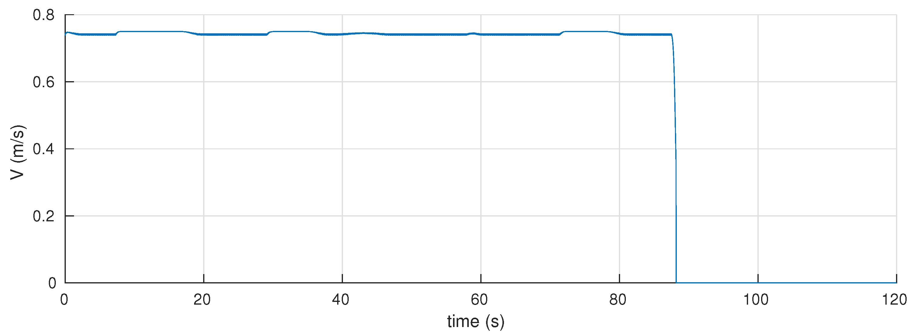
Based on the initial map, the global planner finds a safe path using RRT-Connect, which is shown as a dashed red line in Figure 5. The vehicle then starts moving in mode ${\mathcal{M}}_1$ to track the planned (reference) path. However, due to the highly dynamic nature of the environment, this path becomes unsafe whenever there are obstacles approaching the vehicle, as shown in Figure 6, at different time instants during the motion. Each time a threatening obstacle is detected, the vehicle switches to navigation in the reactive mode ${\mathcal{M}}_2$ according to the switching rule R1. This can be seen in Figure 5 and Figure 6, which show that the vehicle’s actual executed path deviates from the planned path at some locations to avoid the dynamic obstacles. This is verified in Figure 7, where the distance to the closest obstacle remain above the safety threshold. In addition, the UAV’s linear speed is shown in Figure 8. It is evident from these results that the proposed strategy also works well in dynamic environments. It should be mentioned that the UAV’s maximum velocity must be larger than obstacles’ velocities to guarantee safety. However, the reactive control law can still handle some cases where the obstacles are moving faster than the vehicle but with no safety guarantees in some aggressive scenarios.

5. Conclusions

A hybrid three-dimensional (3D) navigation strategy for unmanned aerial vehicles (UAVs) was presented in this paper. The problem formulation considered a general 3D nonholonomic kinematic model which is applicable to different UAV types and autonomous underwater vehicles. A global planner based on the RRT-Connect algorithm was used which works well in three-dimensional spaces. A reactive control law based on sliding mode control was used to avoid unknown and dynamic obstacles. Simulation results confirm that the proposed hybrid navigation method works well in 3D environments with unknown static and dynamic obstacles.

References

- Hoy, M.; Matveev, A.S.; Savkin, A.V. Algorithms for collision-free navigation of mobile robots in complex cluttered environments: A survey. Robotica 2015, 33, 463–497. [Google Scholar] [CrossRef] [Green Version]
- Lozano-Pérez, T.; Wesley, M.A. An algorithm for planning collision-free paths among polyhedral obstacles. Commun. ACM 1979, 22, 560–570. [Google Scholar] [CrossRef]
- Ó’Dúnlaing, C.; Yap, C.K. A “retraction” method for planning the motion of a disc. J. Algorithms 1985, 6, 104–111. [Google Scholar] [CrossRef]
- Lozano-Perez, T. Spatial planning: A configuration space approach. IEEE Trans. Comput. 1983, C-32, 108–120. [Google Scholar] [CrossRef] [Green Version]
- Khatib, O. Real-time obstacle avoidance for manipulators and mobile robots. Int. J. Robot. Res. 1986, 5, 90–98. [Google Scholar] [CrossRef]
- Ge, S.S.; Cui, Y.J. New potential functions for mobile robot path planning. IEEE Trans. Robot. Autom. 2000, 16, 615–620. [Google Scholar] [CrossRef] [Green Version]
- Kavraki, L.E.; Svestka, P.; Latombe, J.C.; Overmars, M.H. Probabilistic roadmaps for path planning in high-dimensional configuration spaces. IEEE Trans. Robot. Autom. 1996, 12, 566–580. [Google Scholar] [CrossRef] [Green Version]
- LaValle, S.M. Rapidly-Exploring Random Trees: A New Tool for Path Planning; The Annual Research Report; Iowa State University: Ames, IA, USA, 1998. [Google Scholar]
- Dragan, A.D.; Ratliff, N.D.; Srinivasa, S.S. Manipulation planning with goal sets using constrained trajectory optimization. In Proceedings of the 2011 IEEE International Conference on Robotics and Automation (ICRA), Shanghai, China, 9–13 May 2011; pp. 4582–4588. [Google Scholar]
- Zucker, M.; Ratliff, N.; Dragan, A.D.; Pivtoraiko, M.; Klingensmith, M.; Dellin, C.M.; Bagnell, J.A.; Srinivasa, S.S. Chomp: Covariant hamiltonian optimization for motion planning. Int. J. Robot. Res. 2013, 32, 1164–1193. [Google Scholar] [CrossRef] [Green Version]
- Schulman, J.; Duan, Y.; Ho, J.; Lee, A.; Awwal, I.; Bradlow, H.; Pan, J.; Patil, S.; Goldberg, K.; Abbeel, P. Motion planning with sequential convex optimization and convex collision checking. Int. J. Robot. Res. 2014, 33, 1251–1270. [Google Scholar] [CrossRef] [Green Version]
- Li, G.; Chou, W. Path planning for mobile robot using self-adaptive learning particle swarm optimization. Sci. China Inf. Sci. 2018, 61, 052204. [Google Scholar] [CrossRef] [Green Version]
- Fox, D.; Burgard, W.; Thrun, S. The dynamic window approach to collision avoidance. IEEE Robot. Autom. Mag. 1997, 4, 23–33. [Google Scholar] [CrossRef] [Green Version]
- Simmons, R. The curvature-velocity method for local obstacle avoidance. In Proceedings of the 1996 IEEE International Conference on Robotics and Automation, Minneapolis, MN, USA, 22–28 April 1996; Volume 4, pp. 3375–3382. [Google Scholar]
- Chakravarthy, A.; Ghose, D. Obstacle avoidance in a dynamic environment: A collision cone approach. IEEE Trans. Syst. Man Cybern. Part A Syst. Hum. 1998, 28, 562–574. [Google Scholar] [CrossRef] [Green Version]
- Fiorini, P.; Shiller, Z. Motion planning in dynamic environments using velocity obstacles. Int. J. Robot. Res. 1998, 17, 760–772. [Google Scholar] [CrossRef]
- Bemporad, A.; Di Marco, M.; Tesi, A. Sonar-Based Wall-Following Control of Mobile Robots. J. Dyn. Syst. Meas. Control 2000, 122, 226–229. [Google Scholar] [CrossRef] [Green Version]
- Toibero, J.M.; Roberti, F.; Carelli, R. Stable contour-following control of wheeled mobile robots. Robotica 2009, 27, 1–12. [Google Scholar] [CrossRef]
- Teimoori, H.; Savkin, A.V. A biologically inspired method for robot navigation in a cluttered environment. Robotica 2010, 28, 637–648. [Google Scholar] [CrossRef]
- Matveev, A.S.; Teimoori, H.; Savkin, A.V. A method for guidance and control of an autonomous vehicle in problems of border patrolling and obstacle avoidance. Automatica 2011, 47, 515–524. [Google Scholar] [CrossRef]
- Matveev, A.S.; Wang, C.; Savkin, A.V. Real-time navigation of mobile robots in problems of border patrolling and avoiding collisions with moving and deforming obstacles. Robot. Auton. Syst. 2012, 60, 769–788. [Google Scholar] [CrossRef]
- Savkin, A.V.; Wang, C. A simple biologically inspired algorithm for collision-free navigation of a unicycle-like robot in dynamic environments with moving obstacles. Robotica 2013, 31, 993–1001. [Google Scholar] [CrossRef]
- Matveev, A.; Savkin, A.; Hoy, M.; Wang, C. Safe Robot Navigation among Moving and Steady Obstacles; Elsevier: Amsterdam, The Netherlands, 2015. [Google Scholar]
- Savkin, A.V.; Hoy, M. Reactive and the shortest path navigation of a wheeled mobile robot in cluttered environments. Robotica 2013, 31, 323–330. [Google Scholar] [CrossRef]
- Urdiales, C.; Pérez, E.; Sandoval, F.; Vázquez-Salceda, J. A hybrid architecture for autonomous navigation in dynamic environments. In Proceedings of the IEEE/WIC International Conference on Intelligent Agent Technology, Halifax, NS, Canada, 13–17 October 2003. [Google Scholar]
- Zhu, Y.; Zhang, T.; Song, J.; Li, X. A new hybrid navigation algorithm for mobile robots in environments with incomplete knowledge. Knowl. Based Syst. 2012, 27, 302–313. [Google Scholar] [CrossRef]
- Nieuwenhuisen, M.; Behnke, S. Layered mission and path planning for MAV navigation with partial environment knowledge. In Intelligent Autonomous Systems 13; Springer: Berlin/Heidelberg, Germany, 2016; pp. 307–319. [Google Scholar]
- Hank, M.; Haddad, M. A hybrid approach for autonomous navigation of mobile robots in partially-known environments. Robot. Auton. Syst. 2016, 86, 113–127. [Google Scholar] [CrossRef]
- Wzorek, M.; Berger, C.; Doherty, P. A Framework for Safe Navigation of Unmanned Aerial Vehicles in Unknown Environments. In Proceedings of the 2017 25th International Conference on Systems Engineering (ICSEng), Las Vegas, NV, USA, 22–23 August 2017; pp. 11–20. [Google Scholar]
- D’Arcy, M.; Fazli, P.; Simon, D. Safe navigation in dynamic, unknown, continuous, and cluttered environments. In Proceedings of the 2017 IEEE International Symposium on Safety, Security and Rescue Robotics (SSRR), Shanghai, China, 11–13 October 2017; pp. 238–244. [Google Scholar]
- Adouane, L. Reactive versus cognitive vehicle navigation based on optimal local and global PELC*. Robot. Auton. Syst. 2017, 88, 51–70. [Google Scholar] [CrossRef]
- Kuffner, J.J.; LaValle, S.M. RRT-connect: An efficient approach to single-query path planning. In Proceedings of the 2000 ICRA, Millennium Conference, IEEE International Conference on Robotics and Automation, Symposia Proceedings (Cat. No. 00CH37065), San Francisco, CA, USA, 24–28 April 2000; Volume 2, pp. 995–1001. [Google Scholar]
- Yang, K.; Gan, S.K.; Sukkarieh, S. An Efficient Path Planning and Control Algorithm for RUAV’s in Unknown and Cluttered Environments. J. Intell. Robot. Syst. 2010, 57, 101. [Google Scholar] [CrossRef]
- Yang, K.; Sukkarieh, S. An analytical continuous-curvature path-smoothing algorithm. IEEE Trans. Robot. 2010, 26, 561–568. [Google Scholar] [CrossRef]
- Amidi, O.; Thorpe, C.E. Integrated Mobile Robot Control; Mobile Robots V. International Society for Optics and Photonics: Bellingham, WA, USA, 1991; Volume 1388, pp. 504–524. [Google Scholar]
- Giesbrecht, J.; Mackay, D.; Collier, J.; Verret, S. Path Tracking for Unmanned Ground Vehicle Navigation: Implementation and Adaptation of the Pure Pursuit Algorithm; Technical Report; Defence Research and Development Suffield: Suffield, AB, Canada, 2005.
- Elmokadem, T. A 3D Reactive Collision Free Navigation Strategy for Nonholonomic Mobile Robots. In Proceedings of the 2018 37th Chinese Control Conference (CCC), Wuhan, China, 25–27 July 2018; pp. 4661–4666. [Google Scholar]
- Nakhaeinia, D.; Payeur, P.; Hong, T.S.; Karasfi, B. A hybrid control architecture for autonomous mobile robot navigation in unknown dynamic environment. In Proceedings of the 2015 IEEE International Conference on Automation Science and Engineering (CASE), Gothenburg, Sweden, 24–28 August 2015; pp. 1274–1281. [Google Scholar]
Figure 1.
Architecture of the proposed navigation strategy.
Figure 2.
Simulation Case I: Initially planned path and executed motion (static environment).
Figure 3.
Simulation Case I: Distance from the UAV to obstacles.
Figure 4.
Simulation Case I: Linear speed of the UAV during the motion.
Figure 5.
Simulation Case II: Initial planned path and executed motion (dynamic environment).
Figure 6.
Simulation Case II: Different instances during motion at which switching to reactive mode was triggered.
Figure 7.
Simulation Case II: Distance from the UAV to obstacles.
Figure 8.
Simulation Case II: Linear speed of the UAV during the motion.
Publisher’s Note: MDPI stays neutral with regard to jurisdictional claims in published maps and institutional affiliations. |
© 2021 by the authors. Licensee MDPI, Basel, Switzerland. This article is an open access article distributed under the terms and conditions of the Creative Commons Attribution (CC BY) license (https://creativecommons.org/licenses/by/4.0/).
Share and Cite
MDPI and ACS Style
Elmokadem, T.; Savkin, A.V. A Hybrid Approach for Autonomous Collision-Free UAV Navigation in 3D Partially Unknown Dynamic Environments. Drones 2021, 5, 57. https://0-doi-org.brum.beds.ac.uk/10.3390/drones5030057
AMA Style
Elmokadem T, Savkin AV. A Hybrid Approach for Autonomous Collision-Free UAV Navigation in 3D Partially Unknown Dynamic Environments. Drones. 2021; 5(3):57. https://0-doi-org.brum.beds.ac.uk/10.3390/drones5030057
Chicago/Turabian StyleElmokadem, Taha, and Andrey V. Savkin. 2021. "A Hybrid Approach for Autonomous Collision-Free UAV Navigation in 3D Partially Unknown Dynamic Environments" Drones 5, no. 3: 57. https://0-doi-org.brum.beds.ac.uk/10.3390/drones5030057