Monitoring Onion Crop “Cipolla Rossa di Tropea Calabria IGP” Growth and Yield Response to Varying Nitrogen Fertilizer Application Rates Using UAV Imagery

Abstract

Remote sensing (RS) platforms such as unmanned aerial vehicles (UAVs) represent an essential source of information in precision agriculture (PA) as they are able to provide images on a daily basis and at a very high resolution. In this framework, this study aims to identify the optimal level of nitrogen (N)-based nutrients for improved productivity in an onion field of “Cipolla Rossa di Tropea” (Tropea red onion). Following an experiment that involved the arrangement of nine plots in the onion field in a randomized complete block design (RCBD), with three replications, three different levels of N fertilization were compared: N150 (150 kg N ha⁻¹), N180 (180 kg N ha⁻¹), and e N210 (210 kg N ha⁻¹). The crop cycle was monitored using multispectral (MS) UAV imagery, producing vigor maps and taking into account the yield of data. The soil-adjusted vegetation index (SAVI) was used to monitor the vigor of the crop. In addition, the coverage’s class onion was spatially identified using geographical object-based image classification (GEOBIA), observing differences in SAVI values obtained in plots subjected to differentiated N fertilizer treatment. The information retrieved from the analysis of soil properties (electrical conductivity, ammonium and nitrate nitrogen), yield performance and mean SAVI index data from each field plot showed significant relationships between the different indicators investigated. A higher onion yield was evident in plot N180, in which SAVI values were higher based on the production data.

1. Introduction

The International Society of Precision Agriculture (ISPAG) defines precision agriculture (PA) as “a management that gathers, processes and analyzes temporal, spatial and individual data and combines it with other information to support management decisions according to estimated variability for improved resource use efficiency, productivity, quality, profitability and sustainability of agricultural production” [1]. PA allows environmental impact costs at the farm level to be reduced through the targeted use of inputs. In addition, using agrochemicals and fertilizers more efficiently brings benefits in terms of yield and yield quality [2]. PA can be considered a cyclic system with several steps divided into data collection, data analysis, management decisions, and management decision evaluation [3]. In these frameworks, remote sensing (RS) techniques for aerial monitoring provide several solutions to collect data and map production [4]. Among the platforms, considering the differences in terms of spatial and temporal resolution, both satellites and the latest unmanned aerial vehicles (UAVs) are commonly used in PA applications. As far as satellites are concerned, nano-satellites can provide images with a relatively high temporal resolution (3 days) and a spatial resolution of about 3 m, which is useful for PA purposes [5,6]. The contribution of satellites, a significant source of RS imagery in PA [7,8], is greater than that of UAVs, providing images on a daily basis and at very high resolution below the meter. This is important for the definition of spatial variability within the field providing new tools to technicians and specialists in the management and formulation of solutions for PA, including the use and dosage of agrochemicals and fertilizers [9]. The onion (Allium cepa L.), an herbaceous biennial bulb crop of the Amaryllidaceae family, is one of the most widely cultivated and known vegetable crops [10,11]; after tomatoes, it is the most economically important crop in both world and local markets [12,13]. The root system comprises numerous fasciculated and superficial roots that grow, usually in the first 20–25 cm of soil. The bulb, the edible part with variable shape, comes from the enlargement of the basal portion of the leaves inserted and superimposed in a central cauline axis [14]. The growth and yield of cultivated plants are mainly influenced by two factors: genetic and management [15]. While the first factor is related to the various breeding techniques for improving crop varieties, the second factor includes the planting date, spacing, fertilization practices, irrigation, cultivation, weed control, and plant protection from biotic and abiotic stress factors [12,15]. Additionally, the influence of climate, soil type and soil fertility can impact productivity [16]. Among the nutrients, nitrogen (N) performs a critical role, making up about 80% of the total mineral nutrients absorbed by plants; it is crucial in photosynthesis and several physiological and biochemical reactions in plant metabolism, such as proteins, enzymes, amino acids and amides, nucleic acids, and plant hormones [17,18,19]. Its correct and effective use is fundamental for the overall sustainability of cultivation systems and a fruitful fate of this nutrient [20]. Due to their shallow, unbranched root system, onions are more susceptible to nutrient deficiencies than most crops [21]. As a consequence, this crop needs and responds well to the addition of fertilizers, especially nitrogenous ones. The management of N fertilizers in onion cultivation can improve their quality, particularly the bulb size and shelf life, with positive economic effects for farms [22]. At the same time, the efficient management of N inputs reduces the negative impact that its leaching in the form of nitrates may have on the environment; it can be a very damaging process in highly specialized districts where onions are typically grown on sandy soils, characterized by low nutrient retention and high permeability, near riparian or coastal areas, exposed to a significant risk of groundwater quality degradation and surface-water eutrophication. Sustainable onion fertilization can be achieved by choosing the appropriate formulation, correct application times and doses necessary for the crop, aiming to increase the productivity while respecting the nutrient requirements linked to optimal yield with less economic loss and minimal nutrient dispersion in the environment [23]. RS techniques applied to onion crops could help the management of several field operations, including growth monitoring, localized fertilization and more in general, support the implementation of PA techniques. In this framework, this study aims to identify the optimal level of nitrogen (N)-based nutrients for improved productivity in an onion field, comparing three different levels of N fertilization and the differences in yield obtained. The surveys were carried out in an onion field of “Cipolla Rossa di Tropea” (Tropea red onion), a “functional food” known in Italy and foreign markets for its nutraceuticals properties [24]. For this purpose, we carried out the entire crop cycle monitoring using multispectral (MS) UAV imagery. Field surveys also included soil sampling and yield data collection following an experiment involving the arrangement of nine plots in the onion field in a randomized complete block design (RCBD), with three replications, to compare three different levels of N fertilization and their resulting yields. Considering the economic importance of the Tropea red onion cultivation, the related highly specialized supply chain, and its close link with the territory, developing a rapid and reliable system for monitoring red onion growth and N nutrition status is desirable. In this respect, UAV technology can be an essential instrument to support farmers in improving the sustainability of the onion agroecosystems. To our best knowledge, only these studies have dealt with onion crop monitoring using UAV data in the PA framework [6,10,11,25,26,27,28,29,30].

2. Materials and Methods

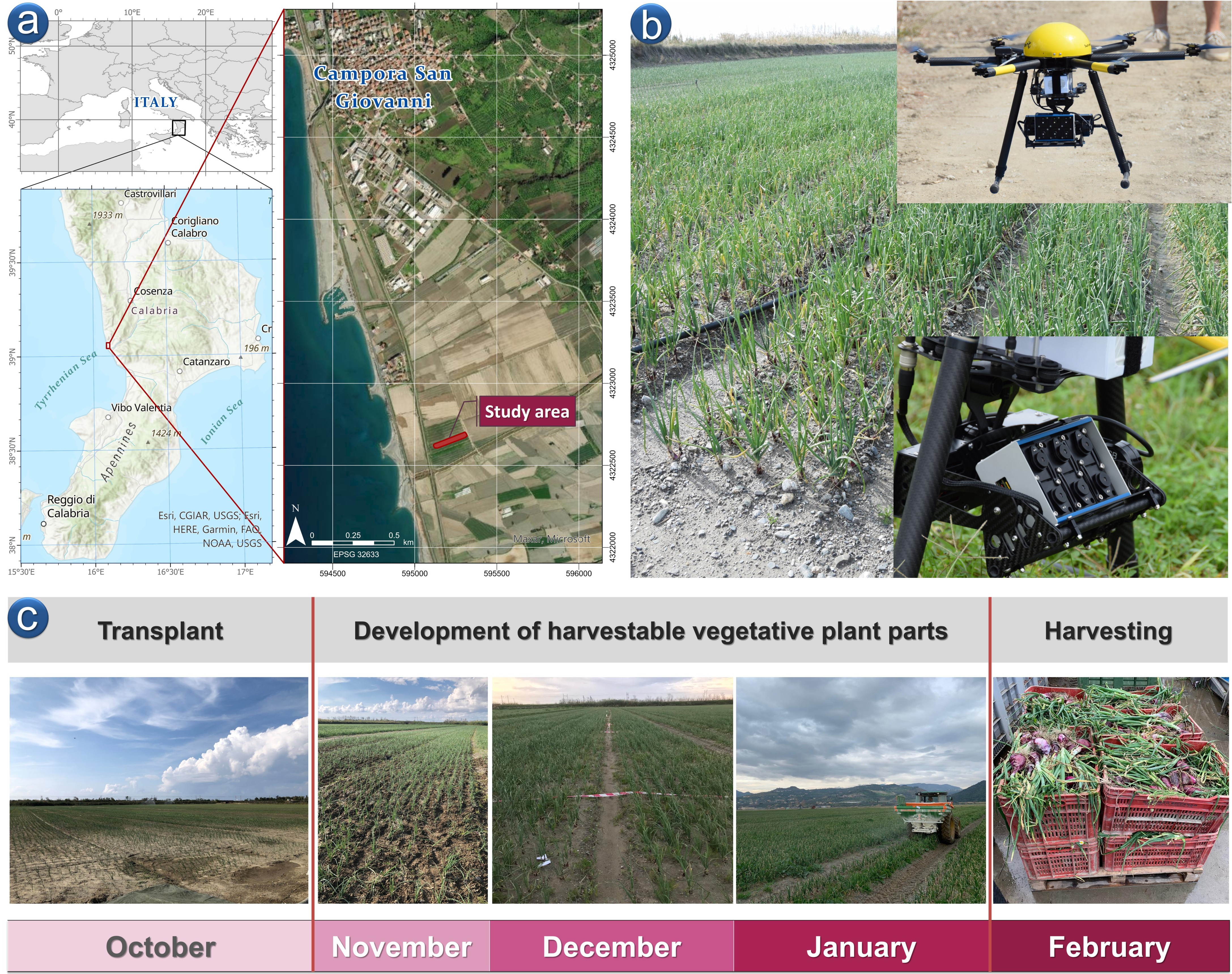
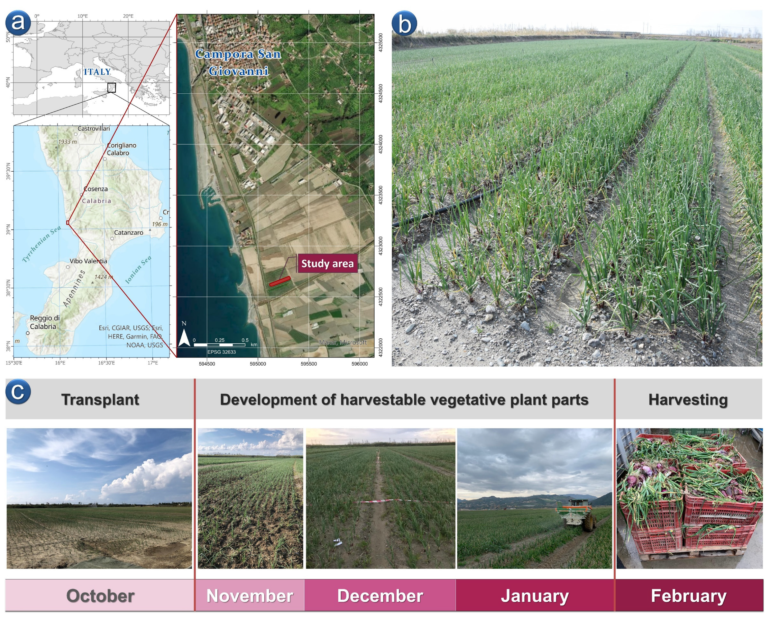
The workflow showed in Figure 1 summarizes the methodology adopted in the different phases: (a) soil sampling and analysis, (b) experimental sample scheme of N fertilization and harvesting, (c) UAV surveys and pre-processing, (d) image data pre-processing and (e) image segmentation and classification aimed at the production of vigor maps.

2.1. Study Site

The onion field is located in Campora S. Giovanni, in the municipality of Amantea (Cosenza, southern Italy, 39°02′52″ N, 16°06′03″ E, 6 m a.s.l) (Figure 2a). The farm is part of a consortium whose cultivated area is over 700 hectares [31], involving more than 100 farms and giving a total production of 21Mt for an economic value close to 11 million euro [32]. The onion represents a significant crop production in the Calabria region [6]. The success of this product on the national and international markets relies on its unique intrinsic characteristics, such as the organoleptic properties [33] and the presence of nutraceutical compounds that make the Tropea red onion a “functional food” [34,35]. These characteristics allowed obtaining the brand European Protected Geographical Indication “Cipolla Rossa di Tropea Calabria IGP”.

The experimental site’s soil is a Typic Xeropsamments [36], and the fields are flat (slope ≤ 3%). The main soil properties, determined at the beginning of the experiment by soil sampling (before the start of the cultivation cycle, at the end of September) and referring to the 0–20 cm top layer (Ap horizon), were as follows: pH 7.51 (in water), electrical conductivity (EC1:2) 431.11 µS cm⁻¹, sandy texture (USDA), soil organic matter (SOM) 1.49 %, total organic carbon (TOC) 14.9 g kg⁻¹, total nitrogen (TN) 0.50 %, total inorganic carbon (TIC, CaCO₃-C) 35 g kg⁻¹, available P (Olsen) 36.18 mg kg⁻¹, nitrate (NO₃⁻-N) 41.93 mg kg⁻¹, ammonium (NH₄⁺-N) 10.27 mg kg⁻¹.

The study site covers a surface of 0.63 hectares and is less than 300 m from the sea coastline. The field (Figure 2b) is crossed by two paths, 3-m wide, where the agricultural vehicles pass while executing phytosanitary treatments and fertilization.

The plants are placed at 15 × 15 cm from each other on a 3-m-wide soil bed. Any weeds on the soil bed were removed manually. The transplant was completed at the beginning of October (autumn), while the harvest was in early February (mid-winter) (Figure 2c).

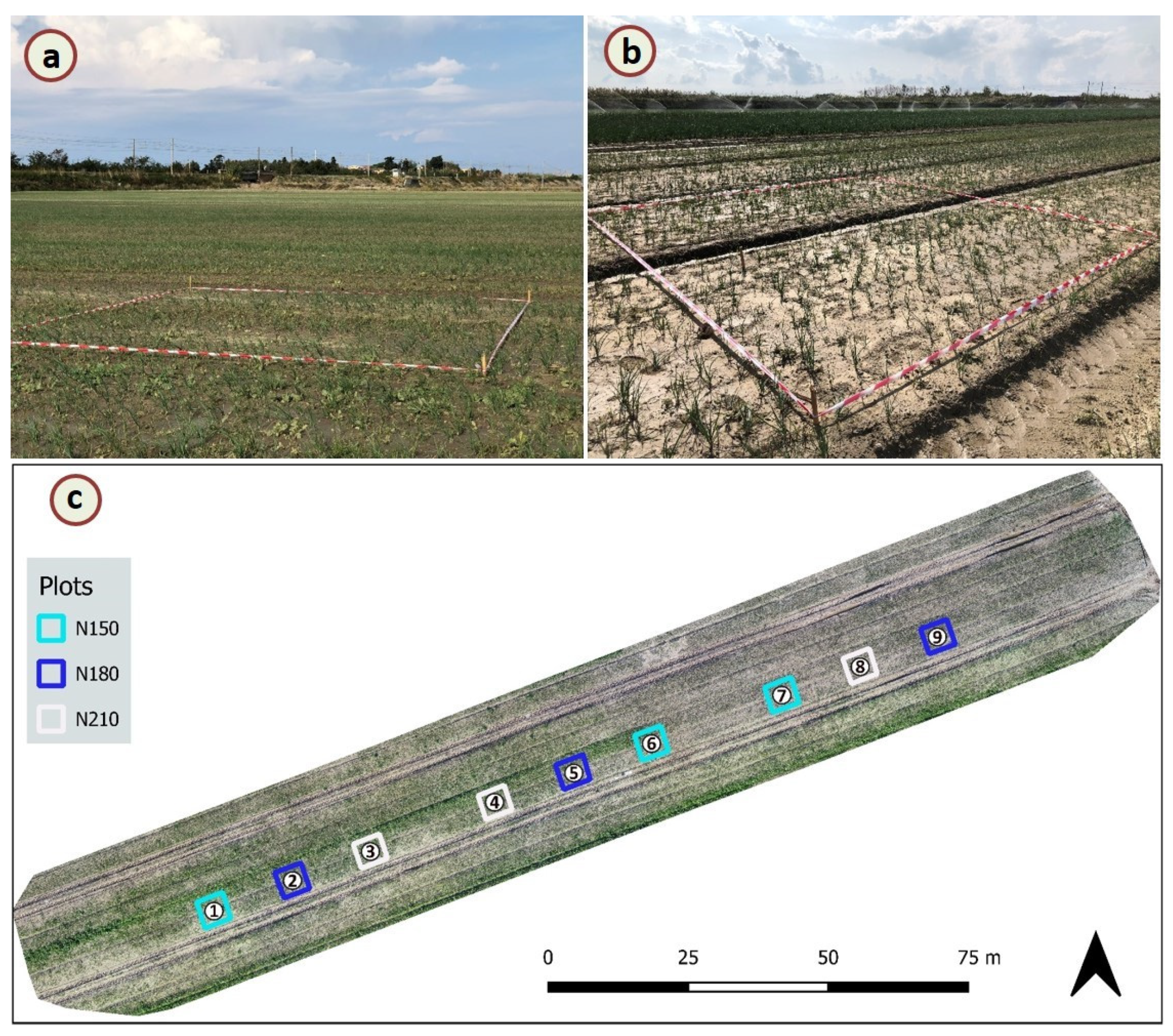
2.2. Experimental Design and Crop Management

The experimental setup consisted of field plots (5 m × 5 m each), delimited using steel stakes placed at the corners of each plot (Figure 3a,b). They were arranged in a randomized complete block design (RCBD), with three replications, in order to compare three different levels of N fertilization (Figure 3c): N150 (150 kg N ha⁻¹), the typical N dose applied by the local farmers; N180 (180 kg N ha⁻¹); and N210 (210 kg N ha⁻¹).

According to traditional practices, basal fertilization was carried out before onion transplanting with 400 kg ha⁻¹ of 20N-10P₂O₅-10K₂O chemical fertilizer, involving all field plots. At the same time, N was provided with two top-dressing fertilizations during the cropping season, with different doses according to the treatments with ammonium nitrate (34% N) and ammonium sulfate (20.6% N).

Finally, at the end of the growing season, onions from each experimental plot were manually harvested, the relative fresh yield was determined, and soil sampling was carried out.

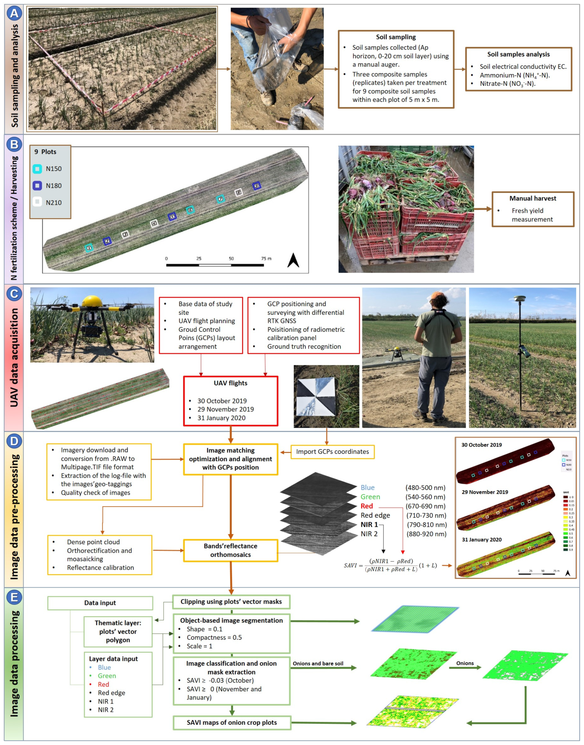
2.3. Soil Sampling and Statistical Analysis of Soil Parameters

Soil sampling was carried out within each plot in early February at the harvest. Soil samples were collected (Ap horizon, 0–20 cm soil layer) using a manual auger from the middle of each plant’s inter-row space to minimize any border and plant effect and then thoroughly mixed to form a unique composite sample representative of the replicate. Three composite samples (replicates) were taken per each treatment, thereby obtaining nine composite soil samples. In the laboratory, each sample was split into two aliquots: a representative amount of moist field soil (100 g) was promptly (within 24 h) processed for NH₄⁺-N and NO₃⁻-N analysis, whereas the remaining aliquot (100 g) was air-dried, sieved to pass through a 2-mm sieve, and then stored at room temperature before electrical conductivity (EC) determination. Soil EC was measured in 2-mm-sieved and air-dried soil at 25 °C in a 1:2 (w/v) soil-to-water ratio mixture (EC_1:2 at 25 °C). The soil NH₄⁺-N and NO₃⁻-N concentration in 2 M KCl soil extracts (1:10, w/v) was determined colorimetrically by the Berthelot reaction and Griess–Ilosvay method, respectively, by using a flow injection analysis system (FIAS 400 PerkinElmer, Inc., Richmond, CT, USA) equipped with an AS90 autosampler (PerkinElmer) and linked to a UV/Vis spectrophotometer Lambda 25 (PerkinElmer).

Soil chemical data are reported as mean values (n = 3) and were expressed on a dry-weight (DW) basis (105 °C, 24 h). Data were first tested for deviation from normality (Kolmogorov–Smirnov test) and homogeneity of within-group variances (Levene’s test). A one-way analysis of variance (ANOVA) was performed to highlight the effect of soil treatments on tested soil chemical variables and onion yield. Tukey’s HSD test at p < 0.05 was used for multiple pairwise comparisons of treatment means. Statistical analyzes were performed by using R software [37].

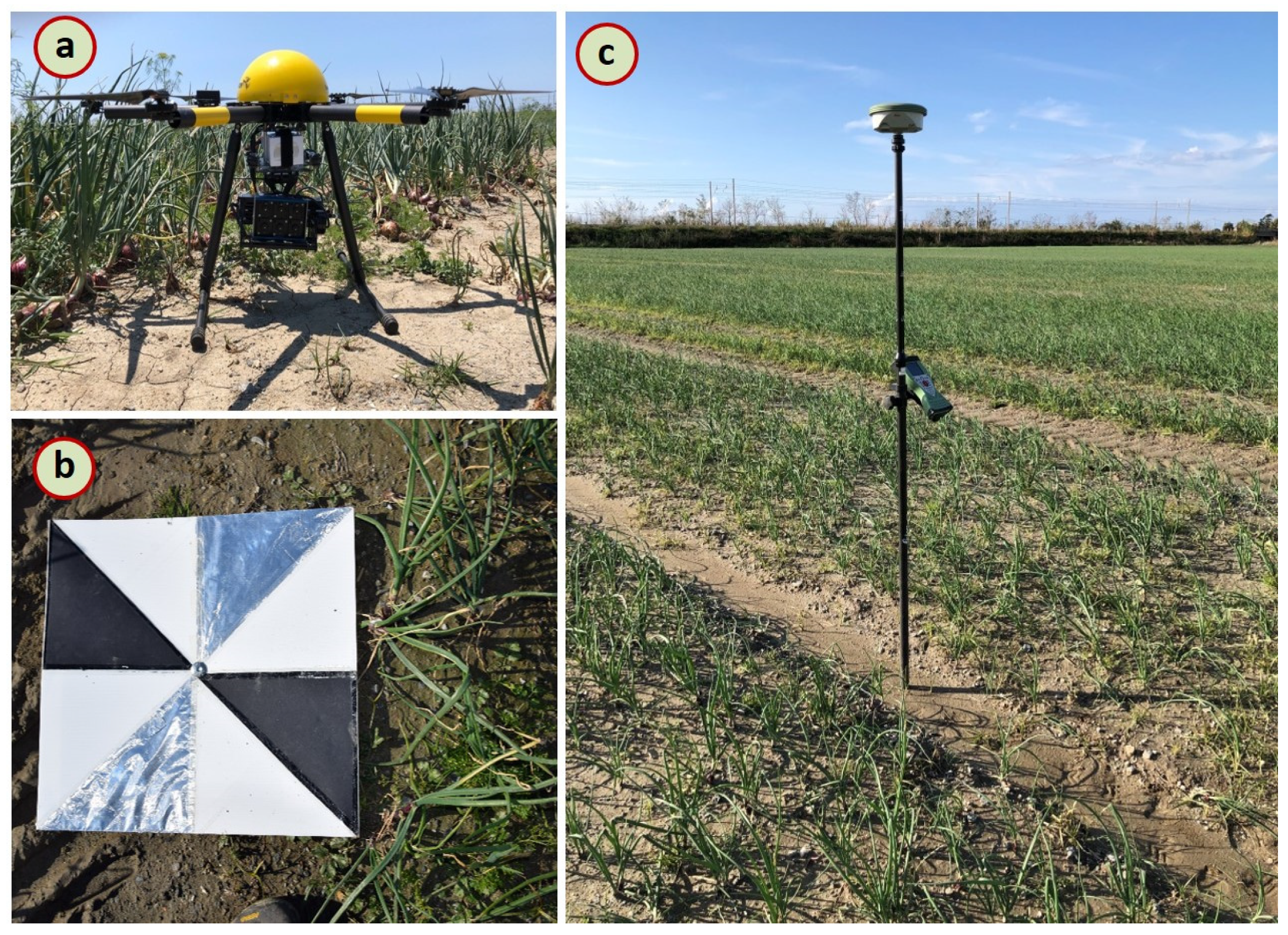
2.4. UAV and Image Data Acquisition

The UAV surveys were carried out between the early middle (October) and the end of the cultivation cycle (early February). During this period, the UAV flights were performed three times; the first on 30 October 2019, the second on 29 November 2019, and the last on 31 January 2020 (

Table 1. Tetracam µ-MCA06 snap sensor and flight characteristics.

Geometry of Lens	Sensors	Bands	Spectral Wavebands (nm)	Central Band Wavelength [nm]	Bandwidth [nm]
Focal length (fixed lens) 9.6 mm Dimension 6.66mm × 5.32mm 1.3 Megapixel CMOS 4:3 format 1280 × 1024 pixels Pixel size 4.8 microns Angle of View (W × H) 38.26° × 30.97°	Master (0)	Near-infrared (NIR1)	790–810	800	10
	1	Blue	480–500	490	10
	2	Green	540–560	550	10
	3	Red	670–690	680	10
	4	Red edge	710–730	720	10
	5	Near-infrared (NIR2)	880–920	900	20
	Date	Take-off time [UTC+1]	Total duration [min]	Flight height [a.g.l.]	Speed [m s−1]	Sidelap and Overlap [%]
	2019/10/30	11:30 am	20	30 m	2.5	80
	2019/11/29	12:00 am	19	30 m	2.5	80
	2020/01/31	10:30 am	19	30 m	2.5	80

), in correspondence with the following onion growth stages: leaf development, 109 BBCH-scale phase (30 October 2019); 30% of bulb development, 403 BBCH-scale phase (29 November 2019); complete bulb growth, 409 BBCH-scale phase (31 January 2020) [38].

The first two dates correspond to the phase of the crop cycle in which there is the full development of harvestable vegetative plant parts. On the last date of the survey, at the end of January, the harvest is close.

Surveys were carried out at 30 m of flight height using a multirotor UAV (Multirotor G4 Surveying Robot—Service Drone GmbH) (Figure 4a). Multirotor G4 is equipped with six high-efficiency brushless electric motors, gimbals, and flight control with a dual 32-bit processor. The UAV was equipped with an MS camera Tetracam µ-MCA06 snap (Tetracam Inc.—Chatsworth, GA, USA). This camera has six different 1.3-megapixel CMOS sensors (4:3 format, 1280 × 1024 pixels) and an interchangeable bandpass filter housed in the unit called “master,” as it can synchronize the unit called “slave” (Table 1).

In this way, each sensor shoots simultaneously, and all images of the bands are synchronized. These bands are blue (480–500 nm), green (540–560 nm), red (670–690 nm), red edge (710–730 nm), NIR1 (“master” channel, 790–810 nm), and NIR2 (880–920 nm). The MS camera was equipped with its global navigation satellite system (GNSS), the FirePoint 100 GPS. All flights were conducted at an altitude of 30 m a.g.l. under constant scene illumination and cloud-free conditions.

The ground sample distance (GSD) was 1.5 cm. Ground control points (GCPs) were placed in the field to obtain a high-quality geolocated output. GCPs were made using 50 cm × 50 cm black and white polypropylene panels (Figure 4b). Each GCP’s position coordinate (WGS 84/ETRF 1989 UTM 33N) was georeferenced using a Leica GS12 RTK GNSS (Figure 4c) with planimetric and altimetric accuracy of ±2.5 cm and ±5 cm, respectively.

2.5. Image Data Pre-Processing

To perform the conversion from digital number (DN) to reflectance value, the reflectance of grey on the field calibration target (50 cm × 50 cm polypropylene panel) was measured through the spectroradiometer Apogee Ps-300. All the images were extracted from the camera and subsequently converted from the *.RAW format to 10-bit TIFF format through PixelWrench II (version 1.2.4, Tetracam Inc—Chatsworth, GA, USA). Images were then aligned, stacked, and radiometrically corrected using Pix4D mapper Pro (version 4.3—Pix4D SA, Prilly, Switzerland). Reflectance values measured on a grey calibration panel placed in the field were extracted in correspondence with each central band and used to calibrate images. Finally, reflectance orthomosaics were generated for each band and stacked into a single multiband orthomosaic for each of the six bands (blue, green, red, red edge, NIR1, and NIR2).

2.6. Image Data Processing: Segmentation, Classification, and SAVI Maps

A GEOBIA process was developed on the orthomosaics resulting from UAV image processing to discriminate onion crops from the soil. Image data processing was performed using the eCognition Developer 10 software (Trimble GeoSpatial, Munich, Germany).

Considering the characteristics of the field that includes portions of soil well visible between individual plants and in the paths of the passage of agricultural vehicles, classification was performed to separate onions and soil. The classification was developed by exploiting only the vegetation’s spectral response in the different bands, as in Modica et al. [39] and Messina et al. [6]. Firstly, the procedure of segmentation of the image was performed. Segmentation is a fundamental pre-requisite for classification/feature extraction [40] as the resulting segments (i.e., image objects containing soil or vegetation/onion plants in our case) form the basis for the subsequent classification step [41]. Furthermore, object-based approaches provide accurate results when using very-high-resolution imagery [42,43]. This step foresees the image segmentation into separate, non-overlapping regions [44], subsequently extracted in the form of vectorial objects. We implemented the segmentation step on the Multiresolution Segmentation (MRS) algorithm [45], which works by identifying single-pixel objects and merging them with closer objects following the relative homogeneity criterion [46]. This criterion depends on combining the original image’s spectral and shape properties and new objects generated by the merging process. Therefore, two parameters regulated homogeneity criteria: shape and compactness. The shape parameter is set by a weight attributed to the shape of objects with respect to color. The shape parameter value can range from 0 to 0.9. Color homogeneity depends on the standard deviation of spectral colors. When choosing the parameter’s value, the higher the selected value, the greater the influence of the shape with respect to the color during segmentation and vice versa [47]. Compactness is the second parameter; the importance of the shape with respect to the smoothness depends on it. It derives from the product of width and length calculated on numbers of pixels [48].

In addition to the shape and compactness parameters, the scale parameter determines the final size and dimension of the objects deriving from segmentation [40,45,46,49]. So smaller values of the scale parameter produce smaller objects and vice versa with higher values. Scale parameter indirectly defines the maximum allowed heterogeneity for the resulting image objects. In addition to the parameters indicated so far, several weights can be attributed to the input data (in this case, band layers). These parameters were chosen to perform segmentation: 0.1 for shape, 0.5 for compactness, 1 for scale parameter, applied to bands/layers provided by Tetracam µ-MCA06: blue, green, red, red edge, NIR1, and NIR2. Before choosing these parameters, some trial-and-error tests were performed, based on visual interpretation, by testing attributing different values to the segmentation parameters until the segmentation considered better was obtained. Specifically, the segmentation assumed as the most helpful with the research objectives was the one generating objects capable of isolating individual plants.

For monitoring onion crops in UAV imagery, the soil-adjusted vegetation index (SAVI) was chosen to analyze the vegetative vigor [4,6,50,51]. SAVI was developed by Huete [52] to minimize the effects of soil background on the vegetation signal by using a constant soil adjustment factor, L, which can take a value between 0 and 1 depending on the level of vegetation cover inserted in the normalized difference vegetation index (NDVI) formula, according to this formula Equation (1):

$$SAVI=\frac{\left(\rho NIR-\rho Red\right)}{\left(\rho NIR+\rho Red+L\right)}\left(1+L\right)$$

(1)

where $\rho$ is the reflectance at the given wavelength.

The SAVI, being one of the soil-corrected vegetation indices [53], allows further reduction of the background contribution reflectance by making it easier to detect onions, discriminating them from background soil as shown in [6]. Initially, the SAVI was calculated on the images of the entire field and histograms were used for a preliminary analysis over the months investigated. Then, descriptive statistics were used to analyze SAVI values referring only to onions identified within the single plots. For this reason, after the segmentation step, the classification of onions and bare soil was performed. The onion crops were classified by exploiting a SAVI (L = 1) threshold value ≥ −0.03 in the October image and a SAVI (L = 0.5) threshold value > 0 in November and January images.

These threshold values were chosen as a result of some trial-and-error tests. It was judged better based on visual interpretation considering its ability to detect onions, following the same methodology shown in Modica et al. [39]. The data obtained concerning only the class “onions” was used to create a mask to be applied to each of the three SAVI maps derived from UAV images.

A geometrical mask of 0.3 m × 5 m was used to exclude any weeds from each plot in the space between the soil beds. The masks were applied to the UAV images to obtain only parts of SAVI maps concerning the onion crop.

3. Results and Discussion

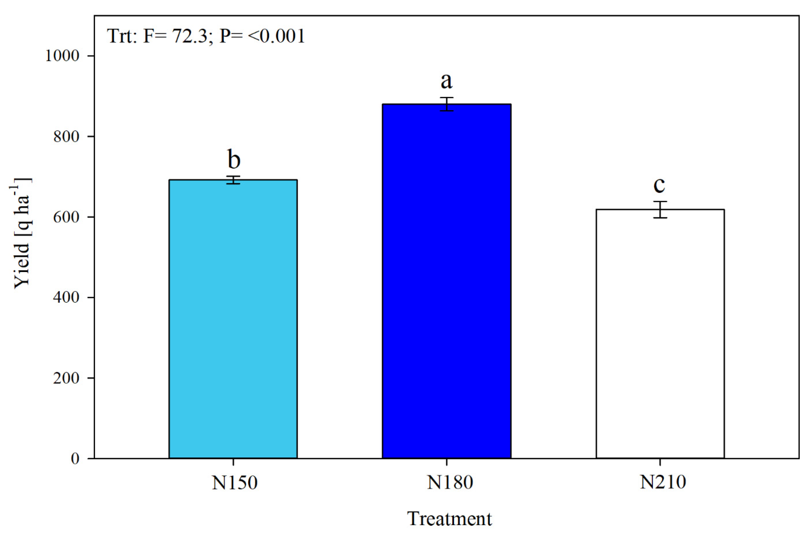
3.1. Chemical Soil Parameters and Fresh Onion Yield

N fertilization managements significantly affected (p < 0.05) all soil chemical properties investigated (

Table 2. Effects of the three different N fertilization managements (N150 (150 kg N ha⁻¹), N180 (180 kg N ha⁻¹) and N210 (210 kg N ha⁻¹)) on soil electrical conductivity (EC), ammonium-N (NH₄⁺-N) and nitrate-N (NO₃⁻-N) in the onion crop plots. Data presented are means (n = 3). At the bottom, one-way ANOVA results are presented as F- and p-values. Different letters indicate significant differences among treatments (Tukey’s HSD test, p < 0.05).

	EC [µS cm−1]	NH4+-N [mg kg−1]	NO3−-N [mg kg−1]
N150	286.8c	7.3c	38.8c
N180	394.5b	17.1b	58.4b
N210	1002.8a	37.8a	168.2a
One-way ANOVA
F-value	680.5	238.0	51.0
p-value	<0.001	<0.001	<0.001

). In particular, the increase of N dose applied determined a consistent raise of soil EC, NH₄⁺-N and NO₃⁻-N concentrations.

Regarding soil EC, at the lowest N dose applied (N150), the value recorded was equal to 286.8 µS cm⁻¹, while greater N doses (N180 and N210) showed higher values of +38% and +250%, respectively, for N180 and N210. Soil EC determination represents an indirect measure of soil soluble salts concentration in its liquid phase. EC expresses the availability of soluble species present in the soil as an indicator of soil salinity status, including the chemical elements essential for the plant’s mineral nutrition and the saline compounds that are potentially harmful to crops, especially for the susceptibility to salinity. This parameter’s value can depend on several factors related to the soil’s intrinsic properties and management. In agricultural soils, factors such as the climatic trend, irrigation water quality and fertilization could significantly affect soluble salts concentration in the soil [54,55]. Among vegetable crops, the onion is a species that is highly susceptible to salinity [21,56]. For this species, a salt tolerance threshold equal to 1.2 dS m⁻¹ was estimated [57,58,59,60].

Soil NH₄⁺-N and NO₃⁻-N concentrations observed in N150 treatment were the lowest retrieved and equal to 7.3 and 38.8 mg kg⁻¹, respectively. Increased N dose distribution augmented both mineral N forms (NH₄⁺-N and NO₃⁻-N) by +133% and +51% for N180 and by +414% and +334% for N210. Mineral N fertilization strategy is one of the main factors that sustain onion growth and production [61,62]. Indeed, N had a critical role during photosynthesis, is fundamental to form chlorophyll, controls numerous processes of plant metabolism, and is also an indispensable part of co-enzymes and proteins. Therefore, N has been reported as the most critical yield-limiting nutrient for many crops [20]. In any case, the fertilization strategy should be carefully thought through. In fact, excesses of N can determine accelerated growth, delay of bulb maturity, increased susceptibility to pests and diseases, reduced dry-matter content, limited shelf life, and result in low onion yield and quality [63,64,65]. Moreover, a prudent strategy for N fertilization management is required in order to avoid N losses in the environment that can cause air (N gaseous emission) and water (N leaching) pollution and ensure crop production sustainability. Therefore, soil availability for the crop could meet crop requirements in order to achieve a higher fertilizer utilization efficiency, avoid pollution and, as a result, reduce costs and obtain the highest crop profit.

Fresh onion yield was significantly affected by the fertilization management applied (p < 0.05) (Figure 5). The highest yield was registered for N180 treatments, equal to 890 q ha⁻¹, while lower productions were observed for N150, equivalent to 692 q ha⁻¹ (−21%), and N210 with 619 q ha⁻¹ (−30%). The yield registered in the current experiment is near the productivity observed in other studies carried out within and abroad of Europe [66,67,68]. In particular, concerning fertilization management, as in our experiment, the highest yield with similar production was also obtained with a dose of 180 kg N ha⁻¹ by Díaz-Pérez et al. [69], Rodrigues et al. [70], and Gonçalves et al. [71].

As argued by García et al. [72] and Machado and Serralheiro [73], the increase of the level of salts in the soil solution can affect water and nutrient absorption, resulting in a metabolic imbalance that can lead to the reduction of plant growth and production, as observed in the current research and also reported by Medeiros Pessoa et al. [74] and Lima and Bull [75]. Indeed, soil salinity stress can determine a stunted development of plant foliage, with a reduction of leaves per plant and leaf height necessary to achieve a high production [76,77,78]. Shannon and Grieve [79] observed that due to salinity stress, leaves change their color from brilliant green to dull blue-green caused by inhibition in the synthesis of chlorophyll, and leaf tips express burn symptoms with a reduction of photosynthesis. Among plant growth phases, in particular, bulb growth is the period most sensitive to water and salinity stress, according to Kadayifci et al. [80] and Sta-Baba et al. [78], with negative consequences on both fresh weight and product quality. Moreover, beyond its direct effect on plant physiology, salinity weakening the plant can increase susceptibility to the diseases [81,82]. Among product quality indices, salinity negatively affects the mean bulb morphology, weight, diameter, and consistency [82,83].

Onion yield is strictly linked to N fertilization and is directly proportional to the amount of N supplied to the crop. However, onion growth is stimulated by N fertilization up to a specific limit, beyond which no benefit is observed for the crop [65,84,85]. Among the studies regarding onion N fertilization, Jilani et al. [86] observed the highest onion yield with 200 kg N ha⁻¹, while other studies [65,68,87,88,89,90] reported a range between 100 and 180 kg N ha⁻¹ to achieve the best yield performance. According to several authors, the increment of yield related to N fertilization augments is attributable to an increased plant height, leaf area, bulk weight, and diameter [65,89,90]. Moreover, it was also reported that optimal N fertilization could increase vitamin C concentration in bulbs [90]. Furthermore, it was observed that higher than optimal N fertilizer doses reduce the crop productivity level due to the appearance of phytotoxicity phenomena on plants [91,92] and plant susceptibility to diseases [93,94], also decreasing the commercial production [69,95]. However, differences in optimal N dose could be ascribable to the different varieties, environmental conditions, soil characteristics, and management. Even so, our results agree with the trend observed from the other studies, as argued above, highlighting a positive yield trend from N150 to N180 and then decrease as the administered dose increases (N210). This evidence suggests that increasing the N dose up to 180 kg N ha⁻¹ produces increasing benefits for plant metabolism and growth, thus stimulating crop yield of Tropea red onion; increased N dose beyond this threshold harmed production, triggering a vicious circle wherein the progressive increase of N application determined a reduction of nutrient assimilation from the crop due to the progressive increase of soil EC, and thus soil salinity, to which onion is particularly susceptible.

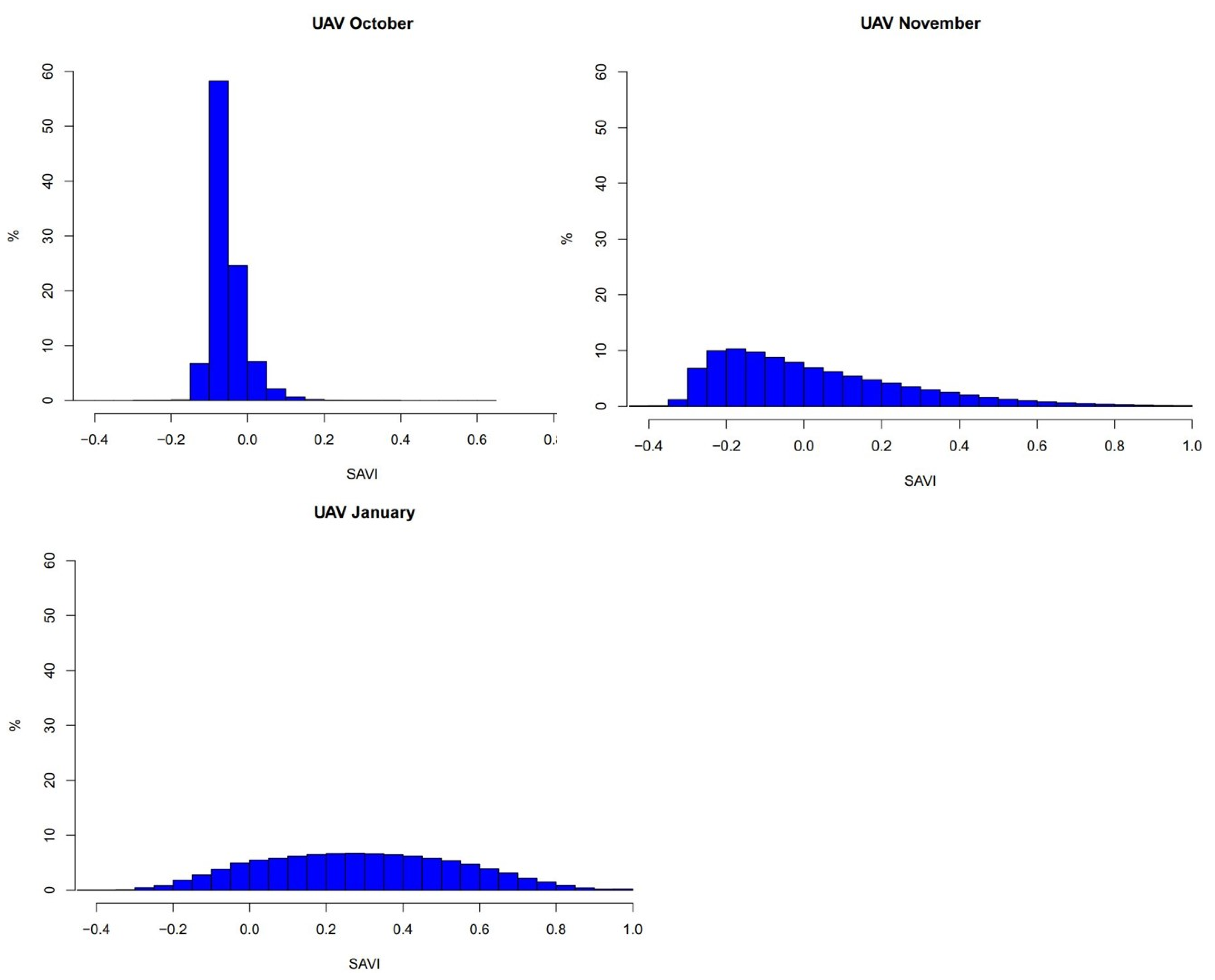
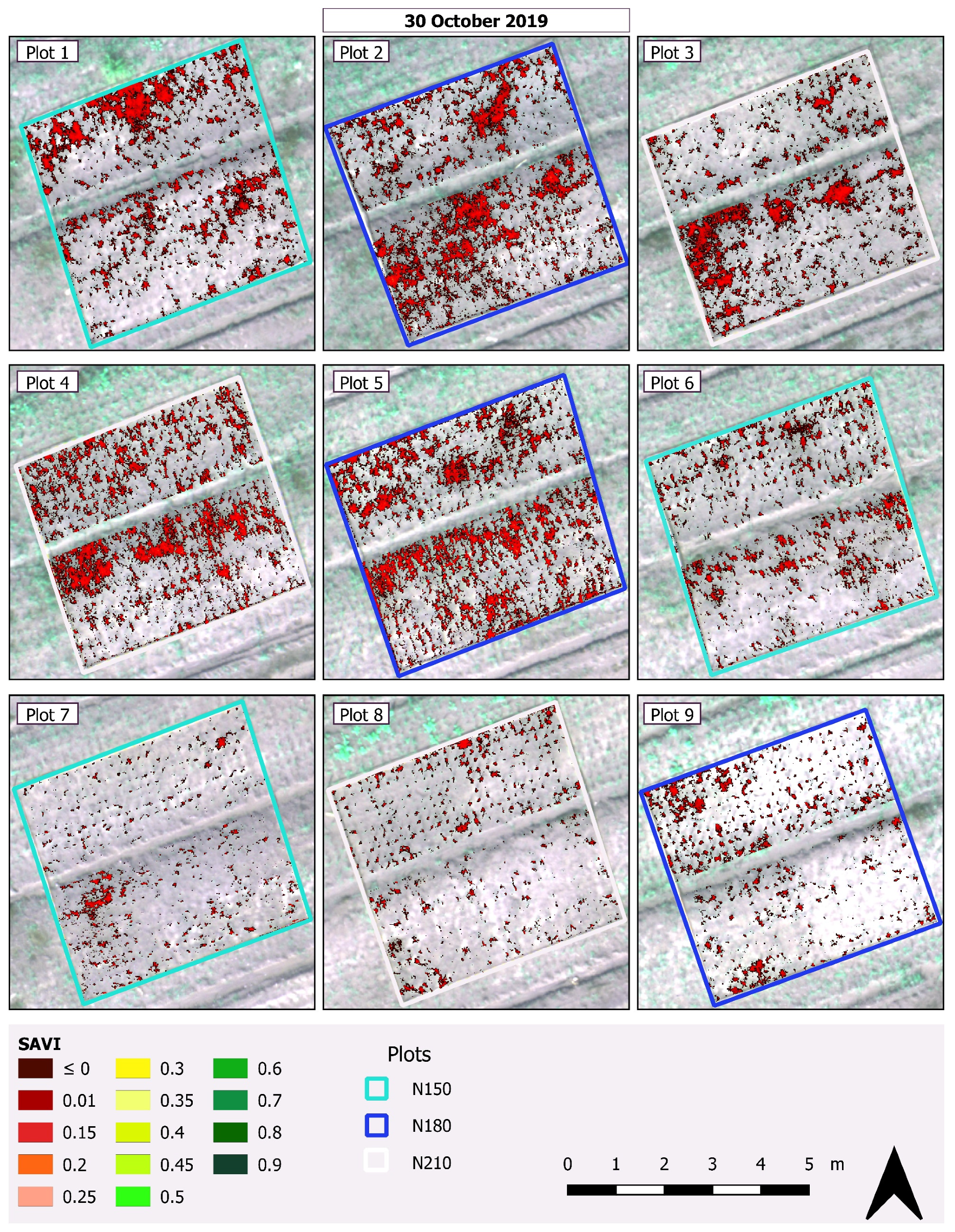
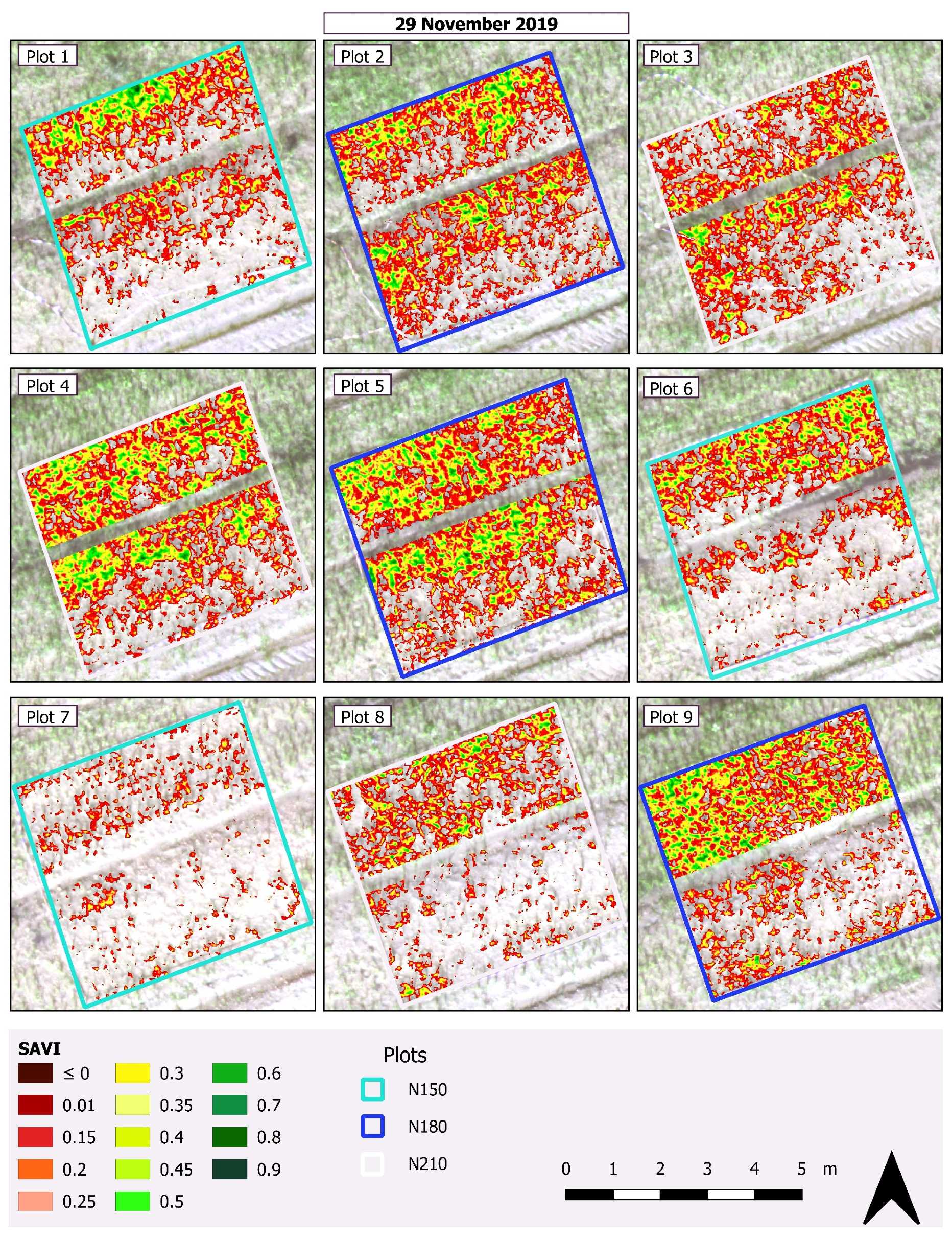
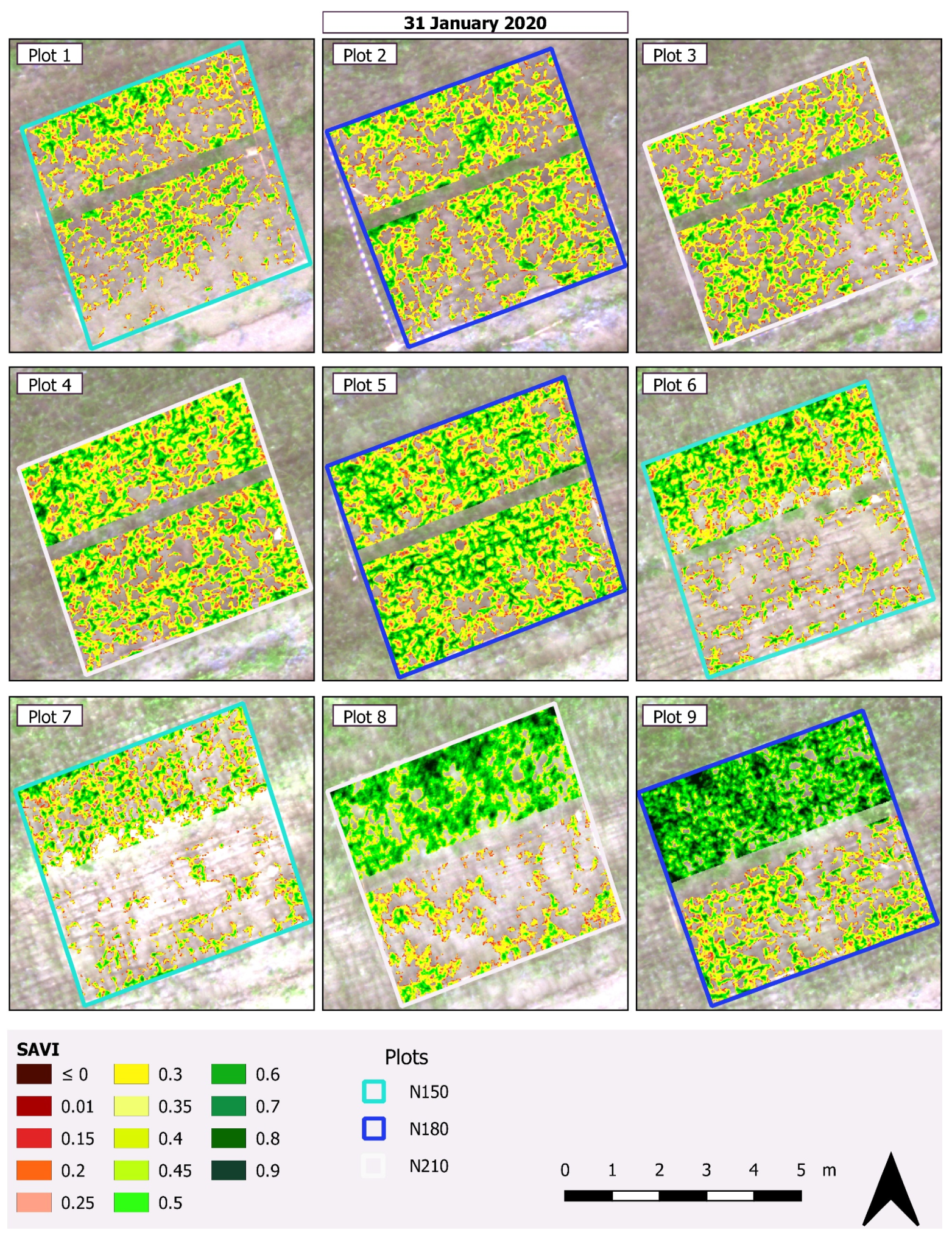
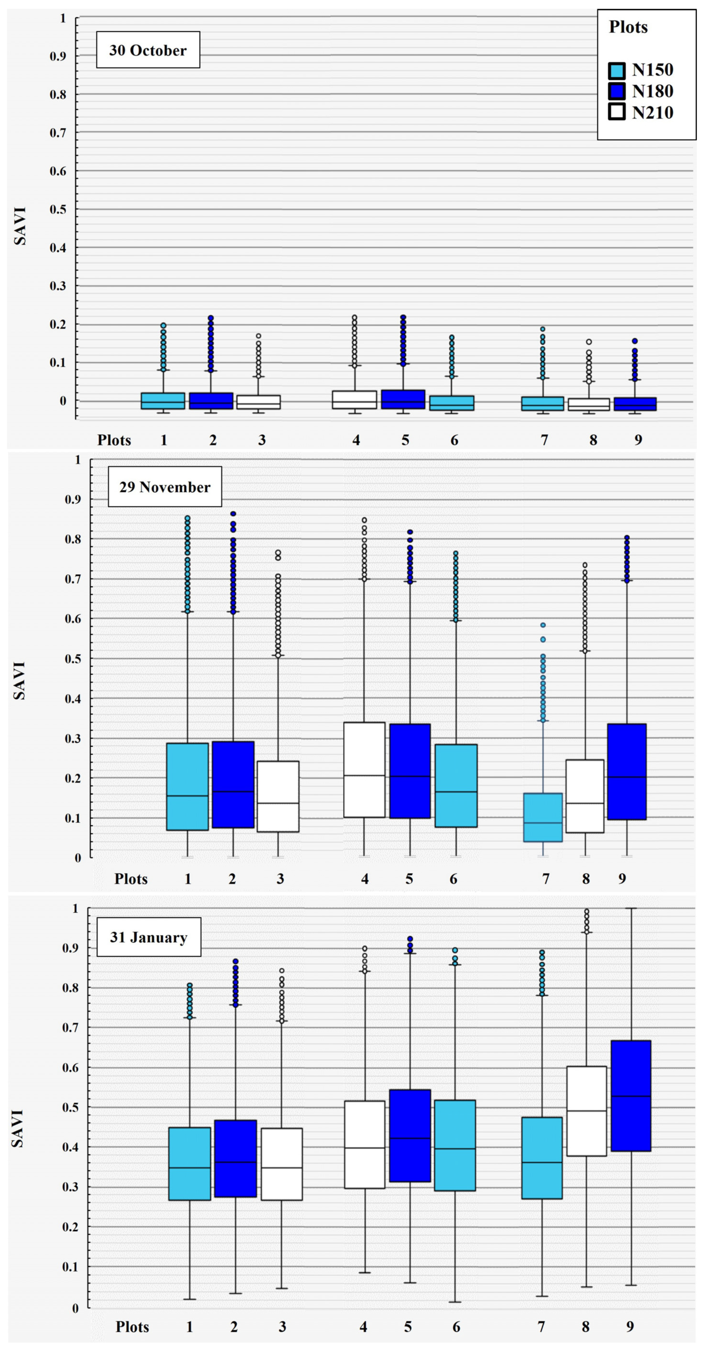
3.2. Soil-Adjusted Vegetation Index Maps

SAVI vigor maps of the entire field are shown in Figure 6. Considering the image of October, at the beginning of the transplant, SAVI’s values are shallow, ranging from 0 to 0.15. This is mainly due to the soil’s predominant presence, with a value of 0, compared to the still tiny plants with thin leaves, especially in the early stages of growth [26].

In November, SAVI’s value ranged from values below and equal to 0 up to 0.7. The crop’s presence is beginning to become evident, and its coverage relative to the soil is more significant than in October. The paths followed by agricultural vehicles are also easily identifiable.

Lastly, in January, SAVI’s value range is between 0.15 and 0.9. The lowest values, close to 0 (black in the maps), are primarily found in agricultural vehicles’ side paths. The medium–high values, between 0.4 and 0.9, belong to the crop’s vegetation, which is prevalent concerning the soil, also considering the upcoming harvest.

The histograms reported in Figure 7 show the frequency distribution of SAVI values as a percentage of each imagery’s total values. In October, more distribution of values is at −0.1. A more homogeneous distribution in the range between −0.2 and 0 can be observed in November. In January, a large part of the values’ distribution is above 0, between 0.1 and 0.5. These SAVI maps were inherent to the whole field.

To analyze only the onion, SAVI computed on the onion crop within the nine plots was considered. In particular, other maps were generated using the masks produced on eCognition, following the same methodology adopted in Messina et al. [6]. The masks obtained by exporting a vector file containing only the class “onions” were applied to the UAV images with the aim to focus only onions present within the plots subjected to the different fertilization treatments. Consequently, parts of the scene of the image identified as bare soil were excluded from the map (Figure 8, Figure 9 and Figure 10).

In Figure 8, showing SAVI calculated on the onions mask in the October image, what is shown in Figure 6 is confirmed, as the crop takes on values between 0 and 0.15.

The SAVI mean in the single plots, as can be seen in

Table 3. Basic statistics of the soil-adjusted vegetation index (SAVI’s mean and standard deviation), onion cover (expressed in m²) considering only the nine plots (5 m × 5 m) chosen to compare three different levels of nitrogen fertilization (N150 (150 kg N ha⁻¹), N180 (180 kg N ha⁻¹) and N210 (210 kg N ha⁻¹)). The last column on the right shows the yield obtained.

30 October				29 November				31 January				Onion Harvested [q ha−1]
Plot ID	SAVI		Onion Cover [m2]	Plot ID	SAVI		Onion Cover [m2]	Plot ID	SAVI		Onion Cover [m2]
	Mean	St. Dev			Mean	St. Dev			Mean	St. Dev
(1) N150	0.006	0.005	5.79	(1) N150	0.19	0.030	9.55	(1) N150	0.36	0.055	9.65	692
(2) N180	0.005	0.005	6.86	(2) N180	0.20	0.025	13.24	(2) N180	0.40	0.050	12.68	890
(3) N210	0.001	0.004	4.89	(3) N210	0.17	0.026	11.05	(3) N210	0.36	0.051	11.91	580
(4) N210	0.010	0.006	6.46	(4) N210	0.23	0.027	13.77	(4) N210	0.41	0.036	17.01	628
(5) N180	0.011	0.006	7.49	(5) N180	0.23	0.023	15.35	(5) N180	0.43	0.040	18.60	860
(6) N150	0.001	0.006	3.75	(6) N150	0.19	0.029	8.70	(6) N150	0.41	0.062	11.05	676
(7) N150	0.001	0.005	1.77	(7) N150	0.11	0.035	3.07	(7) N150	0.38	0.052	8.40	708
(8) N210	0.001	0.006	2.11	(8) N210	0.17	0.030	7.41	(8) N210	0.49	0.090	12.67	648
(9) N180	0.001	0.006	2.76	(9) N180	0.23	0.034	12.0	(9) N180	0.53	0.060	16.01	868

SAVI: soil-adjusted vegetation index; St. Dev: standard deviation. The grey color is the best results obtained applying the N180 dose.

, is close to 0. This can be explained by taking it into account during the segmentation phase. The classification algorithm was not always able to correctly separate the vegetation from the soil in the background, as shown in Jeong et al. [26] and Messina et al. [6]. For this reason, during the onion classification phase, pixels with a value equal to or very close to 0 were selected, including both vegetation, consisting of thin leaves, and portions of the underlying soil.

This affected the average SAVI value of the nine plots in the October image. This is observable in the boxplots’ trend in Figure 11, in which numerous outliers represent the crop’s SAVI values. The SAVI mean is similar in all the plots, considering that no differentiated fertilizer treatment has been performed yet.

In Figure 9, showing SAVI calculated on onions mask in November image, the crop takes on values between 0.15 and 0.6. The SAVI mean in the single plots, as can be seen in Table 3, is higher than that seen in October, with values between 0.11 and 0.23. In particular, the lowest value was found in plot 7 (N150), while the higher value belongs to plots 4 (N210), 5 and 9 (N180). Furthermore, it is possible to notice also, as in plots 2, 5, and 9 (N180), that the average of the SAVI is always equal or superior to 0.20. Small portions of the crop where there are higher SAVI values (progressively colored from light green to dark green in Figure 9), between 0.5 and 0.8 (except for plot 7 (N150)), are also highlighted by the outliers in the boxplots in Figure 11.

The SAVI calculated on the onions mask in the January image, the crop, close to harvest, takes on values between 0.3 and 0.9, as shown in Figure 10 (between yellow and dark green), confirming a progressive increase compared to November. The SAVI mean in the single plots, shown in Table 3, ranges from 0.36 to 0.53. In detail, the lowest values, 0.36 and 0.38, were found in plots 1 (N150), 3 (N210) and 7 (N150). On the other hand, the higher value belongs to plots 8 (N210) and 9 (N180) with SAVI means equal to 0.49 and 0.53, respectively, made evident by looking at the predominant dark green in Figure 10. In particular, these very high SAVI values, starting at 0.75 and exceeding 0.9, can be inferred from the outliers and the trend of the boxplots in Figure 11.

3.3. Relationship between Nitrogen Fertilization, Onion Yield, and SAVI Mapschemical Parameters and Fresh Onion Yield

The information retrieved from the analysis of soil properties (EC, NH₄⁺-N, and NO₃⁻-N), yield performance, and mean SAVI index data from each field plot showed significant relationships between the different indicators investigated. In particular, the observation of the soil analysis related to the soil EC and the concentration of NH₄⁺-N and NO₃⁻-N confirmed that the increasing levels were going from plots N150 to plots N210, while the SAVI index, interpreting the effect from the interaction between soil properties and onion plants, was positively correlated with yields, as can be observed in Table 3.

Along the cropping cycle, in the initial phase of the crop cycle, in October (leaf development, 109 BBCH phase), before the differentiation of the fertilizer treatment, no significant differences in vegetative vigor were observed in the different plots. This is shown by a similar mean SAVI value in plots with different N fertilizer doses: 0.002 (N150), 0.005 (N180), and 0.004 (N210). In the following months, the differences became more evident (November, 30% of bulb development, 403 BBCH phase; January, complete bulb growth, 409 BBCH phase). In November, the mean SAVI value in plots N180 is 0.22 and is higher than both plots N150 (0.16) and N210 (0.19), and in January, the trend is the same with the mean SAVI value in plots N180 being higher (0.45) than both plots N150 (0.38) and N210 (0.42). Therefore, these changes were a consequence of the fertilizer dose effects in terms of soil NH₄⁺-N and NO₃⁻-N concentrations, as confirmed by the increase of EC, with further repercussions on onion yields, as argued above.

In more detail, in November, a higher average SAVI was observed in plots 2, 5, and 9 (N180) compared to the other treatments. The SAVI value in plot 3 (N210) was lower than plot 1 (N150), while plots 4 and 8 were equal and lower, respectively, than plots 5 and 9 (N180) (Figure 9).

In the SAVI map of the last surveys, those of January (Figure 10), carried out two weeks before the harvest, in two out of three cases, the average SAVI in plots 1 and 6 (N150) was equal to that of plots 3 and 4 (N210). In contrast, for plots N180, the average SAVI was the highest. This evidence was corroborated at harvest by higher yields in plots 2, 5, and 9 (N180), with a mean production of 890 q ha⁻¹. The second-highest mean yield was obtained in plots 1, 6, and 7 (N150), equal to 692 q ha⁻¹, while the lowest yield, 619 q ha⁻¹, was obtained in plots 3, 4, and 8 (N210). Therefore, based on the production data, a higher mean Tropea red onion yield was retrieved in plots N180 which corresponded to higher SAVI values. Concerning the N210 plots, as shown in Table 3, the high content of NH₄⁺-N and NO₃⁻-N initially brought benefits in terms of growth (greater area occupied by the onions in plots N210 compared to N150) but up to a certain point, beyond which no benefit is observed for the crop with adverse effects (also in terms of yield) shown by lower SAVI values in most cases (and in all cases in January) compared to plots N180 and equal to those of plots N150 (in January in two out of three cases). Among the UAV survey epochs, our study highlighted the reliability of SAVI information from November (at 30% of bulb development, 403 BBCH phase) to obtain valuable data to detect plant status and predict the future yield.

This evidence, specific for the onion, highlights the importance of monitoring onion plants during the first stages of bulb growth, considering, as argued by Shannon and Grieve [79] and Pasternak et al. [96], the higher salinity sensitivity of this species during the early growth phases due to its small and shallow rooting system.

Finally, according to Al-Gaadi et al. [97], Venancio et al. [98], and Nagy et al. [99], who found positive relations between SAVI and plant growth in potato, corn, and wheat, respectively, our study confirms the reliability of the SAVI index to give helpful information regarding plant development [6,27,28] and yield expectation also for onion crop typically characterized by sparse vegetation and a low level of soil covering.

4. Conclusions

This study dealt with the identification of the optimal level of nitrogen (N)-based nutrients for an improved productivity in an onion field by monitoring the entire crop cycle, producing vigor maps using MS UAV imagery. To our best knowledge, only a few studies have dealt with onion crop monitoring using RS techniques.

The combined results obtained from analysis of soil chemical properties, vigor maps, and yields obtained in differentiated N fertilizer treatment plots showed a comprehensive overview of monitoring onion growth and yield response to varying N fertilizer application rates. In particular, the analysis of some soil chemical parameters, soil EC, NH₄⁺-N and NO₃⁻-N concentrations showed the rise of these parameters from the plots N150, treated with the lowest N fertilizer, to the plots N210, treated with the highest dose. Changes in soil chemical parameters due to fertilization management affected the yield with the highest retrieved in N180 plots followed by N150 plots, while the lowest yield was observed in the N210 plots. Our results agree with the other studies’ trend, highlighting a positive yield trend from N150 to N180 and decreasing as the administered dose increases (N210). This evidence suggests that increasing the N dose up to 180 kg N ha⁻¹ produces increasing benefits for plant metabolism and growth, thus stimulating the crop yield of Tropea red onion. On the contrary, the dose of N210 initially brought benefits in terms of growth but up to a certain point, beyond which no benefit is observed for the crop with adverse effects also for the farm, in terms of lower yield obtained and higher dose of fertilizer used, and nevertheless for the environment.

Regarding the SAVI index used for producing vigor maps, generally, its highest average was found in plots whose yield was the highest, i.e., plots N180. Reductions in vegetation vigor in plots where the experiment included applying the highest dose are probably attributable to adverse effects caused by excess salinity, proven by high EC. In order to be able to deepen the aspects dealt with in this case study, it would also be interesting to test the proposed approach not only on onions but also on other herbaceous crops.

Our study’s evidence can be helpful in the onion farms to increase their real sustainability. With this regard, one aspect concerns economic sustainability and, therefore, the improvement of efficiency in the use of fertilizers based on spatial and temporal variability in the field and obtaining the best production results both in terms of quantity and quality. In contrast, another aspect is related to environmental sustainability, and given the type of experiment subject of this work, in addition to the identification of the most appropriate dose in the fertilizer treatment for better production, the harmful effects on the environment that excessive doses of N fertilizer can cause were also considered, primarily due to the phenomenon of leaching. Therefore, our scientific contribution aims to support Tropea red onion production by increasing profitability and maintaining agroecosystem quality.

References

1. International Society of Precision Agriculture. Available online: www.ispag.org (accessed on 18 April 2021).
2. Benincasa, P.; Antognelli, S.; Brunetti, L.; Fabbri, C.A.; Natale, A.; Sartoretti, V.; Modeo, G.; Guiducci, M.; Tei, F.; Vizzari, M. Reliability of Ndvi Derived By High Resolution Satellite and Uav Compared To in-Field Methods for the Evaluation of Early Crop N Status and Grain Yield in Wheat. Exp. Agric. 2017, 54, 1–19. [Google Scholar] [CrossRef]
3. Zude-Sasse, M.; Fountas, S.; Gemtos, T.A.; Abu-Khalaf, N. Applications of precision agriculture in horticultural crops. Eur. J. Hortic. Sci. 2016, 81, 78–90. [Google Scholar] [CrossRef]
4. Radoglou-Grammatikis, P.; Sarigiannidis, P.; Lagkas, T.; Moscholios, I. A compilation of UAV applications for precision agriculture. Comput. Netw. 2020. [Google Scholar] [CrossRef]
5. Houborg, R.; McCabe, M.F. High-Resolution NDVI from planet’s constellation of earth observing nano-satellites: A new data source for precision agriculture. Remote Sens. 2016, 8, 768. [Google Scholar] [CrossRef] [Green Version]
6. Messina, G.; Peña, J.M.; Vizzari, M.; Modica, G. A Comparison of UAV and Satellites Multispectral Imagery in Monitoring Onion Crop. An Application in the ‘Cipolla Rossa di Tropea’ (Italy). Remote Sens. 2020, 12, 3424. [Google Scholar] [CrossRef]
7. Zhang, C.; Kovacs, J.M. The application of small unmanned aerial systems for precision agriculture: A review. Precis. Agric. 2012, 13, 693–712. [Google Scholar] [CrossRef]
8. Capolupo, A.; Kooistra, L.; Berendonk, C.; Boccia, L.; Suomalainen, J. Estimating plant traits of grasslands from UAV-acquired hyperspectral images: A comparison of statistical approaches. ISPRS Int. J. Geo-Inf. 2015, 4, 2792–2820. [Google Scholar] [CrossRef]
9. He, Y.; Weng, Q. High Spatial Resolution Remote Sensing. Data, Analysis, and Applications; CRC Press: Boca Raton, FL, USA, 2018; ISBN 9780429470196. [Google Scholar]
10. Córcoles, J.I.; Ortega, J.F.; Hernández, D.; Moreno, M.A. Estimation of leaf area index in onion (Allium cepa L.) using an unmanned aerial vehicle. Biosyst. Eng. 2013, 115, 31–42. [Google Scholar] [CrossRef]
11. Ballesteros, R.; Ortega, J.F.; Hernandez, D.; Moreno, M.A. Onion biomass monitoring using UAV-based RGB imaging. Precis. Agric. 2018, 1–18. [Google Scholar] [CrossRef]
12. Aboukhadrah, S.H.; El-Alsayed, A.W.A.H.; Sobhy, L.; Abdelmasieh, W. Response of Onion Yield and Quality to Different Planting Date, Methods and Density. Egypt. J. Agron. 2017, 39, 203–219. [Google Scholar] [CrossRef]
13. Mallor, C.; Balcells, M.; Mallor, F.; Sales, E. Genetic variation for bulb size, soluble solids content and pungency in the Spanish sweet onion variety Fuentes de Ebro. Response to selection for low pungency. Plant Breed. 2011, 130, 55–59. [Google Scholar] [CrossRef] [Green Version]
14. Pareek, S.; Sagar, N.A.; Sharma, S.; Kumar, V. Onion (Allium cepa L.). In Fruit and Vegetable Phytochemicals: Chemistry and Human Health; Yahia, E.M., Ed.; Wiley Blackwell: Hoboken, NJ, USA, 2017; pp. 1145–1159. [Google Scholar]
15. Bhanderi, D.R.; More, S.J.; Jethava, B. Optimization of yield and growth in onion through spacing and time of planting. Green Farming Int. J. 2015, 6, 305–307. [Google Scholar]
16. Lee, J.; Moon, J.; Kim, H.; Ha, I.; Lee, S. Reduced Nitrogen, Phosphorus, And Potassium Rates For Intermediate-Day Onion in Paddy Soil With Incorporated Rice Straw Plus Manure. HortScience 2011, 46, 470–474. [Google Scholar] [CrossRef]
17. Marschner, H. Mineral Nutrition of Higher Plants, 2nd ed.; Academic Press: San Diego, CA, USA, 1995. [Google Scholar]
18. Balasubramaniyan, P.; Palaniappan, S.P. Principle and practices of Agronomy. Agrobios 2001, 21–24. [Google Scholar] [CrossRef] [Green Version]
19. Nawaz, M.Q.; Ahmed, K.; Hussain, S.S.; Rizwan, M.; Sarfraz, M.; Wainse, G.M.; Jamil, M. Response of onion to different nitrogen levels and method of transplanting in moderately salt affected soil. Acta Agric. Slov. 2017, 109, 165–173. [Google Scholar] [CrossRef] [Green Version]
20. Fageria, N.K.; Baligar, V.C. Enhancing Nitrogen Use Efficiency in Crop Plants. Adv. Agron. 2005, 88, 97–185. [Google Scholar]
21. Brewster, J.L. Onions and Other Vegetable Alliums, 2nd ed.; Horticulture Research International: Wellesbourne, UK, 2008; Volume 2, ISBN 9781845933999. [Google Scholar]
22. Dinkale, T.; Semman, U. Effects of Different Level of Nitrogen Fertilizer Application on Growth, Yield, Quality and Storage Life of Onion (Allium cepa L.) at Jimma, South Western Ethiopia. J. Nat. Sci. Res. 2019, 9, 7–12. [Google Scholar] [CrossRef]
23. Lee, J.; Lee, S. Correlations between soil physico-chemical properties and plant nutrient concentrations in bulb onion grown in paddy soil. Sci. Hortic. (Amst.) 2014, 179, 158–162. [Google Scholar] [CrossRef]
24. Tiberini, A.; Mangano, R.; Micali, G.; Leo, G.; Manglli, A.; Tomassoli, L.; Albanese, G. Onion yellow dwarf virus ∆∆Ct-based relative quantification obtained by using real-time polymerase chain reaction in ‘Rossa di Tropea’ onion. Eur. J. Plant Pathol. 2019, 153, 251–264. [Google Scholar] [CrossRef]
25. Belgiu, M.; Csillik, O. Sentinel-2 cropland mapping using pixel-based and object-based time-weighted dynamic time warping analysis. Remote Sens. Environ. 2018, 204, 509–523. [Google Scholar] [CrossRef]
26. Jeong, S.; Kim, D.; Yun, H.; Cho, W.; Kwon, Y.; Kim, H. Monitoring the growth status variability in Onion (Allium cepa) and Garlic (Allium sativum) with RGB and multi-spectral UAV remote sensing imagery. In Proceedings of the 7th Asian-Australasian Conference on Precision Agriculture, Hamilton, New Zealand, 16–18 October 2017; pp. 1–6. [Google Scholar]
27. Messina, G.; Fiozzo, V.; Praticò, S.; Siciliani, B.; Curcio, A.; Di Fazio, S.; Modica, G. Monitoring Onion Crops Using Multispectral Imagery from Unmanned Aerial Vehicle (UAV). In Proceedings of the “NEW METROPOLITAN PERSPECTIVES, Knowledge Dynamics and Innovation-driven Policies Towards Urban and Regional Transition”, Reggio Calabria, Italy, 26–28 May 2020; Bevilacqua, C., Francesco, C., Della Spina, L., Eds.; Springer: Reggio Calabria, Italy, 2020; Volume 2, pp. 1640–1649. [Google Scholar] [CrossRef]
28. Messina, G.; Praticò, S.; Siciliani, B.; Curcio, A.; Di Fazio, S.; Modica, G. Telerilevamento multispettrale da drone per il monitoraggio delle colture in agricoltura di precisione. Un’applicazione alla cipolla rossa di Tropea (Multispectral UAV remote sensing for crop monitoring in precision farming. An application to the Red Onion of Tropea). LaborEst 2020, 21. [Google Scholar] [CrossRef]
29. Zhao, L.; Shi, Y.; Liu, B.; Hovis, C.; Duan, Y.; Shi, Z. Finer Classification of Crops by Fusing UAV Images and Sentinel-2A Data. Remote Sens. 2019, 11, 3012. [Google Scholar] [CrossRef] [Green Version]
30. Modica, G.; De Luca, G.; Messina, G.; Praticò, S. Comparison and assessment of different object-based classifications using machine learning algorithms and UAVs multispectral imagery: A case study in a citrus orchard and an onion crop. Eur. J. Remote Sens. 2021. [Google Scholar] [CrossRef]
31. Available online: www.consorziocipollatropeaigp.com (accessed on 2 February 2021).
32. ISMEA. ISMEA (Istituto di Servizi per il Mercato Agricolo Alimentare), 2020. Rapporto Ismea-Qualivita 2020; ISMEA: Roma, Italy, 2020. [Google Scholar]
33. Russo, M.; Cefaly, V.; Di Sanzo, R.; Carabetta, S.; Postorino, S.; Serra, D. Characterization of different “Tropea red onion” (Allium cepa L.) ecotypes by aroma precursors, aroma profiles and polyphenolic composition. Proc. Acta Hortic. 2012, 939, 197–203. [Google Scholar] [CrossRef]
34. Tedesco, I.; Carbone, V.; Spagnuolo, C.; Minasi, P.; Russo, G.L. Identification and quantification of flavonoids from two southern italian cultivars of Allium cepa L., Tropea (Red Onion) and Montoro (Copper Onion), and their capacity to protect human erythrocytes from oxidative stress. J. Agric. Food Chem. 2015, 63, 5229–5238. [Google Scholar] [CrossRef]
35. Saviano, G.; Paris, D.; Melck, D.; Fantasma, F.; Motta, A.; Iorizzi, M. Metabolite variation in three edible Italian Allium cepa L. by NMR-based metabolomics: A comparative study in fresh and stored bulbs. Metabolomics 2019, 15. [Google Scholar] [CrossRef] [PubMed]
36. Survey, S.S. Keys to Soil Taxonomy, 11th ed.; USDA-NRCS: Washington, DC, USA, 2010. [Google Scholar]
37. R Development Core Team. R: A Language and Environment for Statistical Computing; R Foundation for Statistical Computing: Vienna, Austria, 2020. [Google Scholar]
38. Meier, U. Growth Stages of Mono- and Dicotyledonous Plants; BBCH Monograph, Federal Biological Research Centre for Agriculture and Forestry: Bonn, Germany, 2001; Volume 12, ISBN 9783826331527. [Google Scholar]
39. Modica, G.; Messina, G.; De Luca, G.; Fiozzo, V.; Praticò, S. Monitoring the vegetation vigor in heterogeneous citrus and olive orchards. A multiscale object-based approach to extract trees’ crowns from UAV multispectral imagery. Comput. Electron. Agric. 2020, 175, 105500. [Google Scholar] [CrossRef]
40. Drǎguţ, L.; Csillik, O.; Eisank, C.; Tiede, D. Automated parameterisation for multi-scale image segmentation on multiple layers. ISPRS J. Photogramm. Remote Sens. 2014, 88, 119–127. [Google Scholar] [CrossRef] [Green Version]
41. Blaschke, T. Object based image analysis for remote sensing. ISPRS J. Photogramm. Remote Sens. 2010, 65, 2–16. [Google Scholar] [CrossRef] [Green Version]
42. Makinde, E.O.; Salami, A.T.; Olaleye, J.B.; Okewusi, O.C. Object Based and Pixel Based Classification Using Rapideye Satellite Imager of ETI-OSA, Lagos, Nigeria. Geoinform. FCE CTU 2016, 15, 59–70. [Google Scholar] [CrossRef]
43. Solano, F.; Di Fazio, S.; Modica, G. A methodology based on GEOBIA and WorldView-3 imagery to derive vegetation indices at tree crown detail in olive orchards. Int. J. Appl. Earth Obs. Geoinf. 2019, 83, 101912. [Google Scholar] [CrossRef]
44. Aguilar, M.A.; Aguilar, F.J.; García Lorca, A.; Guirado, E.; Betlej, M.; Cichon, P.; Nemmaoui, A.; Vallario, A.; Parente, C. Assessment of multiresolution segmentation for extracting greenhouses from WorldView-2 imagery. Int. Arch. Photogramm. Remote Sens. Spat. Inf. Sci. ISPRS Arch. 2016, 41, 145–152. [Google Scholar] [CrossRef] [Green Version]
45. Baatz, M.; Schape, A. Multi-resolution segmentation: An optimization approach for high quality multi-scale. Beiträge Zum Agit XII Symp. Salsburg 2000, 12–23. [Google Scholar] [CrossRef]
46. Trimble Inc. eCognition® Developer User Guide 1–312; Trimble Germany GmbH: Munich, Germany, 2020. [Google Scholar]
47. Drǎguţ, L.; Tiede, D.; Levick, S.R. ESP: A tool to estimate scale parameter for multiresolution image segmentation of remotely sensed data. Int. J. Geogr. Inf. Sci. 2010, 24, 859–871. [Google Scholar] [CrossRef]
48. El-naggar, A.M. Determination of optimum segmentation parameter values for extracting building from remote sensing images. Alex. Eng. J. 2018, 57, 3089–3097. [Google Scholar] [CrossRef]
49. Ma, L.; Li, M.; Ma, X.; Cheng, L.; Du, P.; Liu, Y. A review of supervised object-based land-cover image classification. ISPRS J. Photogramm. Remote Sens. 2017, 130, 277–293. [Google Scholar] [CrossRef]
50. Candiago, S.; Remondino, F.; De Giglio, M.; Dubbini, M.; Gattelli, M. Evaluating multispectral images and vegetation indices for precision farming applications from UAV images. Remote Sens. 2015, 7, 4026–4047. [Google Scholar] [CrossRef] [Green Version]
51. Garcia-Ruiz, F.; Sankaran, S.; Maja, J.M.; Lee, W.S.; Rasmussen, J.; Ehsani, R. Comparison of two aerial imaging platforms for identification of Huanglongbing-infected citrus trees. Comput. Electron. Agric. 2013, 91, 106–115. [Google Scholar] [CrossRef]
52. Huete, A.R. A soil-adjusted vegetation index (SAVI). Remote Sens. Environ. 1988, 25, 295–309. [Google Scholar] [CrossRef]
53. Huete, A.R.; Jackson, R.D.; Post, D.F. Spectral response of a plant canopy with different soil backgrounds. Remote Sens. Environ. 1985, 17, 37–53. [Google Scholar] [CrossRef]
54. Corwin, D.L.; Scudiero, E. Field-scale apparent soil electrical conductivity. Soil Sci. Soc. Am. J. 2020, 84, 1405–1441. [Google Scholar] [CrossRef]
55. Badagliacca, G.; Petrovičovà, B.; Pathan, S.I.; Roccotelli, A.; Romeo, M.; Monti, M.; Gelsomino, A. Use of solid anaerobic digestate and no-tillage practice for restoring the fertility status of two Mediterranean orchard soils with contrasting properties. Agric. Ecosyst. Environ. 2020, 300. [Google Scholar] [CrossRef]
56. Sivritepe, H.Ö.; Sivritepe, N. NaCl priming affects salt tolerance of onion (Allium cepa L.) seedlings. Proc. Acta Hortic. 2007, 729, 157–161. [Google Scholar] [CrossRef]
57. Ashraf, M.; Harris, P.J.C. Potential biochemical indicators of salinity tolerance in plants. Plant Sci. 2004, 166, 3–16. [Google Scholar] [CrossRef]
58. Bernstein, L.; Francois, L.E.; Clark, R.A. Interactive Effects of Salinity and Fertility on Yields of Grains and Vegetables 1. Agron. J. 1974, 66, 412–421. [Google Scholar] [CrossRef]
59. Hoffman, G.J.; Rawlins, S.L. Growth and Water Potential of Root Crops as Influenced by Salinity and Relative Humidity 1. Agron. J. 1971, 63, 877–880. [Google Scholar] [CrossRef]
60. Koriem, S.O.; El-Koliey, M.M.; Wahba, M.F. Onion bulb production from ‘“Shandwee 1”’ sets as affected by soil moisture stress. Assiut J. Agric. Sci. 1994, 1, 185–193. [Google Scholar] [CrossRef] [Green Version]
61. Liu, S.; He, H.; Feng, G.; Chen, Q. Effect of nitrogen and sulfur interaction on growth and pungency of different pseudostem types of Chinese spring onion (Allium fistulosum L.). Sci. Hortic. 2009, 121, 12–18. [Google Scholar] [CrossRef]
62. Gharib, H.; Hafez, E.; El Sabagh, A. Optimized Potential of Utilization Efficiency and Productivity in Wheat by Integrated Chemical Nitrogen Fertilization and Stimulative Compounds. Cercet. Agron. Mold. 2016, 49, 5–20. [Google Scholar] [CrossRef] [Green Version]
63. Sorensen, J.N.; Grevsen, K. Sprouting in bulb onions (Allium cepa L.) as influenced by nitrogen and water stress. J. Hortic. Sci. Biotechnol. 2001, 76, 501–506. [Google Scholar] [CrossRef]
64. Buckland, K.; Reeve, J.R.; Alston, D.; Nischwitz, C.; Drost, D. Effects of nitrogen fertility and crop rotation on onion growth and yield, thrips densities, Iris yellow spot virus and soil properties. Agric. Ecosyst. Environ. 2013, 177, 63–74. [Google Scholar] [CrossRef]
65. Gebretsadik, K.; Dechassa, N. Response of Onion (Allium cepa L.) to nitrogen fertilizer rates and spacing under rain fed condition at Tahtay Koraro, Ethiopia. Sci. Rep. 2018, 8. [Google Scholar] [CrossRef] [PubMed]
66. Martín De Santa Olalla, F.; Domínguez-Padilla, A.; López, R. Production and quality of the onion crop (Allium cepa L.) cultivated under controlled deficit irrigation conditions in a semi-arid climate. Agric. Water Manag. 2004, 68, 77–89. [Google Scholar] [CrossRef]
67. Belem, A.B.; de Oliveira, A.P.; Guimarães, L.M.; Chaves, J.T.L.; Bertino, A.M.P. Yield of onion in soil with cattle manure and nitrogen. Rev. Bras. Eng. Agric. Ambient. 2020, 24, 149–153. [Google Scholar] [CrossRef] [Green Version]
68. Cecílio Filho, A.B.; Marcolini, M.W.; May, A.; Barbosa, J.C. Produtividade e classificação de bulbos de cebola em função da fertilização nitrogenada e potássica, em semeadura direta. Científica 2010, 38, 14–22. [Google Scholar]
69. Díaz-Pérez, J.C.; Bautista, J.; Gunawan, G.; Bateman, A.; Riner, C.M. Sweet onion (Allium cepa L.) as influenced by organic fertilization rate: 2. bulb yield and quality before and after storage. HortScience 2018, 53, 459–464. [Google Scholar] [CrossRef]
70. Rodrigues, G.S. de O.; Grangeiro, L.C.; Chaves, J.S.S. de L.A.P.; Neto, F.B.; Medeiros, J.F.; Júnior, J.N. Onion yield as a function of nitrogen dose. Rev. Ciênc. Agrár. 2018, 41, 46–51. [Google Scholar] [CrossRef]
71. Gonçalves, F.D.C.; Grangeiro, L.C.; de Sousa, V. de F.L.; Dos Santos, J.P.; de Souza, F.I.; da Silva, L.R.R. Yield and quality of densely cultivated onion cultivars as function of nitrogen fertilization. Rev. Bras. Eng. Agric. Ambient. 2019, 23, 847–851. [Google Scholar] [CrossRef]
72. García, G.; Clemente-Moreno, M.J.; Díaz-Vivancos, P.; García, M.; Hernández, J.A. The apoplastic and symplastic antioxidant system in onion: Response to long-term salt stress. Antioxidants 2020, 9, 67. [Google Scholar] [CrossRef] [Green Version]
73. Machado, R.M.A.; Serralheiro, R.P. Soil salinity: Effect on vegetable crop growth. Management practices to prevent and mitigate soil salinization. Horticulturae 2017, 3, 30. [Google Scholar] [CrossRef]
74. Pessoa, L.G.M.; dos Santos Freire, M.B.G.; dos Santos, R.L.; Freire, F.J.; dos Santos, P.R.; Miranda, M.F.A. Saline water irrigation in semiarid region: II—Effects on growth and nutritional status of onions. Aust. J. Crop Sci. 2019, 13, 1177–1182. [Google Scholar] [CrossRef]
75. Lima, M.D.B.; Bull, L.T. Produção de cebola em solo salinizado. Rev. Bras. Eng. Agric. Ambient. 2008, 12, 231–235. [Google Scholar] [CrossRef] [Green Version]
76. Mangal, J.L.; Lal, S.; Hooda, P.S. Salt tolerance of the onion seed crop. J. Hortic. Sci. 1989, 64, 475–477. [Google Scholar] [CrossRef]
77. Bosch Serra, A.D.; Casanova, D. Estimation of onion (Allium cepa, L.) biomass and light interception from reflectance measurements at field level. Acta Hortic. 2000, 519, 53–63. [Google Scholar] [CrossRef]
78. Sta-Baba, R.; Hachicha, M.; Mansour, M.; Nahdi, H.; Ben Kheder, M. Response of Onion to Salinity. Afr. J. Plant Sci. 2010, 4, 7–12. [Google Scholar]
79. Shannon, M.C.; Grieve, C.M. Tolerance of vegetable crops to salinity. Sci. Hortic. 1998, 78, 5–38. [Google Scholar] [CrossRef]
80. Kadayifci, A.; Tuylu, G.I.; Ucar, Y.; Cakmak, B. Crop water use of onion (Allium cepa L.) in Turkey. Agric. Water Manag. 2005, 72, 59–68. [Google Scholar] [CrossRef]
81. Pandey, P.; Irulappan, V.; Bagavathiannan, M.V.; Senthil-Kumar, M. Impact of combined abiotic and biotic stresses on plant growth and avenues for crop improvement by exploiting physio-morphological traits. Front. Plant Sci. 2017, 8, 537. [Google Scholar] [CrossRef] [Green Version]
82. Shoaib, A.; Meraj, S.; Nafisa; Khan, K.A.; Javaid, M.A. Influence of salinity and Fusarium oxysporum as the stress factors on morpho-physiological and yield attributes in onion. Physiol. Mol. Biol. Plants 2018, 24, 1093–1101. [Google Scholar] [CrossRef]
83. Bybordi, A.; Saadat, S.; Zargaripour, P. The effect of zeolite, selenium and silicon on qualitative and quantitative traits of onion grown under salinity conditions. Arch. Agron. Soil Sci. 2018, 64, 520–530. [Google Scholar] [CrossRef]
84. Abdissa, Y.; Tekalign, T.; Pant, L.M. Growth, bulb yield and quality of onion (Allium cepa L.) as influenced by nitrogen and phosphorus fertilization on vertisol I. growth attributes, biomass production and bulb yield. Afr. J. Agric. Res. 2011, 6, 3252–3258. [Google Scholar] [CrossRef]
85. Lee, J.T.; Ha, I.J.; Lee, C.J.; Moon, J.S.; Cho, Y.C. Effect of N, P2O5 and K2O application rates and top dressing time on growth and yield of onion (Allium cepa L.) under spring culture in low land. Korean J. Hortic. Sci. Technol. 2004, 21, 260–266. [Google Scholar]
86. Jilani, M.S.; Ghaffoor, A.; Waseem, K.; Farooqi, J.I. Effect of different levels of nitrogen on growth and yield of three onion varieties. Int. J. Agric. Biol. 2004, 6, 507–510. [Google Scholar]
87. De Resende, G.M.; Costa, N.D. Effects of levels of potassium and nitrogen on yields and post-harvest conservation of onions in winter. Rev. Ceres 2014, 61, 572–577. [Google Scholar] [CrossRef] [Green Version]
88. Bezabih, T.T.; Girmay, S. Nutrient use efficiency and agro-economic performance of onion (Allium cepa L.) under combined applications of N, K and S nutrients. Vegetos 2020, 33, 117–127. [Google Scholar] [CrossRef]
89. Limeneh, D.F.; Beshir, H.M.; Mengistu, F.G. Nutrient uptake and use efficiency of onion seed yield as influenced by nitrogen and phosphorus fertilization. J. Plant Nutr. 2020, 43, 1229–1247. [Google Scholar] [CrossRef]
90. Al-Tabbal, J.A.; Angor, M.M.; Ajo, R.Y.; Al-Fraihat, A.H.; Haddad, M.A. Effect of application rate of urea on the growth, bulb yield and quality of onion (Allium cepa L.) grown under semiarid conditions of North Jordan. Jordan J. Agric. Sci. 2017, 13, 93–102. [Google Scholar] [CrossRef]
91. Messele, B. Effects of Nitrogen and Phosphorus Rates on Growth, Yield, and Quality of Onion (Allium cepa L.) At Menschen Für Menschen Demonstration Site, Harar, Ethiopia. Agric. Res. Technol. Open Access J. 2016, 1. [Google Scholar] [CrossRef]
92. Nasreen, S.; Haque, M.; Hossain, M.; Farid, A. Nutrient uptake and yield of onion as influenced by nitrogen and sulphur fertilization. Bangladesh J. Agric. Res. 2008, 32, 413–420. [Google Scholar] [CrossRef] [Green Version]
93. Walters, D.R.; Bingham, I.J. Influence of nutrition on disease development caused by fungal pathogens: Implications for plant disease control. Ann. Appl. Biol. 2007, 151, 307–324. [Google Scholar] [CrossRef]
94. Marschner, P. Mineral Nutrition of Higher Plants; Academic Press: Amsterdam, The Netherlands, 2012. [Google Scholar]
95. Díaz-Pérez, J.C.; Purvis, A.C.; Paulk, J.T. Bolting, yield, and bulb decay of sweet onion as affected by nitrogen fertilization. J. Am. Soc. Hortic. Sci. 2003, 128, 144–149. [Google Scholar] [CrossRef] [Green Version]
96. Pasternak, D.; De Malach, Y.; Borovic, I. Irrigation with brackish water under desert conditions I. Problems and solutions in production of onions (Allium cepa L.). Agric. Water Manag. 1984, 9, 225–235. [Google Scholar] [CrossRef]
97. Al-Gaadi, K.A.; Hassaballa, A.A.; Tola, E.; Kayad, A.G.; Madugundu, R.; Alblewi, B.; Assiri, F. Prediction of potato crop yield using precision agriculture techniques. PLoS ONE 2016, 11, e0162219. [Google Scholar] [CrossRef]
98. Venancio, L.P.; Mantovani, E.C.; do Amaral, C.H.; Usher Neale, C.M.; Gonçalves, I.Z.; Filgueiras, R.; Campos, I. Forecasting corn yield at the farm level in Brazil based on the FAO-66 approach and soil-adjusted vegetation index (SAVI). Agric. Water Manag. 2019, 225. [Google Scholar] [CrossRef]
99. Nagy, A.; Szabó, A.; Adeniyi, O.D.; Tamás, J. Wheat Yield Forecasting for the Tisza River Catchment Using Landsat 8 NDVI and SAVI Time Series and Reported Crop Statistics. Agronomy 2021, 11, 652. [Google Scholar] [CrossRef]
Figure 1. Workflow of the proposed methodology implemented in five main phases: (A) soil sampling and analysis, (B) experimental sample scheme of nitrogen (N) fertilization and harvesting, (C) UAV surveys and pre-processing, (D) image data pre-processing and (E) image segmentation and classification aimed at the production of vigor maps.
Drones 05 00061 g001
Figure 2. (a) The location of the study site. (b) The onion field in which the surveys were carried out (Campora S. Giovanni, CS—Italy). (c) The crop cycle of the onion.
Drones 05 00061 g002
Figure 3. (a,b) RGB orthomosaic of 31 January 2020 showing field plots (5 m × 5 m) prepared in the onion field (c). To better visually compare the three N fertilization levels, the nine test plots are highlighted in light blue for plots N150 (150 kg N ha−1), blue for plots N180 (180 kg N ha−1), and white for plots N210 (210 kg N ha−1).
Drones 05 00061 g003
Figure 4. (a) The UAV Multirotor G4 Surveying Robot (Service Drone GmbH) equipped with Tetracam µ-MCA06 snap multispectral camera, (b) ground control point (GCP), (c) Leica GS12 RTK GNSS.
Drones 05 00061 g004
Figure 5. Effects of the three different N fertilization managements (N150 (150 kg N ha−1), N180 (180 kg N ha−1) and N210 (210 kg N ha−1)) on fresh onion yield (mean ± St. Dev, n = 3). Significant effects due to fertilization management (Trt) are presented as F- and P-value estimated by one-way ANOVA. Different letters indicate significant differences among treatments (Tukey’s HSD test, p < 0.05).
Drones 05 00061 g005
Figure 6. Vegetative vigor maps of the onion field in the three dates surveyed—30 October 2019 (on the top), 29 November 2019 (on the center), and 31 January 2020 (on the bottom)—based on the soil-adjusted vegetation index (SAVI) showing onion crop, derived from UAV. To better visually compare the three N fertilization levels, the nine test plots are highlighted in light blue for plots N150 (150 kg N ha−1), blue for plots N180 (180 kg N ha−1), and white for plots N210 (210 kg N ha−1).
Drones 05 00061 g006
Figure 7. Histograms showing the distribution of soil-adjusted vegetation index (SAVI) values (considering the whole field) as a percentage of total values in the dates surveyed: 30 October 2019, 29 November 2019, and 31 January 2020.
Drones 05 00061 g007
Figure 8. The soil-adjusted vegetation index (SAVI) calculated on the onions mask extracted by using eCognition Developer. Dataset of 30 October 2019. To better visually compare the three N fertilization levels, the nine test plots are highlighted in light blue for plots N150 (150 kg N ha−1), blue for plots N180 (180 kg N ha−1), and white for plots N210 (210 kg N ha−1). A geometrical mask of 0.3 m × 5 m was used to exclude any weeds from each plot in the space between the soil beds.
Drones 05 00061 g008
Figure 9. The soil-adjusted vegetation index (SAVI) calculated on the onions mask extracted by using eCognition Developer. Dataset of 29 November 2019. To better visually compare the three N fertilization levels, the nine test plots are highlighted in light blue for plots N150 (150 kg N ha−1), blue for plots N180 (180 kg N ha−1), and white for plots N210 (210 kg N ha−1). A geometrical mask of 0.3 m × 5 m was used to exclude any weeds from each plot in the space between the soil beds.
Drones 05 00061 g009
Figure 10. The soil-adjusted vegetation index (SAVI) calculated on the onions mask extracted by using eCognition Developer. Dataset of 31 January 2020. To better visually compare the three N fertilization levels, the nine test plots are highlighted in light blue for plots N150 (150 kg N ha−1), blue for plots N180 (180 kg N ha−1), and white for plots N210 (210 kg N ha−1). A geometrical mask of 0.3 m × 5 m was used to exclude any weeds from each plot in the space between the soil beds.
Drones 05 00061 g010
Figure 11. The figure shows the soil-adjusted vegetation index (SAVI) values calculated on the onions mask in each plot in the datasets of 30 October 2019, 29 November 2019, and 31 January 2020. In the boxplots, the upper and lower whiskers represent the maximum and minimum values, the upper and lower box borders represent the 75th and 25th percentile values, respectively, and the horizontal dark line indicates the median. To better visually compare the three N fertilization levels, the nine test plots are highlighted in light blue for plots N150 (150 kg N ha−1), blue for plots N180 (180 kg N ha−1), and white for plots N210 (210 kg N ha−1).
Drones 05 00061 g011