
A ROS Multi-Tier UAV Localization Module Based on GNSS, Inertial and Visual-Depth Data


1
SenseLAB Research Group, Technical University of Crete, 73100 Chania, Greece
2
School of Electrical and Computer Engineering, Technical University of Crete, 73100 Chania, Greece
*
Author to whom correspondence should be addressed.
Drones 2022, 6(6), 135; https://0-doi-org.brum.beds.ac.uk/10.3390/drones6060135
Submission received: 21 April 2022
/
Revised: 10 May 2022
/
Accepted: 12 May 2022
/
Published: 24 May 2022
(This article belongs to the Special Issue Advances in SLAM and Data Fusion for UAVs/Drones)
Abstract
:Uncrewed aerial vehicles (UAVs) are continuously gaining popularity in a wide spectrum of applications, while their positioning and navigation most often relies on Global Navigation Satellite Systems (GNSS). However, numerous conditions and practices require UAV operation in GNSS-denied environments, including confined spaces, urban canyons, vegetated areas and indoor places. For the purposes of this study, an integrated UAV navigation system was designed and implemented which utilizes GNSS, visual, depth and inertial data to provide real-time localization. The implementation is built as a package for the Robotic Operation System (ROS) environment to allow ease of integration in various systems. The system can be autonomously adjusted to the flight environment, providing spatial awareness to the aircraft. This system expands the functionality of UAVs, as it enables navigation even in GNSS-denied environments. This integrated positional system provides the means to support fully autonomous navigation under mixed environments, or malfunctioning conditions. Experiments show the capability of the system to provide adequate results in open, confined and mixed spaces.
1. Introduction
Commercially available uncrewed aerial vehicles (UAVs) provide several failsafe mechanisms in order to ensure secure flights, even when operated by amateur users. The key element responsible for the ease and simplicity of their operation is the electronic flight controller’s ability to continuously estimate and correct both precisely and rapidly, the desired aircraft’s attitude for the requested navigational maneuvers [1]. During their operation, the electronic flight controllers receive numerous measurements from several sensors concerning flight parameters. Usually, installed sensors provide real-time position, heading, acceleration vectors, angular velocity vectors and height above ground data. After processing all available data, the flight controller is capable of controlling the aircraft’s attitude between safe operation margins.
In Global Navigation Satellite System (GNSS)-enabled environments, autonomous or semi-autonomous flights can be performed since global positioning data are taken into account by the flight controller. However, many flights are performed in GNSS challenging or even denied environments. When GNSS signals are weak, or even not available, the flight controller struggles to ensure a safe flight, since desired attitude estimations are missing critical input data.
Prior knowledge of GNSS availability in an area can be the decisive factor between performing a mission manually with an active operator or autonomously. Despite the immense processing power available on board many UAVs [2], the lack of localization data can be a prohibitive factor for autonomous missions. Some applications require positioning data not only for navigation, but also for other application specific circumstances. Mapping applications require continuous knowledge of position to ensure adequate coverage, georeferencing and accuracy [3,4]. In search and rescue missions [5,6], localization is required to geolocate individuals in danger. In urban and logistic applications, localization is crucial to aid obstacle avoidance and path planning.
A categorization of UAV navigation practices [7] includes GNSS-related implementations, integration of inertial sensors, vision-based techniques, radio-frequency (RF)-based localization through allocated transmitters, motion capturing, mapping, and finally hybrid solutions integrating combinations of the above-mentioned techniques.
Historically, even before the use of GNSS systems, Inertial Measurement Unit (IMU)-only solutions [8,9] suffered from accumulated drift errors and very quickly became unsuitable for navigation, at least as a stand-alone solution; radio frequency (RF)-based positioning is mainly used in confined indoor spaces and often requires an already established infrastructure of transmitters [10]. These solutions are quite ineffective in unknown outdoor environments and they do not provide adequate coverage and precision.
Recently, the Galileo service became available to many commercially available GNSS receivers. It has been evaluated that the integration of Galileo in GNSS receivers alleviates the operation of navigation systems in terms of both accuracy and service availability [11], even in Galileo only navigation approaches [12,13].
In the hybrid solution regime, GNSS-IMU fused techniques [14] are often troublesome in terms of low satellite coverage, obstructions, and multipath effects. The IMU may support better estimations between GNSS localization readings, yet, when GNSS fails, IMU becomes almost useless in a few seconds.
Vision-based techniques may be assisted by known environments, based on ground knowledge, including satellite image data, neural networks trained in specific environments [15], or even techniques focusing on absolute visual localization (AVL) [16], supplemented with georeferenced images from previous flights. Other vision-based methods aim beyond conventional image matching and approach the navigation problem with optical flow behaviors [17,18].
Recent studies perform localization tasks in GNSS-challenging environments via multi-sensor fusion [19,20]. Some approaches try to “understand” the motion though space, by detecting and tracking visual features existing in the flight area [21,22,23].
ORB_SLAM2 [24] is a highly integrable simultaneous localization and mapping (SLAM) algorithm option, as it can utilize monocular, stereo and/or visual-depth (RGB-D) data. Today, ORB_SLAM2 is an integral part of many localization scenarios [25,26,27,28].
Compared to these approaches, the system developed in the present study integrates all three main navigational components including GNSS, IMU, visual and depth data. Localization redundancy is addressed by the development of a multi-tier localization system. The system is integrated in a UAV and may provide global localization by integrating GNSS data when possible, while continuously executing a SLAM algorithm which processes visual, depth and inertial data in real-time. The integration of inertial data was found to play a great role in improving the rate at which a localization output could be performed. Furthermore, by taking into consideration not only GNSS metrics but also their change rates, the system can perform immediate actions when selecting localization sources. These two factors make the system agile in challenging applications, when localization rate plays an important role, such as navigation in a highly obstructed environment, or even set the basis of anti-spoofing engagement.
This study aims to provide a modular, real-time, UAV localization system implemented upon a general purpose, lower power embedded system. It focuses on the ability of the proposed system architecture to selectively integrate different sensors and localization sources, and provides a localization output that mimics the behavior of a multiplexer. Moreover, it provides an approach on augmenting the ORB-SLAM2 algorithm, by enabling the integration of inertial data, allowing for higher rate positioning estimations. Such a rate is an important parameter, especially in UAV applications, as drones usually require localization input in order to hover properly [1]. Furthermore, this implementation aims to minimize possible translational and rotational drifts of the SLAM by selectively re-initializing it on the latest systemwide known position and rotation. This aspect also aids in saving memory in case the SLAM output is not required, if another localization source is currently selected and reports healthy measurements. Memory alone is a constrain in the family of embedded systems for whom this study is focused. The behavior of the system is implemented as a package of the Robotic Operation System (ROS) environment.
The rest of the paper is structured as follows: Section 2 presents the hardware and software components used in the system, along with applied methodologies. In Section 3, several testing scenarios are detailed, followed by the extracted results. Finally, the main findings of the present study are discussed in Section 4.
2. Materials and Methods
The developed system is designed to provide global positioning data to the aircraft, even in areas where GNSS signals cannot be received. The key aspect behind the operation of the implemented system is the selective integration of localization modules, each one designed for different operating environments. Throughout the flight, the module can sense the flight environment and select the appropriate localization subsystem. This selection is primarily based on a set of thresholds applied on available GNSS metrics.
2.1. Components
The primary localization subsystem utilizes a real-time kinematics (RTK) enabled GNSS receiver. RTK-GNSS receivers allow for centimeter-level accuracy [29] as they take into account correctional data that improve significantly the quality of the measurements. Data provided by the GNSS receiver are coupled with inertial, attitude and heading measurements, supplied by onboard sensors. The combined output vector feeds the aircraft with the required localization information when the utilization of GNSS is possible.
In order to evaluate the health of the GNSS signals, the number of available satellites, as well as the Position Dilution of Precision (pDOP) values, are taken into account. Thresholds are applied on their exact value as well as their rate of change. Selecting the thresholds can be achieved by performing an evaluation flight in the area to determine the GNSS metrics under fully operational GNSS-RTK conditions. The selection of the thresholds is described in Section 2.2.1.
The selected criteria were preferred, as they can immediately indicate a possible upcoming GNSS measurement degradation. When the UAV flies in a GNSS healthy environment, these values are relatively stable and constrained inside anticipated limits. This is not the case when the vehicle enters GNSS hard areas. Moreover, they provide ease of integration as they are usually directly supplied by many GNSS receivers.
When the aircraft enters GNSS denied areas, the system can immediately supply the UAV with localization information provided by another submodule. As GNSS signals become unavailable, this submodule performs position estimation from the latest known global fix by executing a SLAM task. As the aircraft flies in the GNSS denied area, data provided by onboard visual, depth and inertial sensors are fed to the SLAM algorithm. The localization output of the SLAM is then selected as the positioning source of the aircraft.
2.1.1. Hardware Components
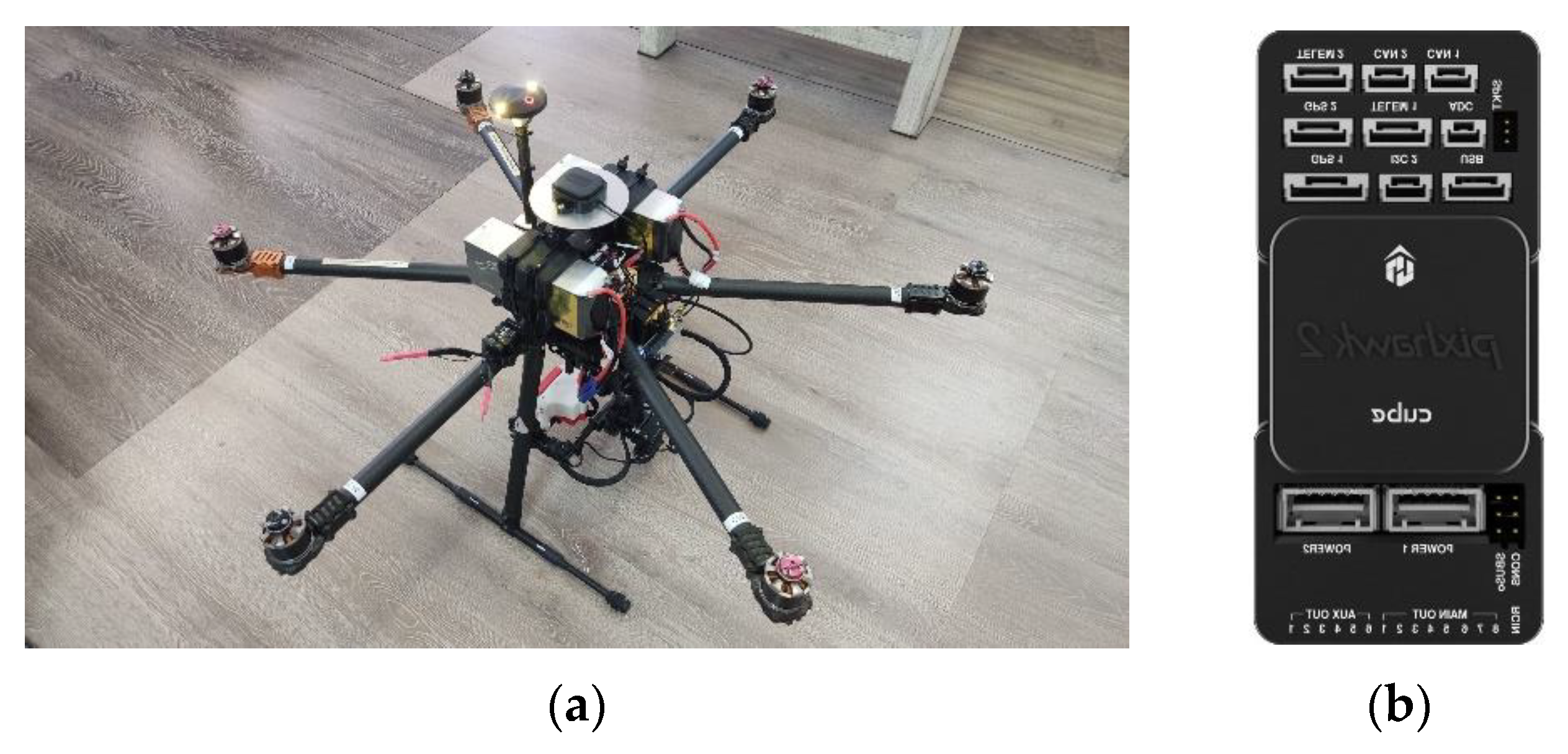
The target deployment platform selected for this study is a custom-made hexacopter UAV (Figure 1). The aircraft body is primarily made out of carbon-fiber composite components to provide structural strength, while maintaining low weight.
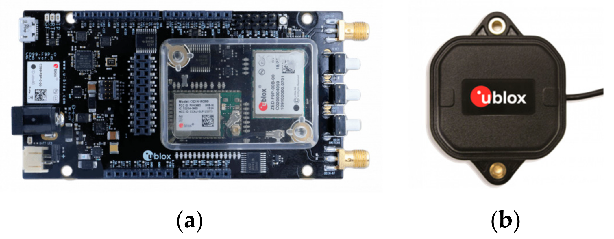
This aerial platform is capable of carrying payloads up to 4 Kg, while enabling complete customization regarding the on-board equipment arrangement. This aircraft features a Pixhawk 2 Cube flight control unit (FCU) [30] to control the aircraft, along with a dual band Ublox F9P [31] GNSS receiver, which provides the system with global positioning data (Figure 2). This RTK enabled GNSS solution is able to provide centimeter level accuracy when corrections are available.
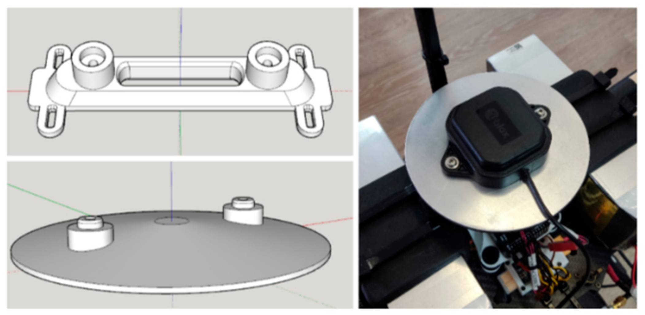
To aid the GNSS signal reception, the dual band antenna is mounted on a 0.5 mm thickness by 120 mm diameter aluminum disk, on top of the aircraft. The disk acts as a ground plane and mitigates unwanted multipath effects [32]. As the disk is made from a non-ferromagnetic material (aluminum), it does not interfere with the magnetic compass of the aircraft. The mount was custom designed and 3D printed (Figure 3).
The selected processing block for the system is a Raspberry Pi 4 (RPi4) [33] embedded computer. This single board computer was selected as it features a relatively “low-power”, “low-weight” design with many available interfacing options. This module is the core of the system as it is responsible of continuously executing the localization task and updating the flight controller in real-time with the calculated data. The computer also interfaces both the GNSS unit and visual-depth camera, which feed the localization algorithm with vital data.
The selected visual-depth sensor is an Intel RealSense D435 camera sensor [34], which has built-in depth estimation functionality (Figure 4). Moreover, the sensor also features an active IR projector to further aid in the depth estimation process [35]. The module interfaces with the RPi4 via USB 3. To install the sensor onto the aircraft, a custom mount was designed and 3D printed (Figure 4).
2.1.2. Robotic Operating System (ROS)
The operation of the localization module is based on processing of many distinct data streams conveying global positioning, visual-depth and inertial data. In order to build the system as a module which can be integrated in modern UAVs and communicate at protocol level with a vast variety of commercial and even industrial sensors, the software is built on top of the Robotic Operating System framework [36,37].
ROS is built to provide a modular approach for robotic applications. Developing individual functional blocks can be very helpful, especially when designing high complexity applications. This approach allows for straightforward development, as each block has a very specific task. An application is constructed after combining the developed blocks in a top-level design. Being able to compose applications through the use of modular design can further aid future expansion of the application under the integration of new functionalities.
2.1.3. ORB-SLAM2
The developed SLAM-based localization processing block is structured as a ROS node in the system environment. It utilizes the ORB-SLAM2 algorithm [24] as it allows the execution of SLAM tasks on monocular, stereo and RGB-D data. The developed localization module expands the initial functionality of the ORB-SLAM2, as it allows further integration of inertial data. In this system, the algorithm receives as input visual-depth data provided by the D435 sensor along with inertial data provided by IMUs of the aircraft.
2.2. Architecture
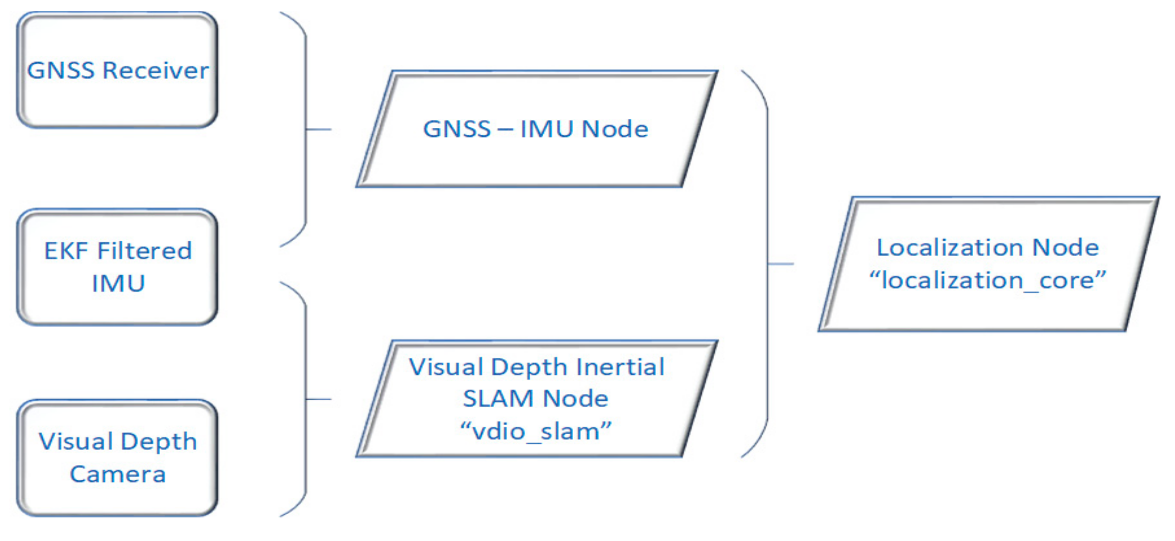
The developed system is built as an ROS package named “sense_nav”, in order to allow integration in modern UAVs. The operation of the system is distributed into two ROS nodes. The first one is called “localization_core” and the second one is called “vdio_slam”. Inside the ROS environment, available data streams convey vital information regarding position and orientation estimations of the UAV. The role of the localization_core node is to monitor the quality of these estimations for each available system and decide which one will be used for localization. The system must support estimations provided primarily by GNSS, while allowing other nodes to provide localization estimations as secondary sources. Such a node is the vdio_slam, which provides localization based on visual, depth and inertial SLAM (Figure 5).
2.2.1. Architecture—The Localization_Core ROS Node
The operation of this node is highly important as it needs to continuously monitor the available streams in order to be always up-to-date, regarding both the localization availability and quality. Moreover, it is the responsibility of this node to feed the flight control unit with localization data.
As the node initializes, the origin (0, 0, 0) (X, Y, Z) of the local three-dimensional space is referenced with global coordinates of a fixed point described in the form of WGS84 (latitude, longitude, altitude). This process can be done either automatically or manually. The system is able to accept as origin the first valid GNSS fix, which also satisfies the quality parameters set by the user. In addition, the origin point can be supplied to the system as a user-specified parameter.
The navigation system of this study complies with the rules of REP 103 [38] and REP 105 [39], hence the East North Up (ENU) convention is used for referencing the local three-dimensional space. As many geometric calculations need to be conducted between many reference frames, the TF [40] transform library is utilized.
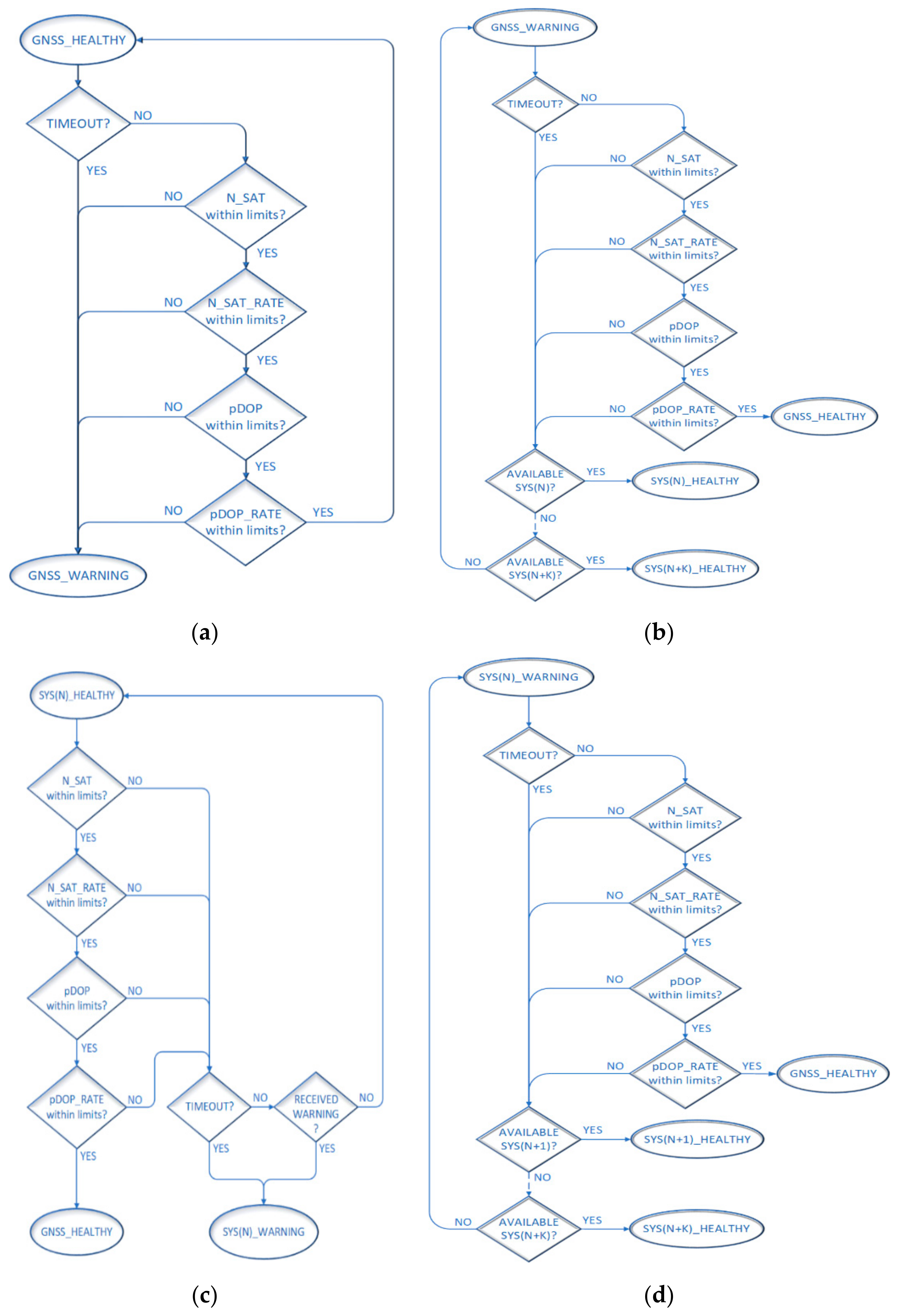
The localization_core operates as a multiplexer controlled by a state machine. By monitoring the available localization streams, it selects as the systemwide localization source the system with the highest priority which also reports healthy status. The system with the highest priority is the GNSS. Next, the SYS_0 input source follows, leaving SYS_N as the input source with the lowest priority. SYS_0 and SYS_N are sources that can be supplied by other nodes such as the vdio_slam, which was designed and implemented for the purposes of this study. SYS_N is an input source for further interfacing with other localization nodes. The proposed architecture allows for ease of scaling as many localization subsystems can by attached. The selection of the source is made based on the availability and the priority selected by the user. The architecture follows the convention that a higher N number implies lower priority. As the node monitors the available streams, it can be in one of the following states (Figure 6):
- GNSS HEALTHY: GNSS provides reliable data
- GNSS WARNING: GNSS provides unreliable data
- SYS_0 HEALTHY: SYS_0 provides reliable data
- SYS_0 WARNING: SYS_0 provides unreliable data
- SYS_N HEALTHY: SYS_N provides reliable data
- SYS_N WARNING: SYS_N provides unreliable data
Figure 6.
The states of the localization_core node, along with their possible transitions. A detailed explanation of the transition logic can be found in Figure 7.
Figure 6.
The states of the localization_core node, along with their possible transitions. A detailed explanation of the transition logic can be found in Figure 7.

The localization_core broadcasts, continuously and in a systemwide fashion, its status containing the latest valid localization data. The idea is that other nodes will be able to receive such data and update their internal knowledge regarding the localization state. Those nodes will continuously report their latest positioning estimations and status to the localization core, and in the case a warning arises on one subsystem, another one can take over.
The system can be configured to operate based on GNSS measurements when certain criteria are satisfied. As other studies suggest [41,42], the position dilution of precision (pDOP) value can be a considerable metric when evaluating GNSS positioning data. The criteria selected for this study are the utilized satellite count and the pDOP value, supplied by the GNSS receiver. The configurable parameters are:
- Minimum satellites count: The minimum number of satellites which are considered acceptable for positioning regarding a specific flight.
- Minimum satellite count drop rate: This value indicates the satellite count drop rate, which triggers the GNSS_WARNING state.
- Maximum pDOP: The maximum pDOP value which is considered tolerable regarding a specific flight.
- Minimum pDOP increase rate: This value indicates the pDOP increase rate, which triggers the GNSS_WARNING state.
- IMU/GNSS/(other localization source, e.g., vdio_slam) timeout: The amount of time in milliseconds which triggers a timeout event, indicating that a module has become unresponsive. Each module can be configured individually.
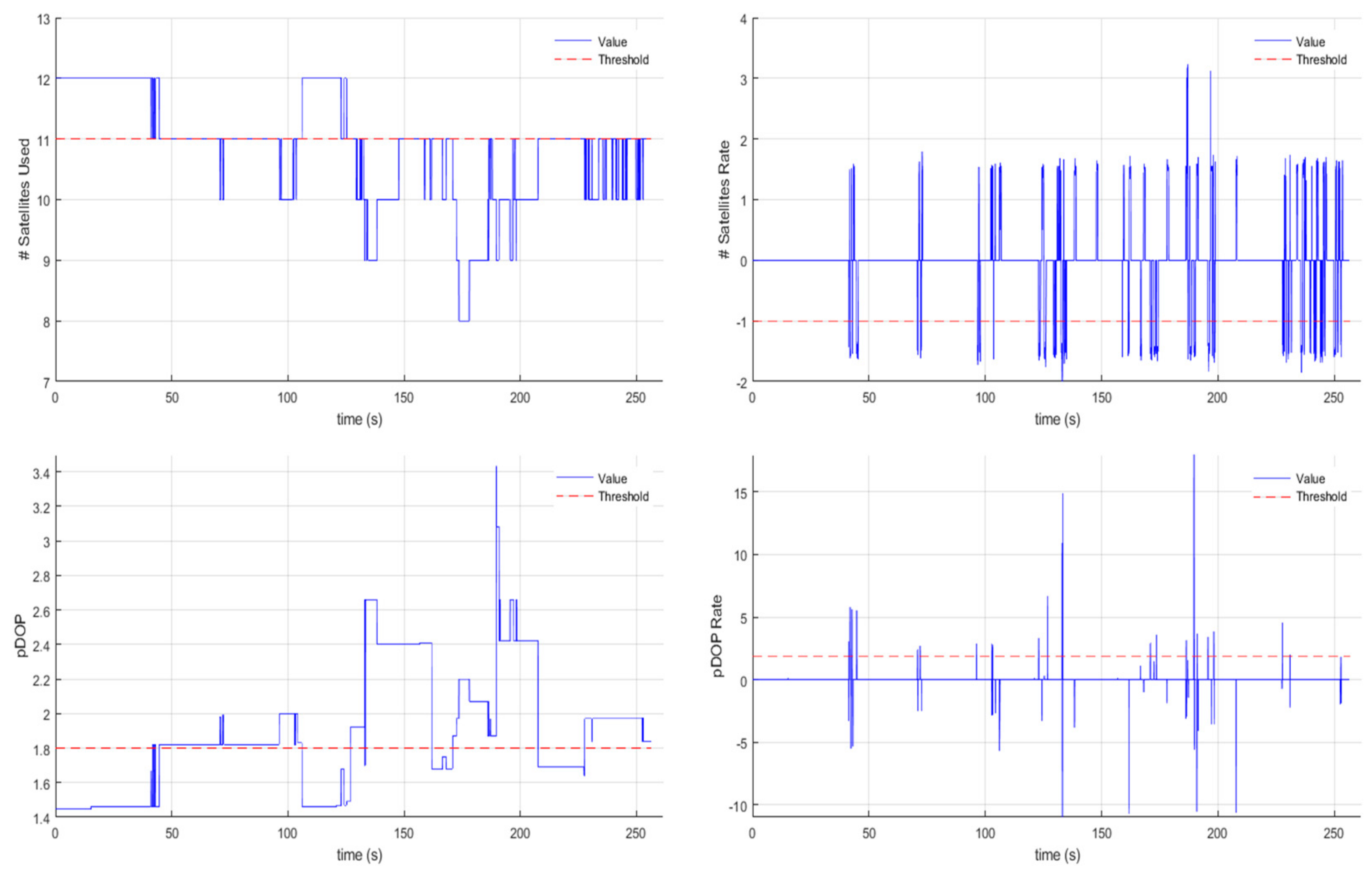
Selecting the thresholds is a vital task, as they determine the stability of the system. The thresholds regarding the number of satellites used, as well as the pDOP, depend on the selected constellations. In this study, the GNSS receiver utilizes GPS and Galileo satellites. The lowest satellite count reported by the receiver during a time window of about 2 h was never bellow 12 satellites, while the pDOP was constantly lower than 2. As the UAV was maneuvered closer to buildings, some satellite signals were obstructed which resulted in an instant decrease in the number of satellites used followed by an increase of the pDOP value. Hence, an appropriate threshold value for the minimum satellite count should be the lowest observation—1. The maximum pDOP for a similar setup should be set as close to 2, as such a value was found to provide a great confidence level. Selecting the thresholds regarding the rates is an optional step, which requires further testing as those rates are not only affected by the surrounding area, but also from the velocity of the aircraft and the output rate of the GNSS receiver.
Figure 7.
State transition logic of the localization_core. Diagrams (a,b) indicate the state transition logic when the system is in GNSS_HEALTHY or GNSS_WARNING state, whereas diagrams (c,d) describe the transition logic when other localization systems are either in SYS_N_HEALTHY or SYS_N_WARNING. N_SAT is the current value of number of satellites used, and N_SAT_RATE is the current value of the overtime change of N_SAT. In a similar fashion, pDOP_RATE is the current value of the overtime change of Position Dilution of Precision (pDOP).

This node houses two callback queues, handled by two individual threads. In the primary queue, the callbacks that are related to the selected localization source are assigned, while the rest are allocated to a secondary queue for monitoring purposes. After each time the localization system changes, the assigned callbacks on those two threads are also adjusted. This design results in the minimum amount of dropped messages.
2.2.2. Architecture—The Vdio_Slam ROS Node
Operating a UAV in GNSS-denied environments can be challenging. In order to tackle such scenarios, a SLAM ROS node was created. This node is named vdio_slam as it uses visual, depth and inertial data to provide odometry readings. Vdio_slam is primarily based on the ORB_SLAM2 algorithm.
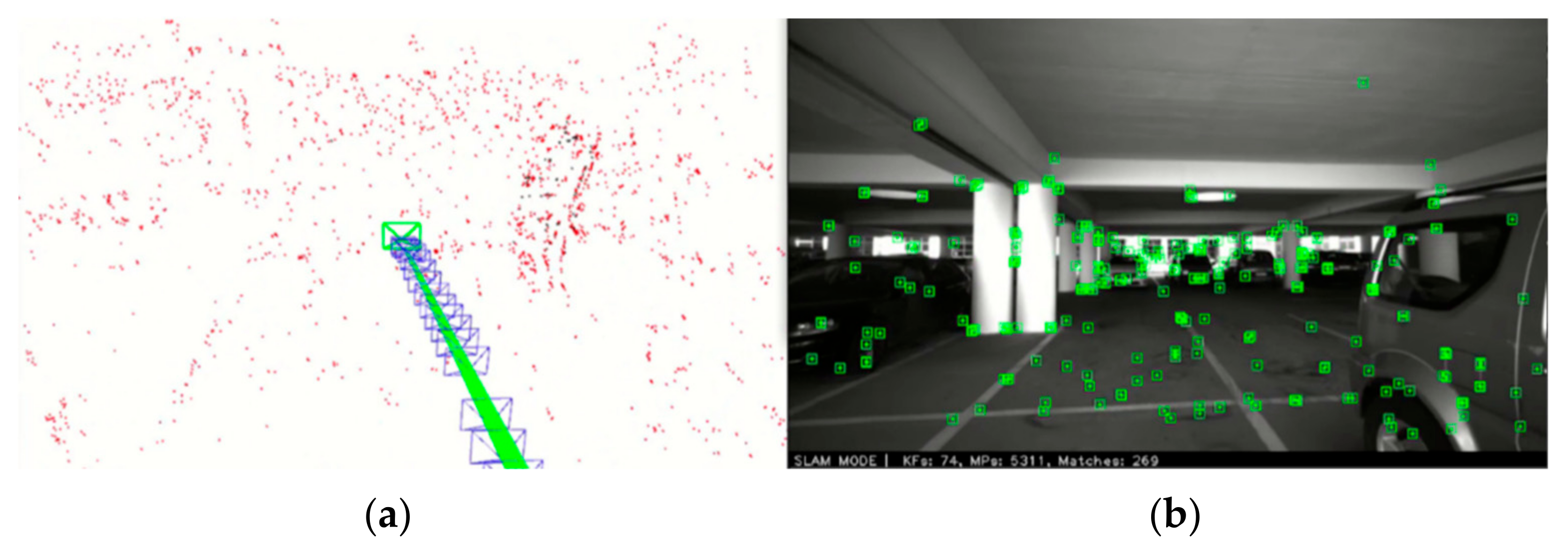
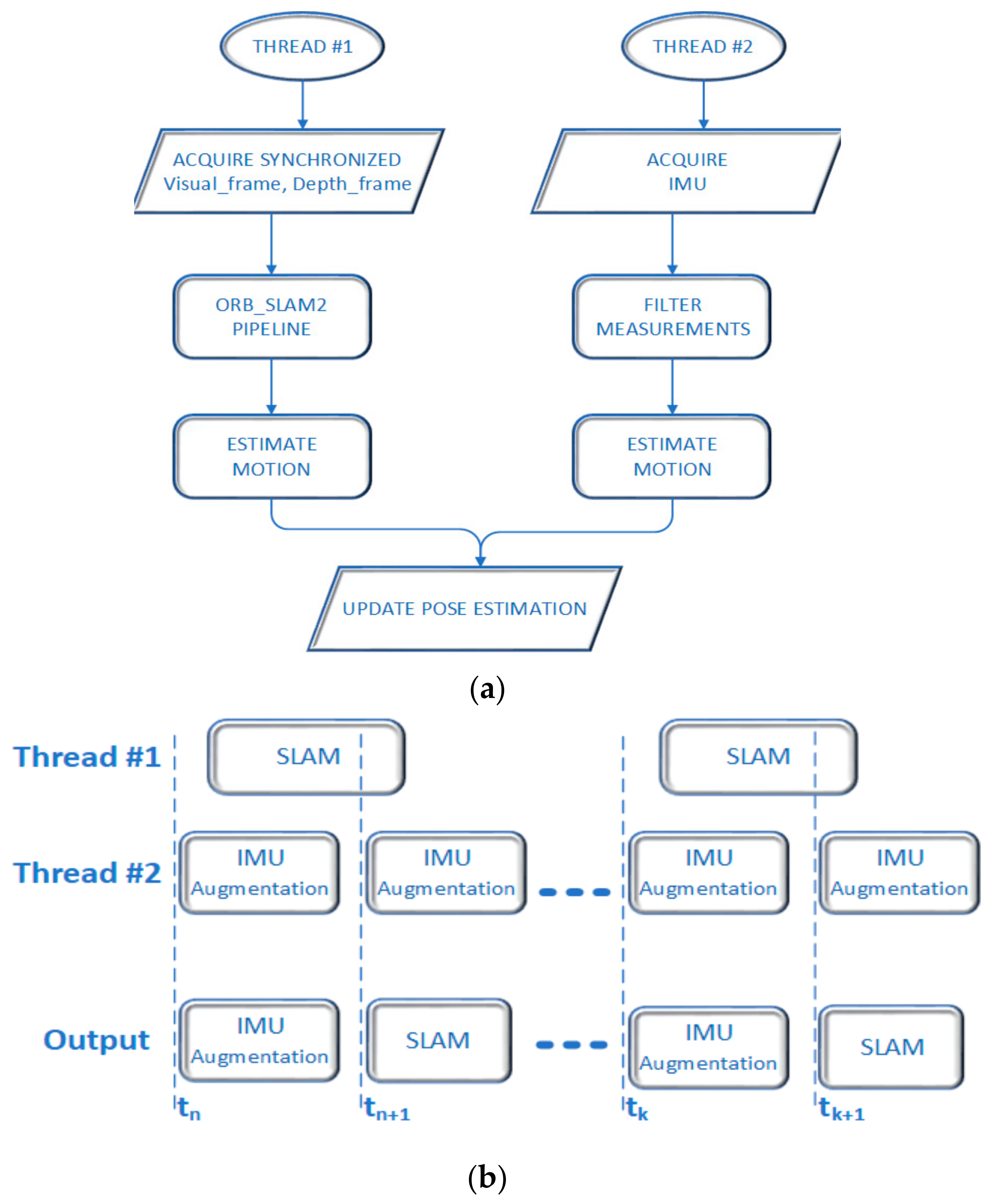
By utilizing this node, the UAV is able to gain spatial awareness by moving through space and acquiring visual features as spatial points of reference (Figure 8). The input streams of this node are the visual and depth frames of the RGB-D sensor, as well as the IMU data stream of the UAV.
The visual and the depth streams are fed directly to the ORB_SLAM2 pipeline. The execution of the algorithm is expensive in terms of performance. After performing tests with the highest resolution settings, the on-board processing unit was able to perform pose estimation on the surrounding area at a rate of 11 Hz. Such performance can be sufficient for positioning use cases. However, many applications require higher rates. Increasing the localization rate can result in higher overall stability of the system.
In order to increase the pose estimation rate, the idea was to take advantage of the IMU data. The flight controller can provide IMU readings at a rate of 30 Hz. Hence, another thread was created to handle the IMU data.
Integrating the readings of acceleration in time, results in velocity. Integrating velocity results in translation. The angular velocity supplied by the IMU was also taken into account. As the ORB_SLAM2 runs on the first thread, the other provides estimations based on the IMU. Each time an ORB_SLAM estimation is calculated, the pose estimation is re-initialized. Between any two ORB_SLAM poses, IMU-based pose estimations are integrated. By taking advantage of the IMU, the output rate of the node reached a stable 30 Hz pose estimation output on the on-board processing unit (Figure 9).
The vdio_slam node interfaces with the localization_core to exchange vital data throughout the flight. As the localization_core reports a GNSS_HEALTHY or SYS_N_HEALTHY state, the vdio_slam resets the pose estimation and sets the origin of the tracking, on the latest reported pose provided by the localization_core. In the case that the localization_core reports a WARNING state and the vdio_slam is able to perform the pose estimation, a HEALTHY output will be forwarded.
3. Testing and Results
3.1. Evaluating the Localization Performance
To evaluate the overall performance of the localization system, actual field tests were conducted. Among the various tests, herein we present various representative experimental results, in GNSS-enabled areas as well as GNSS-denied ones.
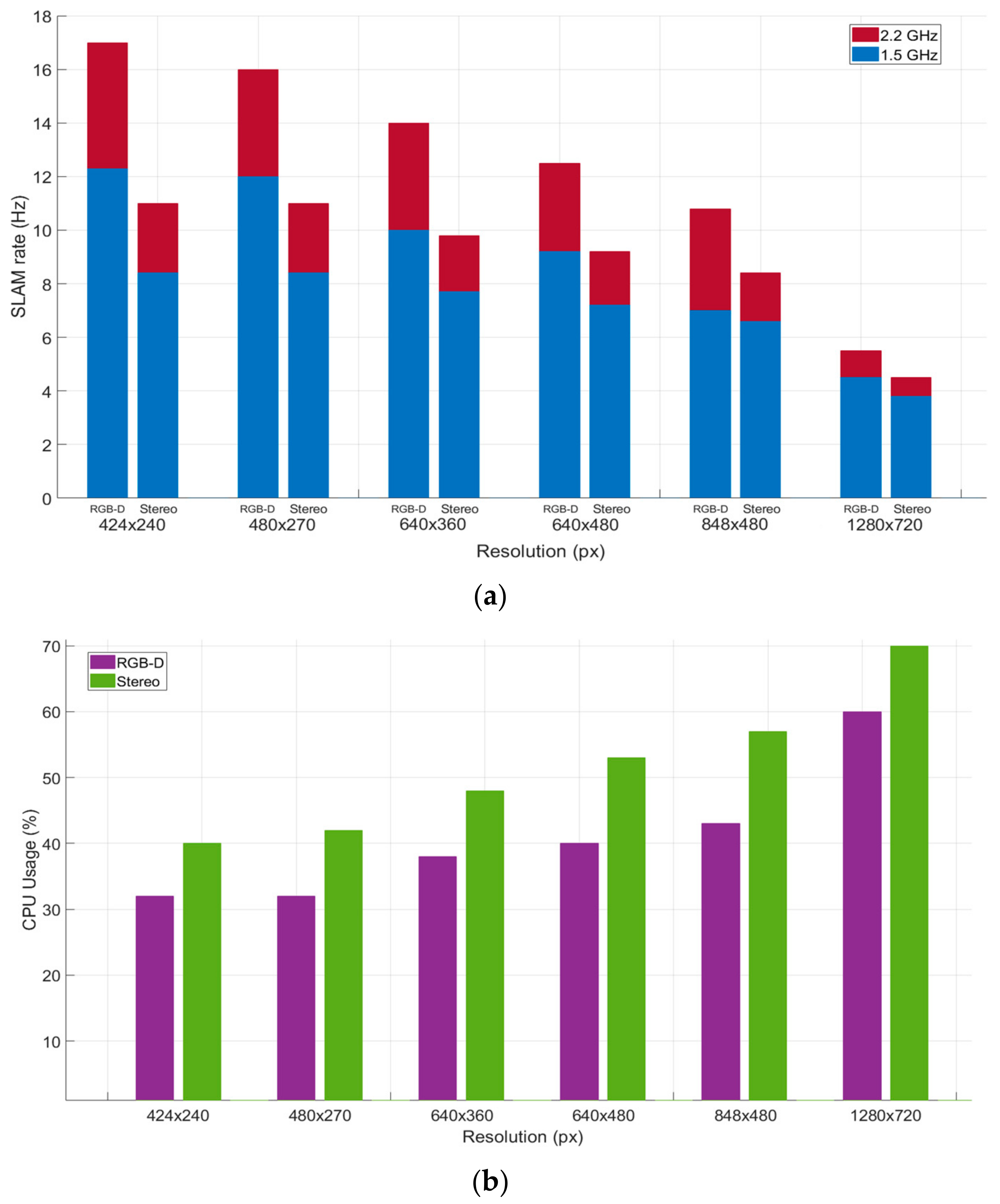
As the proposed localization system runs on a limited performance embedded computer, the Stereo, as well as the RGB-D ORB-SLAM 2 pipelines, were tested in various resolutions and CPU profiles to detect which combination is more viable. The monocular pipeline was not tested as it is a scale-depended solution, whereas both the Stereo and the RGB-D are not, given the camera calibration profiles are known to the system.
By comparing the acquired data (Figure 10), the most appropriate combination for the purposes of this study appears to be the RGB-D pipeline at 848 × 480 resolution when the CPU (ARM Cortex-A72) is clocked at 2.2 GHz, considering that the output rate drops dramatically in a non-linear fashion after this point. Moreover, such combination allows even more than 50% of the CPU to be used for further on-board processing. After selecting such settings, the system was prepared for field testing to evaluate the localization accuracy for different methods.
For the first stage of field testing, a space was selected to conduct some initial tests to evaluate various localization subsystems and techniques. Ground truth points were spread across the selected area and were calculated in a local coordinate system with the utilization of a topographic 3D laser scanner (Leica BLK 360). After re-estimating the coordinates of these points via an RTK-Aided GNSS, the local coordinate frame was converted to ENU. For the purposes of performing an initial evaluation of possible localization methods, the UAV did not perform an actual flight and was rather maneuvered around by hand.
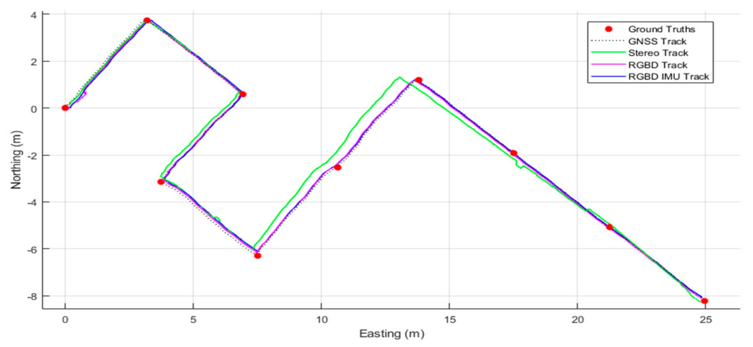
The selected localization methods were an extended Kalman filter (EKF) fused output of GNSS and IMU, an ORB-SLAM2 pipeline operating on Stereo camera streams, an ORB-SLAM2 pipeline operating on RGB-D streams, and the vdio_node which augments the ORB-SLAM2 RGB-D pipeline with the integration of EKF-IMU data.
After initializing the UAV as close as possible to the first ground truth point, the UAV was maneuvered along the evaluation track, over the established ground truth points. During those tests, no algorithms were reset or re-initialized. Throughout the test, the UAV was at a constant height of about 2 m above ground, while maintaining its initial orientation at a low speed of around 3 m/s. In Figure 11 and Table 1, some essential data regarding tested localization methods are provided.
Such initial data suggest that in terms of accuracy regarding the SLAM pipelines operation on the D435 streams, the RGBD appears to obtain the highest accuracy and lowest angular drift; hence, the vdio_node was developed, which appears to provide even higher accuracy by integrating EKF filtered inertial data. In the next stage of field testing, the vdio_node was put to further testing by performing an actual flight in a GNSS-enabled area.
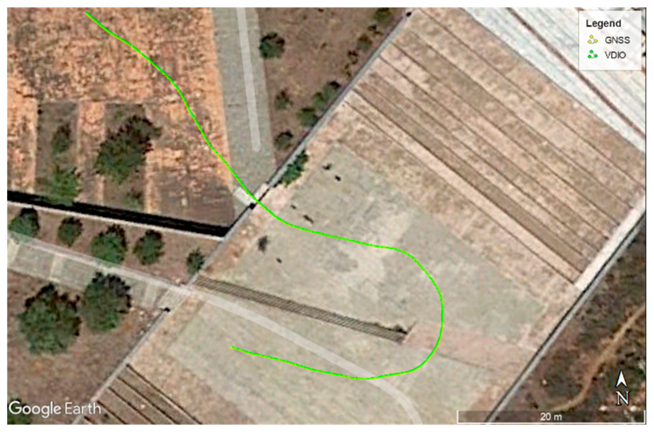
After taking off, the UAV followed a curved path in a GNSS-enabled area in which RTK corrections were also available by a nearby base-station. The calculated positioning data provided by the RTK-GNSS were used as ground truth points. The vdio_slam was initialized right after the first successful RTK augmented fix. For testing purposes, the algorithm was forced to deny re-initialization. This test took place in daylight under moderate sunlight exposure.
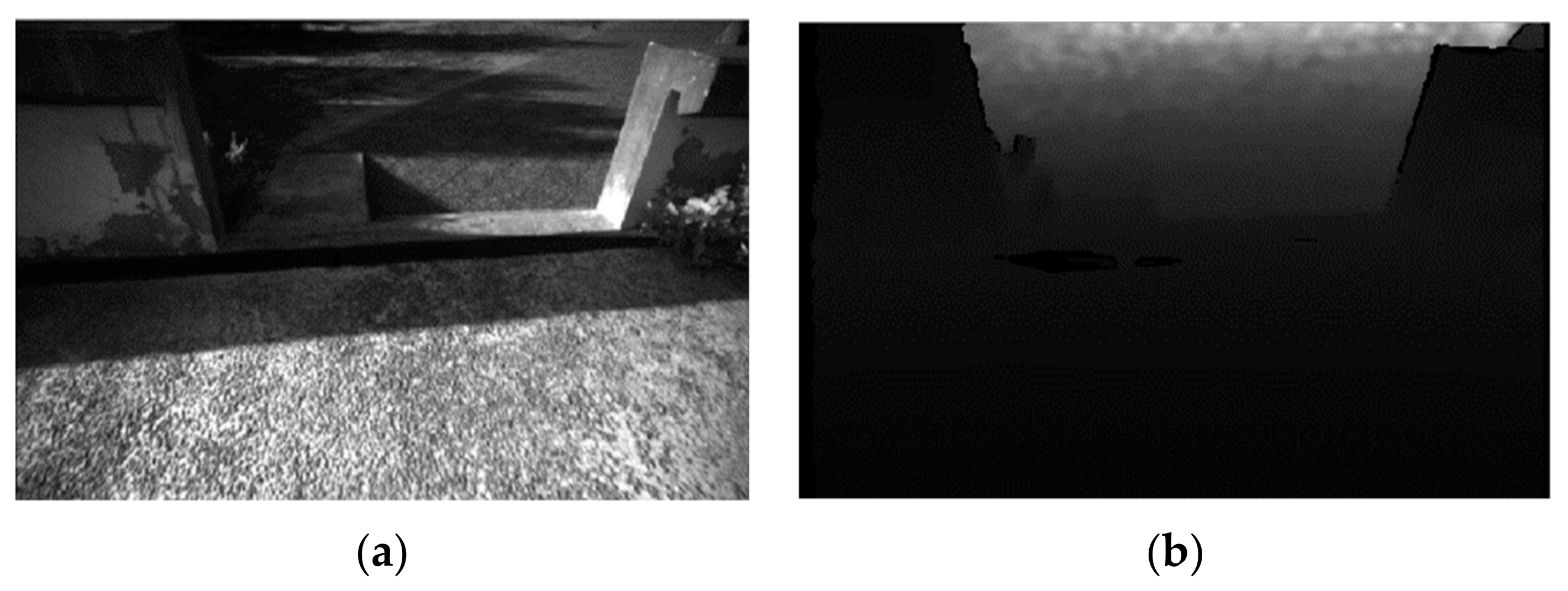
Throughout the flight, the RGB-D sensor was able to provide both visual and depth data (Figure 12) at a stable rate of 12 Hz, while the IMU was feeding the algorithm in a constant rate of 30 Hz.
As indicated in the recorded GNSS data (Figure 13), the system was operating in a GNSS-enabled environment and RTK corrections were utilized throughout the flight. The number of satellites used never dropped below 12 and the pDOP did not report values above 1.5. GNSS status was constantly reported as “2”, indicating the continuous usage of RTK corrections via the ground-based augmentation system. The values of GNSS status, the number of satellites used and pDOP are directly reported via the GNSS module (Ublox F9P). Possible GNSS status values are:
- −1: Unable to fix position
- 0: Unaugment fix
- 1: Satellite-based augmentation
- 2: Ground-based augmentation
3.2. Flying in GNSS Challenging Areas
After the initial tests of the system in GNSS-enabled environments, the UAV was put to the test in more challenging flight scenarios. Tests were conducted in order to evaluate the performance of the localization module in GNSS challenging environments.
To provide referenceable testing data, ground truth points were spread across the testing areas and were registered with the utilization of a 3D laser scanner (Figure 17), as healthy GNSS signals could not be obtained. The reported 3D accuracy of the ground truths is 0.004 m.
For the purposes of multi-environment testing (Figure 18) evaluation, two flights are presented. The flights were initialized in the same area where the localization accuracy was evaluated. Both flights presented were commenced in a location where a stable GNSS-RTK fix could be established.
In the first flight, right after the takeoff, the UAV entered a GNSS-challenging environment. The flight area was abundant with GNSS “blind spots” (Figure 19), making it impossible for satellite signals to be received sustainably.
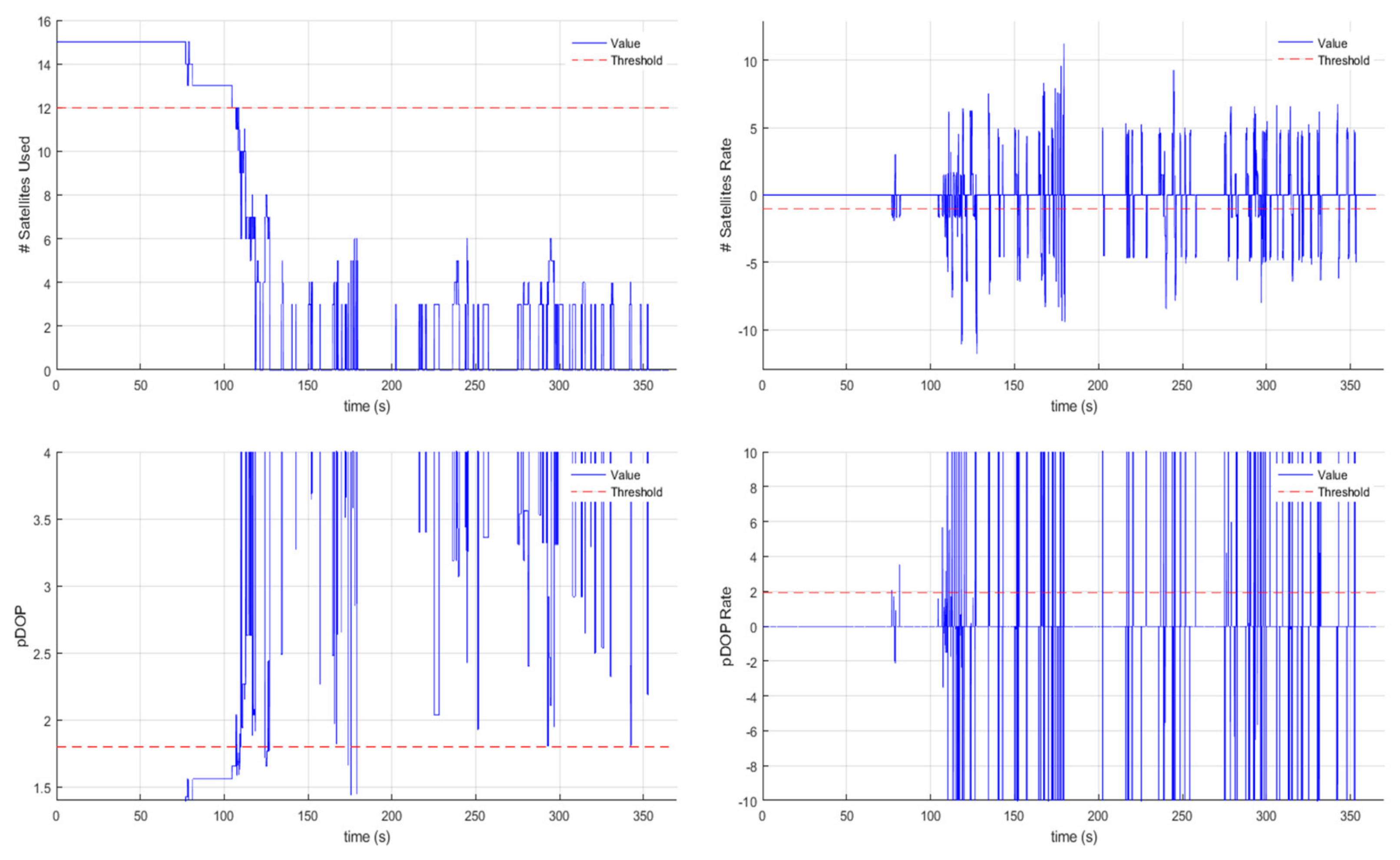
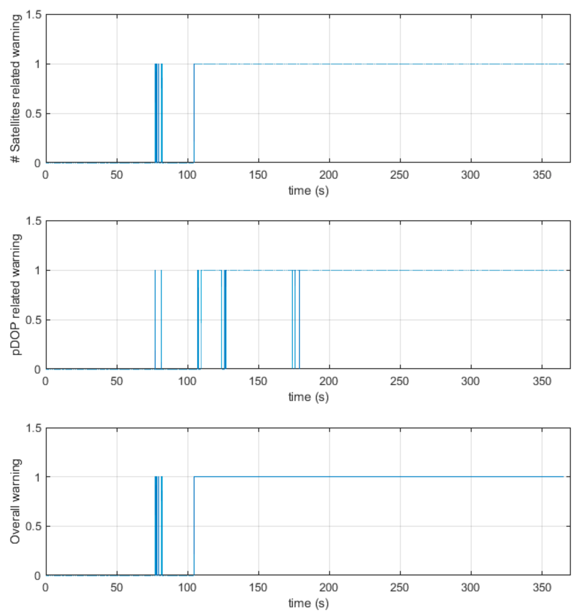
As indicated in the recorded GNSS data (Figure 20 and Figure 21), the system was able to initially utilize the GNSS as the localization source; however, the GNSS reported many instabilities during the flight in the selected area. The number of satellites used was continuously changing, as did the reported pDOP. During this test at around t = 150 s, the UAV entered a concrete ceiling corridor (Figure 19). Inside the corridor, the pDOP reached a peak value of 3.4, and the available satellite count dropped to 8. The recorded satellite count and pDOP rates can be found in Figure 20 with their selected operating thresholds.
In this flight, the UAV was maneuvered over the ground truth points to allow for accuracy evaluation in actual conditions. The localization system was able to select the GNSS–IMU submodule as the localization source during only the initial and middle stages of the flight. The reception of the GNSS signals was immediately degraded after entering the testing zone. However, the system was able to maintain spatial awareness as the vdio_slam was able to execute uninterruptedly. The acquired trajectory of the UAV can be seen in Figure 22.
A total of 25 ground truth points were utilized to evaluate the accuracy of this experiment. In this experiment, the system was operating on GNSS-IMU data from the initial point (ground truth #1). The vdio_slam was continuously re-initialized to the latest available GNSS fix and was handed over the localization task initially near ground truth point #5, up until around point #12, where a healthy GNSS fix could be obtained. Near ground truth point #14, the localization task was once again handed over to the vdio_slam, which was re-initialized to the latest GNSS fix. This test was concluded shortly after passing over the ground truth point #25. The accuracies acquired regarding this experiment can be found below (Table 2).
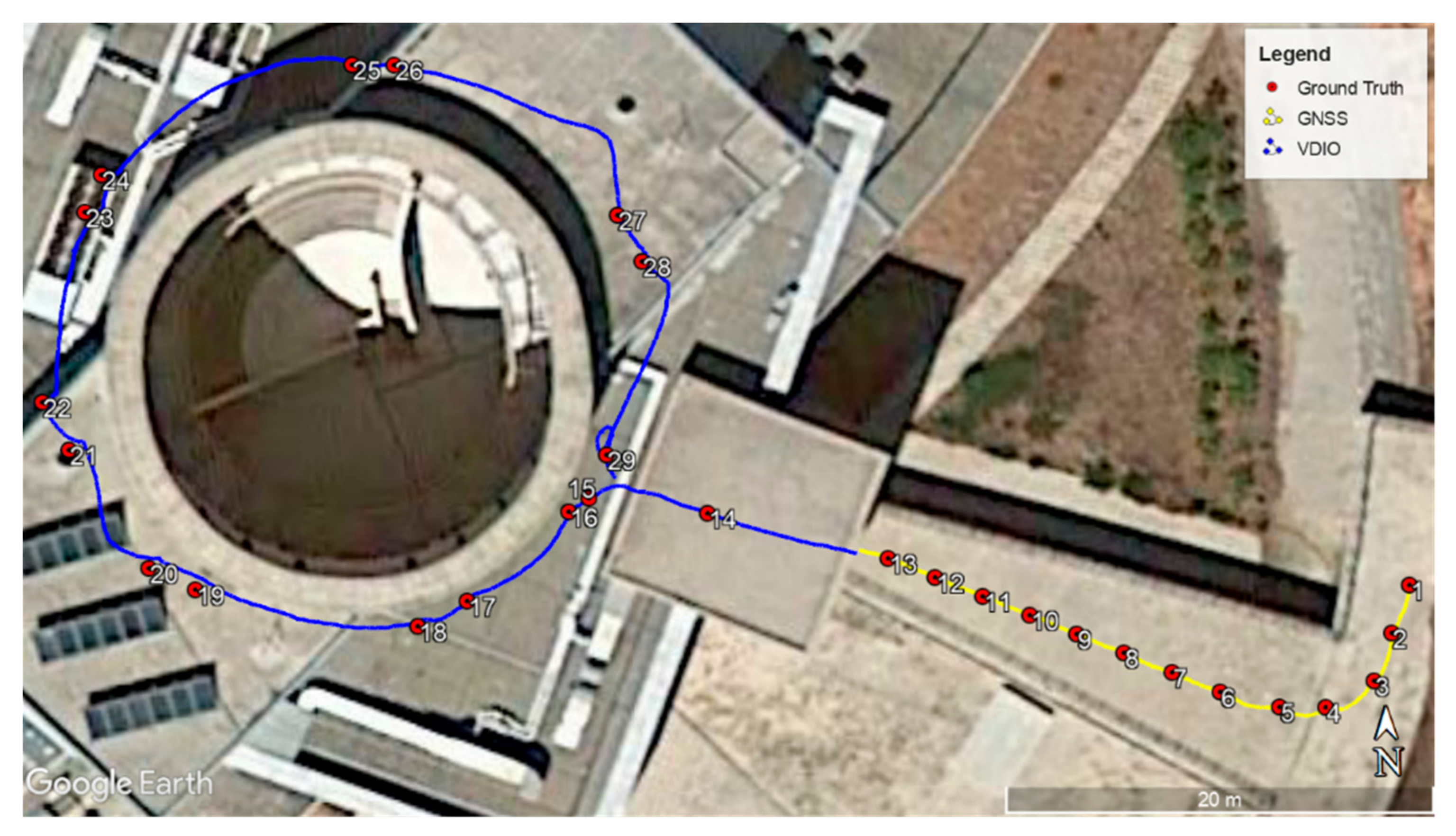
Another experiment was conducted in a nearby area to further investigate the accuracy of the system inside a GNSS-denied area, which is the inside of a building. In that scenario, the UAV was once again initialized in a GNSS-RTK enabled area. A total of 29 ground control points were spread in the area of interest, both inside and outside of the building.
In the initial stage of the predetermined trajectory, the UAV was maneuvered over an unclouded open space before entering the building. As indicated by the recorded GNSS data (Figure 23 and Figure 24), the system was operating initially inside an area of adequate GNSS-RTK coverage up until the ground truth point #13 (Figure 25), near t = 105 s. At that point, the UAV entered the building and the GNSS vitals were quickly degraded (Figure 23).
While entering the building, the thresholds were surpassed (Figure 23 and Figure 24), and the vdio_slam was handed over the localization task. The vdio_slam was continuously re-initializing at each healthy GNSS fix before this point. After entering the building, the vdio_slam did not re-initialize until the completion of the experiment.
This experiment was concluded right after the UAV passed over the ground truth point #29. As suggested by the acquired trajectory (Figure 25), the UAV was able to provide sufficient localization inside the building. The calculated accuracies of this experiment can be found in the table below (Table 3).
4. Discussion and Conclusions
4.1. Discusion on the Main Findings
The developed system is able to provide sufficient localization data even in GNSS-challenging environments. In order to supply the UAV with appropriate localization estimations, the system initially evaluates the quality of the data acquired via GNSS, as they are the primary source of positioning estimations. In case the GNSS data are determined as “low” in quality, a SLAM algorithm is initialized at the latest known high quality position fix. The SLAM algorithm takes visual, depth and inertial data, and provides a globally referenced localization output.
As mentioned in Section 2, the system needs to continuously monitor the quality of the GNSS data and select the localization source accordingly. In order to evaluate the quality of the GNSS data, the algorithm takes into account the pDOP value and the number of utilized satellites. Moreover, in order to determine possible GNSS signal degradation in a timely manner, thresholds are applied even in the rate of change of both the satellite count and the pDOP value.
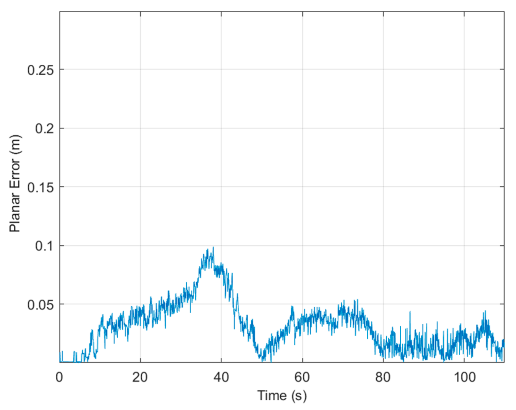
Regarding the experiments mentioned in Section 3, the system was initially able to output sufficient localization data, as it was operating in a GNSS-enabled area and RTK corrections were also available. The SLAM-estimated UAV trajectory was able to follow the RTK-GNSS track with a very low planar error of less than 0.1 m for the whole duration of the evaluation flight. The SLAM was able to provide pose estimation based on the visual-depth streams at a rate of 12 Hz, which is about the same rate reported by the F9P GNSS receiver. The IMU of the aircraft was able to supply the algorithm with 30 Hz inertial measurements. By integrating the inertial measurements between the visual-depth SLAM estimations, the system was able to perform stably at 30 Hz, doubling the initial rate. It is worth mentioning that the whole system was executing on a low power ARM-based single board computer (RPi4). The selected visual-depth resolution on which the SLAM was successfully conducted was 848 × 480 p.
In order to save processing power and memory without sacrificing positioning accuracy, the SLAM was continuously reinitialized to the latest known high quality position fix. In the case that the system entered the GNSS-WARNING state, the SLAM would immediately stop the reinitializing process and execute uninterruptedly until the system reported the GNSS-HEALTHY state, which would trigger once again the reinitialization of the SLAM.
During the initial test, the thresholds which assess the GNSS quality were selected and evaluated in later flights inside GNSS-challenging areas. The minimum tolerable satellite count was set to 12 and the minimum satellite count drop rate to 1.0. The maximum pDOP was set at 1.8, while the selected minimum pDOP increase rate was 2.0.
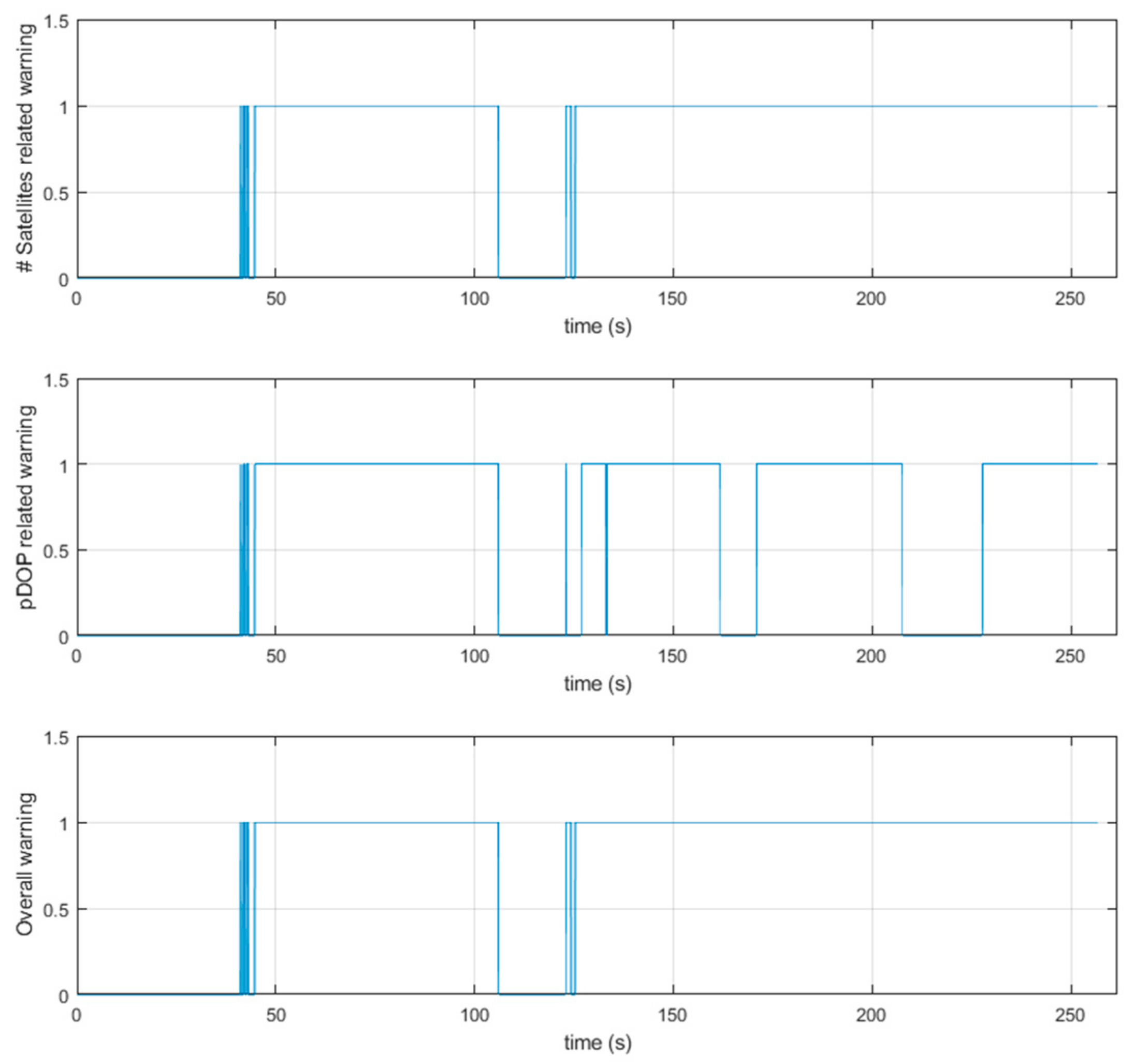
Regarding the first test inside a GNSS-challenging zone (t = 40 s), the system immediately reported the GNSS-WARNING state and the SLAM became operational in less than 50 ms. While the UAV was inside the GNSS-challenging area, it was unable to switch back to the GNSS-HEALTHY state as at least one threshold was surpassed or the GNSS reported 0 status. As suggested by the recorded data (see Figure 20, Figure 21 and Figure 22), the GNSS track indicates that the receiver was not able to provide a reliable fix continuously inside the GNSS-challenging environment. It reported many instabilities as abrupt satellite count drops followed by instantaneous pDOP increases. It is worth noting that around time t = 150 s, as the UAV entered the concrete ceiling corridor, the GNSS readings were highly degraded, and even reported a false right-hand turn after the UAV exited the corridor. On the contrary, the vdio_slam was able to perform adequately as the track acquired had no indications of instabilities or discrete “jumps”, but rather a smooth continuous path.
Similar performance was observed also on the second test in GNSS-challenging areas. The system immediately sensed the drop in satellite count, and did not re-initialize the vdio_slam from that point on, until the end of the experiment.
For both experiments, we can conclude that the most important threshold was the available satellites number, as it was found to be the decisive factor. The thresholds regarding the rates were found to function properly as early warnings of a possible future decrease of GNSS integrity.
4.2. Future Work
Despite the proven abilities of this system, there is always room for improvements, as well as added functionality. The system was designed in this configuration in order to allow expandability as further functionality can be integrated in the form of ROS nodes. The localization_core node has been already implemented with an unconnected port for another localization submodule. Such a module can be an extended Kalman filter (EKF) core, which may take as input different combinations of the available localization data. Despite the expected increase in position estimation accuracy, the whole system will be capable of calculating even more flight parameters, such as linear and angular velocities.
Currently, the mechanism which determines the quality of the selected attributes is a set of thresholds. Despite being effective, it requires tuning. This aspect could be improved if deep learning methods were introduced. Recurrent neural networks (RNNs) appear as exceptional candidates for this operation as they can operate on timeseries. In such architecture, an RNN may take as input the timestamped sequence of both utilized satellite number, as well as the pDOP value, and provide a single output which will be used to control the switching operation between GNSS_HEALTHY and GNSS_WARNING.
Finally, from an embedded software architecture design perspective, the system should be ported in ROS_2. By migrating to ROS_2, the system can benefit in terms of higher performance data processing for every designed node [43,44]. Given that the system is designed as core component for modern UAVs, accurate synchronization is also required. In such a scenario, ROS_2 can satisfy the synchronization needs [45].
Author Contributions
Conceptualization, A.A. and P.P.; methodology, A.A., M.G.L. and P.P.; software, A.A.; validation, A.A. and P.P.; formal analysis, A.A.; writing—original draft preparation, A.A. and P.P.; writing—review and editing, A.A., M.G.L. and P.P.; visualization, A.A.; funding acquisition, P.P. All authors have read and agreed to the published version of the manuscript.
Funding
This research has been co-financed by the European Union and Greek national funds through the Operational Program Competitiveness, Entrepreneurship and Innovation, under the call RESEARCH–CREATE–INNOVATE (project code: T1EDK-03209).
Institutional Review Board Statement
Not applicable.
Informed Consent Statement
Not applicable.
Data Availability Statement
No publicly available data were used or generated.
Conflicts of Interest
The authors declare no conflict of interest.
Abbreviations
| EKF | Extended Kalman Filter |
| ENU | East North Up |
| FCU | Flight Control Unit |
| GNSS | Global Navigation Satellite Systems |
| IMU | Inertial Measuring Unit |
| KF | Kalman Filter |
| pDOP | Position Dilution of Precision |
| RF | Radio Frequency |
| RGB-D | Red Green Blue-Depth |
| ROS | Robotic Operating System |
| RPi | Raspberry Pi |
| RTK | Real-Time Kinematics |
| SLAM | Simultaneous Localization and Mapping |
| UAV | Uncrewed Aerial Vehicle |
References
- Kortunov, V.I.; Mazurenko, O.V.; Gorbenko, A.V.; Mohammed, W.; Hussein, A. Review and comparative analysis of mini- and micro-UAV autopilots. In Proceedings of the 2015 IEEE International Conference Actual Problems of Unmanned Aerial Vehicles Developments (APUAVD), Kyiv, Ukraine, 13–15 October 2015; pp. 284–289. [Google Scholar]
- Hulens, D.; Verbeke, J.; Goedemé, T. Choosing the Best Embedded Processing Platform for On-Board UAV Image Processing. In Computer Vision, Imaging and Computer Graphics Theory and Applications; Communications in Computer and Information Science; Springer: Cham, Switzerland, 2016; p. 598. [Google Scholar]
- Droeschel, D.; Behnke, S. Efficient Continuous-Time SLAM for 3D Lidar-Based Online Mapping. In Proceedings of the IEEE International Conference on Robotics and Automation (ICRA), Brisbane, Australia, 21–25 May 2018; pp. 5000–5007. [Google Scholar]
- Nex, F.; Remondino, F. UAV for 3D mapping applications: A review. Appl. Geomat. 2014, 6, 1–15. [Google Scholar] [CrossRef]
- Doherty, P.; Rudol, P. A UAV Search and Rescue Scenario with Human Body Detection and Geolocalization. In Proceedings of the AI 2007: Advances in Artificial Intelligence, Gold Coast, Australia, 2–6 December 2007; p. 4830. [Google Scholar]
- Kyristsis, S.; Antonopoulos, A.; Chanialakis, T.; Stefanakis, E.; Linardos, C.; Tripolitsiotis, A.; Partsinevelos, P. Towards Autonomous Modular UAV Missions: The Detection, Geo-Location and Landing Paradigm. Sensors 2016, 16, 1844. [Google Scholar] [CrossRef] [PubMed] [Green Version]
- Gyagenda, N.; Hatilima, J.V.; Roth, H.; Zhmud, V. A review of GNSS-independent UAV navigation techniques, Robot. Auton. Syst. 2022, 152, 104069. [Google Scholar] [CrossRef]
- Petritoli, E.; Leccese, F.; Leccisi, M. Inertial Navigation Systems for UAV: Uncertainty and Error Measurements. In Proceedings of the 2019 IEEE 5th International Workshop on Metrology for AeroSpace (MetroAeroSpace), Torino, Italy, 19–21 June 2019; pp. 1–5. [Google Scholar] [CrossRef]
- Zhou, Q.-L.; Zhang, Y.; Qu, Y.-H.; Rabbath, C.-A. Dead reckoning and Kalman filter design for trajectory tracking of a quadrotor UAV. In Proceedings of the 2010 IEEE/ASME International Conference on Mechatronic and Embedded Systems and Applications, Qingdao, China, 15–17 July 2010; pp. 119–124. [Google Scholar] [CrossRef]
- Tiemann, J.; Wietfeld, C. Scalable and precise multi-UAV indoor navigation using TDOA-based UWB localization. In Proceedings of the International Conference on Indoor Positioning and Indoor Navigation (IPIN), Sapporo, Japan, 18–21 September 2017; pp. 1–7. [Google Scholar]
- Li, X.; Ge, M.; Dai, X. Accuracy and reliability of multi-GNSS real-time precise positioning: GPS, GLONASS, BeiDou, and Galileo. J. Geod. 2015, 89, 607–635. [Google Scholar] [CrossRef]
- Hadas, T.; Kazmierski, K.; Sośnica, K. Performance of Galileo-only dual-frequency absolute positioning using the fully serviceable Galileo constellation. GPS Solut. 2019, 23, 108. [Google Scholar] [CrossRef] [Green Version]
- Fengyu, X.; Shirong, Y.; Pengfei, X.; Lewen, Z.; Nana, J.; Dezhong, C.; Guangbao, H. Assessing the latest performance of Galileo-only PPP and the contribution of Galileo to Multi-GNSS PPP. Adv. Space Res. 2019, 63, 2784–2795. [Google Scholar]
- Zhang, G.; Hsu, L.-T. Intelligent GNSS/INS integrated navigation system for a commercial UAV flight control system. Aerosp. Sci. Technol. 2018, 80, 368–380. [Google Scholar] [CrossRef]
- Krajník, T.; Nitsche, M.; Pedre, S.; Přeučil, L.; Mejail, M.E. A simple visual navigation system for an UAV. In Proceedings of the International Multi-Conference on Systems Signals & Devices, Chemnitz, Germany, 20–23 March 2012; pp. 1–6. [Google Scholar]
- Xu, Y.; Pan, L.; Du, C.; Li, J.; Jing, N.; Wu, J. Vision-based UAVs Aerial Image Localization: A Survey. In Proceedings of the 2nd ACM SIGSPATIAL International Workshop on AI for Geographic Knowledge Discovery (GeoAI’18), Seattle, WA, USA, 6 November 2018; Association for Computing Machinery: New York, NY, USA, 2018; pp. 9–18. [Google Scholar] [CrossRef]
- Rosser, K.; Chahl, J. Reducing the complexity of visual navigation: Optical track controller for long-range unmanned aerial vehicles. J. Field Robot. 2019, 36, 1118–1140. [Google Scholar] [CrossRef]
- Liu, X.; Guo, X.; Zhao, D.; Cao, H.; Tang, J.; Wang, C.; Shen, C.; Liu, J. Integrated Velocity Measurement Algorithm Based on Optical Flow and Scale-Invariant Feature Transform. IEEE Access 2019, 7, 153338–153348. [Google Scholar] [CrossRef]
- Du, H.; Wang, W.; Xu, C.; Xiao, R.; Sun, C. Real-Time Onboard 3D State Estimation of an Unmanned Aerial Vehicle in Multi-Environments Using Multi-Sensor Data Fusion. Sensors 2020, 20, 919. [Google Scholar] [CrossRef] [PubMed] [Green Version]
- Abdi, C.; Samadzadegan, F.; Kurz, F. Pose Estimation of Unmanned Aerial Vehicles Based on a Vision-Aided Multi-Sensor Fusion. XXII ISPRS Congress. Tech. Comm. I 2016, 41, 193–199. [Google Scholar]
- Konovalenko, I.A.; Miller, A.B.; Miller, B.M.; Nikolaev, D.P. UAV Navigation on The Basis Of The Feature Points Detection On Underlying Surface. In European Conference on Modelling and Simulation (ECMS); ECMS: Albena, Bulgaria, 2015. [Google Scholar]
- Avola, D.; Cinque, L.; Fagioli, A.; Foresti, G.L.; Massaroni, C.; Pannone, D. Feature-Based SLAM Algorithm for Small Scale UAV with Nadir View. In Proceedings of the Image Analysis and Processing—ICIAP, Trento, Italy, 9–13 September 2019; Volume 11752. [Google Scholar]
- Santamaria-Navarro, A.; Loianno, G.; Solà, J. Autonomous navigation of micro aerial vehicles using high-rate and low-cost sensors. Auton. Robot. 2018, 42, 1263–1280. [Google Scholar] [CrossRef] [Green Version]
- Mur-Artal, R.; Tardós, J.D. ORB-SLAM2: An Open-Source SLAM System for Monocular, Stereo, and RGB-D Cameras. IEEE Trans. Robot. 2017, 33, 1255–1262. [Google Scholar] [CrossRef] [Green Version]
- Bourque, D. CUDA-Accelerated ORB-SLAM for UAVs. Master’s Thesis, Worcester Polytechnic Institute, Worcester, MA, USA, 2017; p. 882. [Google Scholar]
- Yusefı, A.; Durdu, A.; Sungur, C. ORB-SLAM-based 2D Reconstruction of Environment for Indoor Autonomous Navigation of UAVs. Eur. J. Sci. Technol. 2020, 466–472. [Google Scholar] [CrossRef]
- Haddadi, S.J.; Castelan, E.B. Visual-Inertial Fusion for Indoor Autonomous Navigation of a Quadrotor Using ORB-SLAM. In Proceedings of the 2018 Latin American Robotic Symposium, 2018 Brazilian Symposium on Robotics (SBR) and 2018 Workshop on Robotics in Education (WRE), João Pessoa, Brazil, 6–10 November 2018; pp. 106–111. [Google Scholar] [CrossRef]
- Lekkala, K.K.; Mittal, V.K. Accurate and augmented navigation for quadcopter based on multi-sensor fusion. In Proceedings of the 2016 IEEE Annual India Conference (INDICON), Bangalore, India, 16–18 December 2016; pp. 1–6. [Google Scholar] [CrossRef]
- Skoglund, M.; Petig, T.; Vedder, B.; Eriksson, H.; Schiller, E.M. Static and dynamic performance evaluation of low-cost RTK GPS receivers. In Proceedings of the 2016 IEEE Intelligent Vehicles Symposium (IV), Gothenburg, Sweden, 19–22 June 2016; pp. 16–19. [Google Scholar] [CrossRef]
- Cube Flight Controller. Available online: https://docs.px4.io/v1.9.0/en/flight_controller/pixhawk-2.html (accessed on 1 December 2021).
- ZED-F9P Module. Available online: https://www.u-blox.com/en/product/zed-f9p-module (accessed on 1 December 2021).
- Maqsood, M.; Gao, S.; Brown, T.W.C.; Unwin, M.; de vos Van Steenwijk, R.; Xu, J.D. A Compact Multipath Mitigating Ground Plane for Multiband GNSS Antennas. IEEE Trans. Antennas Propag. 2013, 61, 2775–2782. [Google Scholar] [CrossRef] [Green Version]
- Raspberry Pi 4. Available online: https://www.raspberrypi.com/products/raspberry-pi-4-model-b/ (accessed on 1 December 2021).
- Intel Realsense D435. Available online: https://www.intelrealsense.com/depth-camera-d435/ (accessed on 1 December 2021).
- Intel Realsense Projectors. Available online: https://www.intelrealsense.com/wp-content/uploads/2019/03/WhitePaper_on_Projectors_for_RealSense_D4xx_1.0.pdf (accessed on 1 December 2021).
- Robotic Operating System (ROS). Available online: https://www.ros.org/ (accessed on 1 December 2021).
- Quigley, M.; Conley, K.; Gerkey, B.; Faust, J.; Foote, T.; Leibs, J.; Wheeler, R.; Ng, A. ROS: An open-source Robot Operating System. In Proceedings of the ICRA Workshop on Open Source Software, Kobe, Japan, 12–17 May 2009. [Google Scholar]
- ROS REP 103—Standard Units of Measure and Coordinate Conventions. Available online: https://www.ros.org/reps/rep-0103.html (accessed on 1 December 2021).
- ROS REP 105—Coordinate Frames for Mobile Platforms. Available online: https://www.ros.org/reps/rep-0105.html (accessed on 1 December 2021).
- Foote, T. tf: The transform library. In Proceedings of the 2013 IEEE Conference on Technologies for Practical Robot Applications (TePRA), Woburn, MA, USA, 22–23 April 2013; pp. 1–6. [Google Scholar]
- Nie, Z.; Gao, Y.; Wang, Z.; Ji, S. A new method for satellite selection with controllable weighted PDOP threshold. Surv. Rev. 2017, 49, 285–293. [Google Scholar] [CrossRef]
- Teng, Y.; Wang, J. Some Remarks on PDOP and TDOP for Multi-GNSS Constellations. J. Navig. 2016, 69, 145–155. [Google Scholar] [CrossRef] [Green Version]
- da Silva Medeiros, L.; Julio, R.E.; Almeida, R.M.A.; Bastos, G.S. Enabling Real-Time Processing for ROS2 Embedded Systems. In Robot Operating System (ROS); Koubaa, A., Ed.; Studies in Computational Intelligence; Springer: Cham, Switzerland, 2019; Volume 778. [Google Scholar] [CrossRef]
- Puck, L.; Keller, P.; Schnell, T.; Plasberg, C.; Tanev, A.; Heppner, G.; Roennau, A.; Dillmann, R. Performance Evaluation of Real-Time ROS2 Robotic Control in a Time-Synchronized Distributed Network. In Proceedings of the 2021 IEEE 17th International Conference on Automation Science and Engineering (CASE), Lyon, France, 23–27 August 2021; pp. 1670–1676. [Google Scholar] [CrossRef]
- Puck, L.; Keller, P.; Schnell, T.; Plasberg, C.; Tanev, A.; Heppner, G.; Roennau, A.; Dillmann, R. Distributed and Synchronized Setup towards Real-Time Robotic Control using ROS2 on Linux. In Proceedings of the 2020 IEEE 16th International Conference on Automation Science and Engineering (CASE), Hong Kong, China, 20–21 August 2020; pp. 1287–1293. [Google Scholar] [CrossRef]
Figure 1.
(a) The custom hexacopter uncrewed aerial vehicle (UAV) used in this study. (b) The flight control unit of the aircraft, Pixhawk 2 Cube.
Figure 1.
(a) The custom hexacopter uncrewed aerial vehicle (UAV) used in this study. (b) The flight control unit of the aircraft, Pixhawk 2 Cube.

Figure 2.
(a) Ublox F9P Global Navigation Satellite System (GNSS) solution. (b) L1/L2 Ublox ANN-MB GNSS antenna. Source: Ublox (www.ublox.com, accessed on 1 October 2021).
Figure 2.
(a) Ublox F9P Global Navigation Satellite System (GNSS) solution. (b) L1/L2 Ublox ANN-MB GNSS antenna. Source: Ublox (www.ublox.com, accessed on 1 October 2021).

Figure 3.
Mounting the GNSS antenna.

Figure 4.
(a) The visual-depth camera sensor Intel RealSense D435. (b) Mounting the D435 onto the aircraft.
Figure 4.
(a) The visual-depth camera sensor Intel RealSense D435. (b) Mounting the D435 onto the aircraft.

Figure 5.
Usage of the available data streams into selectable localization sources. (GNSS: Global Navigation Satellite Systems, IMU: Inertial Measurement Unit, EKF: Extended Kalman Filter).
Figure 5.
Usage of the available data streams into selectable localization sources. (GNSS: Global Navigation Satellite Systems, IMU: Inertial Measurement Unit, EKF: Extended Kalman Filter).

Figure 8.
Execution of the Simultaneous Localization and Mapping (SLAM) algorithm in a GNSS-denied environment. (a) The estimated trajectory up to the current position of the system in a local 3D map created by utilizing the ORB_SLAM2 algorithm. The red dots represent features of the local 3D space as point-cloud data that are currently detected, whereas the black ones represent all recorded features up to that moment. (b) Detected features in the surrounding space which are used by the SLAM algorithm for tracking.

Figure 9.
(a) Task allocation in vdio_slam node. (b) Execution of vdio_slam node.

Figure 10.
(a) Comparison of SLAM output rates for each available resolution of the D435 sensor and Central Processing Unit (CPU) profiles, performed on a Raspberry Pi 4. (b) Comparison of CPU usage for each available resolution of the D435 sensor and SLAM pipeline, performed on a Raspberry Pi 4.
Figure 10.
(a) Comparison of SLAM output rates for each available resolution of the D435 sensor and Central Processing Unit (CPU) profiles, performed on a Raspberry Pi 4. (b) Comparison of CPU usage for each available resolution of the D435 sensor and SLAM pipeline, performed on a Raspberry Pi 4.

Figure 11.
Localization system comparison. The output path of some essential tested subsystems after maneuvering over the evaluation track.
Figure 11.
Localization system comparison. The output path of some essential tested subsystems after maneuvering over the evaluation track.

Figure 12.
(a) Optical frame captured via the D435 camera. (b) Frame containing the depth perception of the scene. The frames were captured simultaneously.
Figure 12.
(a) Optical frame captured via the D435 camera. (b) Frame containing the depth perception of the scene. The frames were captured simultaneously.

Figure 13.
GNSS status log of the initial test, indicating the health of the GNSS captured data throughout the flight.
Figure 13.
GNSS status log of the initial test, indicating the health of the GNSS captured data throughout the flight.

Figure 14.
The vdio_slam calculated trajectory (green) along with the GNSS track (yellow).

Figure 15.
Comparison between the vdio_slam estimated position and the ground truth track provided by the RTK-GNSS.
Figure 15.
Comparison between the vdio_slam estimated position and the ground truth track provided by the RTK-GNSS.

Figure 16.
The calculated planar error between the vdio_slam estimated position and the ground truth points.
Figure 16.
The calculated planar error between the vdio_slam estimated position and the ground truth points.

Figure 17.
(a) Creation of a 3D point-cloud of the testing area with the usage of a 3D laser scanner, for evaluation purposes. Blue dots indicate the distinct points in which the 3D scanner was set. Green lines indicate the “links” between those setups. This specific point cloud was created by selectively merging seven setups. (b) A ground truth point, as viewed in the reconstructed 3D environment.

Figure 18.
Vdio_slam execution while entering the GNSS-challenging area. (a) Detected features in the surrounding space which are used by the SLAM algorithm for tracking. (b) The estimated trajectory up to the current position of the system in a local 3D map created by utilizing the ORB_SLAM2 algorithm. The red dots represent features of the local 3D space as point-cloud data that are currently detected, whereas the black ones represent all recorded features up to that moment.
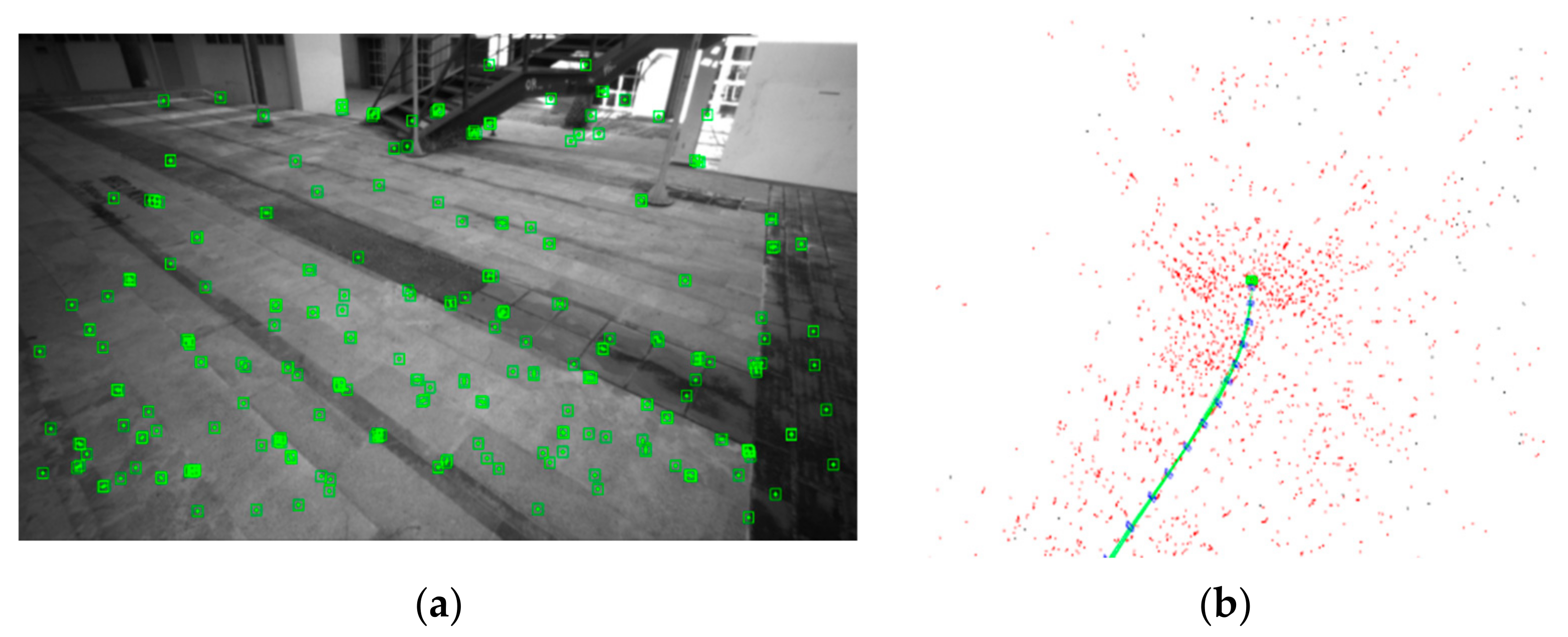

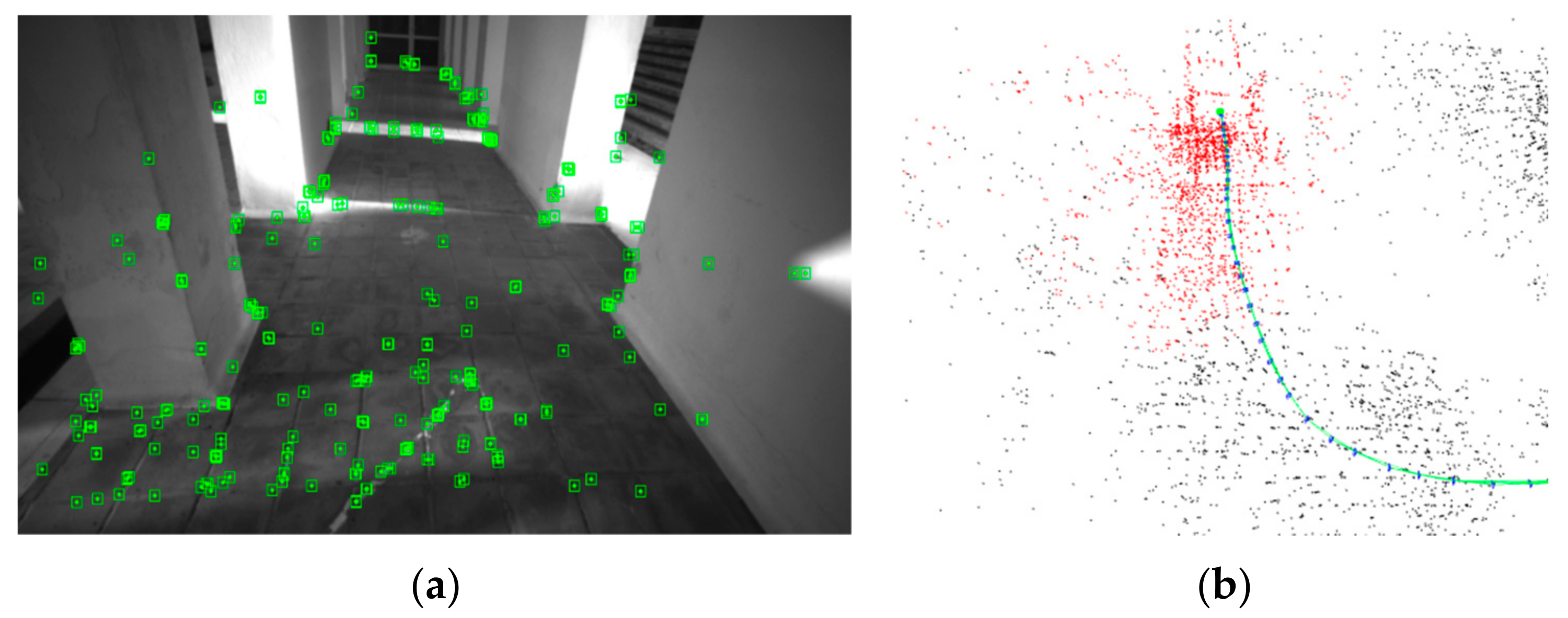
Figure 19.
Execution of vdio_slam in a GNSS-challenging corridor. (a) Detected features inside the corridor which are used by the SLAM algorithm for tracking. (b) The estimated trajectory up to the current position of the system in a local 3D map created by utilizing the ORB_SLAM2 algorithm. The red dots represent features of the local 3D space as point-cloud data that are currently detected, whereas the black ones represent all recorded features up to that moment.

Figure 20.
GNSS parameters recorded via the localization_core during a flight in a GNSS-challenging environment, along with their selected operational thresholds, of the first experiment.
Figure 20.
GNSS parameters recorded via the localization_core during a flight in a GNSS-challenging environment, along with their selected operational thresholds, of the first experiment.

Figure 21.
Overview of the operation of the thresholds, presented in Boolean logic, of the first experiment. The top figure indicates the regions where the number of satellites value, as well as its drop rate, contributed to producing a GNSS_WARNING state. The middle figure indicates the regions where the pDOP value, as well as its increase, contributed to producing a GNSS_WARNING state. The bottom figure is the logic OR operation of the previous figures, which indicates when the system was inside a GNSS_WARNING state.

Figure 22.
The overall acquired localization output track of the first experiment. This figure indicates the regions where the GNSS-IMU subsystem was selected as the localization source (yellow), as well as the regions where the system handed over the localization task to the vdio_slam (blue).
Figure 22.
The overall acquired localization output track of the first experiment. This figure indicates the regions where the GNSS-IMU subsystem was selected as the localization source (yellow), as well as the regions where the system handed over the localization task to the vdio_slam (blue).

Figure 23.
GNSS parameters recorded via the localization_core during a flight in a GNSS-challenging environment, along with their selected operational thresholds, of the second experiment. The graph containing the pDOP rate is a zoomed-in version as the values were extremely far from the threshold at a magnitude of about 2000.

Figure 24.
Overview of the operation of the thresholds, presented in Boolean logic, of the second experiment. The top figure indicates the regions where the number of satellites value, as well as its drop rate, contributed in producing a GNSS_WARNING state. The middle figure indicates the regions where the pDOP value, as well as its increase, contributed to producing a GNSS_WARNING state. The bottom figure is the logic OR operation of the previous figures, which indicates when the system was inside a GNSS_WARNING state.

Figure 25.
The overall acquired localization output track for the second experiment. This figure indicates the regions where the GNSS-IMU subsystem was selected as the localization source (yellow), as well as the regions where the system handed over the localization task to the vdio_slam (blue).
Figure 25.
The overall acquired localization output track for the second experiment. This figure indicates the regions where the GNSS-IMU subsystem was selected as the localization source (yellow), as well as the regions where the system handed over the localization task to the vdio_slam (blue).


Table 1.
Comparison of the accuracy regarding the selected localization subsystems.
| Method | Error 2D | Error Height | Error 3D | |||
|---|---|---|---|---|---|---|
| Average (m) | Variance (m2) | Average (m) | Variance (m2) | Average (m) | Variance (m2) | |
| GNSS | 0.0129 | 0.0002 | 0.0066 | <0.00005 | 0.0157 | 0.0002 |
| Stereo SLAM | 0.2195 | 0.0202 | 0.0402 | 0.0010 | 0.2255 | 0.0200 |
| RGBD SLAM | 0.0866 | 0.0024 | 0.0124 | 0.0001 | 0.0885 | 0.0023 |
| RGBD, IMU SLAM (VDIO) | 0.0832 | 0.0054 | 0.0142 | 0.0001 | 0.0881 | 0.0048 |
Table 2.
Accuracy evaluation of the localization system of the first experiment, inside a GNSS-challenging environment.
Table 2.
Accuracy evaluation of the localization system of the first experiment, inside a GNSS-challenging environment.
| Error 2D | Error Height | Error 3D | |||
|---|---|---|---|---|---|
| Average (m) | Variance (m2) | Average (m) | Variance (m2) | Average (m) | Variance (m2) |
| 0.0747 | 0.0052 | 0.1154 | 0.0223 | 0.1491 | 0.0240 |
Table 3.
Accuracy evaluation of the localization system of the second experiment, inside a GNSS challenging environment.
Table 3.
Accuracy evaluation of the localization system of the second experiment, inside a GNSS challenging environment.
| Error 2D | Error Height | Error 3D | |||
|---|---|---|---|---|---|
| Average (m) | Variance (m2) | Average (m) | Variance (m2) | Average (m) | Variance (m2) |
| 0.0747 | 0.0052 | 0.1154 | 0.0223 | 0.1491 | 0.0240 |
Publisher’s Note: MDPI stays neutral with regard to jurisdictional claims in published maps and institutional affiliations. |
© 2022 by the authors. Licensee MDPI, Basel, Switzerland. This article is an open access article distributed under the terms and conditions of the Creative Commons Attribution (CC BY) license (https://creativecommons.org/licenses/by/4.0/).
Share and Cite
MDPI and ACS Style
Antonopoulos, A.; Lagoudakis, M.G.; Partsinevelos, P. A ROS Multi-Tier UAV Localization Module Based on GNSS, Inertial and Visual-Depth Data. Drones 2022, 6, 135. https://0-doi-org.brum.beds.ac.uk/10.3390/drones6060135
AMA Style
Antonopoulos A, Lagoudakis MG, Partsinevelos P. A ROS Multi-Tier UAV Localization Module Based on GNSS, Inertial and Visual-Depth Data. Drones. 2022; 6(6):135. https://0-doi-org.brum.beds.ac.uk/10.3390/drones6060135
Chicago/Turabian StyleAntonopoulos, Angelos, Michail G. Lagoudakis, and Panagiotis Partsinevelos. 2022. "A ROS Multi-Tier UAV Localization Module Based on GNSS, Inertial and Visual-Depth Data" Drones 6, no. 6: 135. https://0-doi-org.brum.beds.ac.uk/10.3390/drones6060135