High-Precision Seedling Detection Model Based on Multi-Activation Layer and Depth-Separable Convolution Using Images Acquired by Drones

Abstract

Crop seedling detection is an important task in the seedling stage of crops in fine agriculture. In this paper, we propose a high-precision lightweight object detection network model based on a multi-activation layer and depth-separable convolution module to detect crop seedlings, aiming to improve the accuracy of traditional artificial intelligence methods. Due to the insufficient dataset, various image enhancement methods are used in this paper. The dataset in this paper was collected from Shahe Town, Laizhou City, Yantai City, Shandong Province, China. Experimental results on this dataset show that the proposed method can effectively improve the seedling detection accuracy, with the F1 score and mAP reaching 0.95 and 0.89, respectively, which are the best values among the compared models. In order to verify the generalization performance of the model, we also conducted a validation on the maize seedling dataset, and experimental results verified the generalization performance of the model. In order to apply the proposed method to real agricultural scenarios, we encapsulated the proposed model in a Jetson logic board and built a smart hardware that can quickly detect seedlings.

1. Introduction

The rapid and accurate identification of plant seedlings in the natural environment is essential to achieving precise pesticide spraying [1]. However, the accurate identification of plant seedlings is affected by the complex background environment such as light changes, weather, weeds, and terrain [2,3,4]. As an important data source for precision agriculture, drone remote sensing images can be used to protect crops, measure the quality of crops, and realize plant seedling identification [5,6,7,8,9,10].

Seedling identification plays an irreplaceable role in the cultivation and production of wheat. By identifying wheat seedlings, the location and extent of weed distribution can be inferred, and weeds can be managed precisely. Weeds affect the yield and quality of crops in agricultural production, mainly because weeds compete with crops for sunlight, oxygen, nutrients, and space, which hinder crop growth [3]. At the same time, weeds are also intermediate hosts for many pathogens and pests, leading to pests and diseases. In addition, some weed seeds and pollen may carry toxins, which can threaten the health of humans and animals.

Drones are now widely used in agricultural production, and some results have been achieved in yield estimation. The techniques of image analysis and height and phenotype in yield estimation have commonality in wheat seedling identification [11,12]. Meanwhile, drones have important applications in plant growth, disease identification, and nutrient level measurement. Among them, nutrient level measurement can effectively distinguish wheat seedlings from weeds in the actual environment, which has a positive effect on wheat seedling identification; the image classification in disease identification also has a certain correlation with wheat seedling identification; meanwhile, wheat seedling identification can be widely applied in agricultural production, where one of the important aspects of plant growth is weed elimination.

Flores et al. proposed an agave counting method based on aerial data collected by drones and computer image processing. It improved the detection performance through a Convolutional Neural Network (CNN) and achieved an F1 score of 0.96 compared to 0.57 for the algorithm of Hear [13]. Csillik et al. used a CNN to detect citrus and other trees with the help of drone images and then classified them using superpixels derived from Simple Linear Iterative Clustering (SLIC). The process performed well in agricultural environments with multiple targets, multiple ages of trees, and multiple sizes of trees, achieving an overall accuracy of 96.24%, a positive predicted value of 94.59%, and a sensitivity of 97.94% [14]. You Only Look Once (YOLO) v5, proposed by Chaschatzis et al., has performed well in detecting infected leaves and infected branches on perennial-fruit-based crops such as sweet cherries [15].

Combining three characteristic selection methods and two classification groups, Garzon-Lopez et al. used hyperspectral data, Support Vector Machine (SVM), and Random Forest (RF) classifiers to test their ability to detect five typical Paramo species with diverse growth forms. With the help of Red Green Blue (RGB) images, they classified 21 species with a precision of over 97%. In terms of hyperspectral imaging, the model established using RF or SVM classifiers combined with binary group formation methods and sequential floating selection features had the highest accuracy (89%). The results showed that the Palamo species map could be accurately drawn using RGB and hyperspectral images [16].

The image recognition algorithm by Jooste, J. et al. focused on extracting information from height conditions and found that the structure of the network played a key role and the choice of adding height information directly to the fourth image channel did not show any improvement [17]. Chen, Y. et al. proposed a combined multi-feature fusion and SVM approach for detecting weeds in wheat and rice, which can be used accurately for classification and can enable precise application of fertilizer to the land, which has achieved good results in the relevant dataset [18]. Jian, M. et al. proposed a local color contrast model that can separate objects from the background and can capture the main features of the objects to be classified, which greatly reduces the computational cost [19].

From the above analysis, it is easy to see that although drones have been used in many agricultural applications, there are still several areas for improvement:

• The extent to which practical measurement techniques can be applied in real agricultural scenarios needs to be improved because of the problem of portability.
• There is still room for further improvement in model performance [13,20].
• The results of encapsulating models into hardware so that theoretical innovations can be directly deployed in agricultural production are still scarce.

Therefore, this paper proposes the Generative Adversarial Network (GANLite) seedling detection network based on multi-activation layer and depth-separable convolution. The goal is to reduce the number of convolutional network parameters and to improve the inference speed, so that it can be deployed in edge computing devices that can be mounted on drones. The main contributions are as follows:

• We added noise to the feature map using the generative network to improve the robustness of the model.
• We modified a one-stage object detection network by using deep separable convolution, which significantly reduced the number of model parameters, lowered the model complexity, and improved the model operation efficiency, while maintaining the model performance.
• We propose a multi-activation layer instead of the existing activation function layer to improve the model’s ability to fit complex functions.

2. Related Work

With the development of deep learning, the target detection technology based on deep learning has made great progress, but the detection of small targets faces great challenges and difficulties due to the small number of pixels, which makes it difficult to extract enough information.

The detection task in this paper is a target detection task for small targets. Compared with the detection of large and medium-sized targets, there is still a big gap in the detection performance of small targets. Deep-learning-based target detection methods can be divided into two categories. One is the two-stage target detection method. In this method, candidate regions are first generated, and then, the candidate regions are classified and regressed, such as Faster R-CNN [21]. The other is a single-stage target detection method, which regresses the class and coordinates of the object directly from the image without generating candidate frames. The usual methods are YOLO [22,23,24,25,26], SSD (single shot detector) [27], etc.

Since the two-stage model can be regarded as the splicing of the proposed bounding box generation and one-stage model to some extent, the following is an example of a Faster R-CNN network to analyze the technical framework of target detection network.

2.1. Two-Stage Objection Detection: Faster R-CNN

2.1.1. Shared Convolutional Layer

The shared convolutional layer performs the initial feature extraction of the input feature map, and the extracted feature maps are used for sharing between Region Proposal Networks (RPNs) and FastR-CNN. FastR-CNN often uses Visual Geometry Group Network (VGGNet 16) [28] as a shared convolutional network to map the original input feature map into a 512-dimensional feature map and reduce the training parameters for network back-propagation.

2.1.2. RPN Network

The RPN structure’s input is a convolutional feature map, and k anchor frames of $3\times 3$ are generated by centering each pixel in the low-dimensional feature map of size $w\times h$, so that a total of $w\times h\times k$ anchor frames are generated for each feature map. The regression analysis and classification of the generated anchor frames are performed by the regression and classification layers connected behind. The regression layer selects the target suggestion regions that may contain targets, and the classification layer determines the score of each target suggestion region; finally, the generated results are parameterized. The target suggestion regions with high scores are input to the region of the interest pooling layer of FastR-CNN.

The RPN network is trained end-to-end. During the training, the network calculates the loss function value of each layer by back-propagation and continuously updates the network weights according to the value of the loss function. The smaller the value of the loss function, the better the robustness of the model. The loss function is shown in Equation (1).

$$L(p_i,t_i)=\frac{1}{N_{cls}}\sum _i{L}_{cls}(p_i,p_i^{\ast })+\lambda \times \frac{1}{N_{reg}}\sum _i{p}_i^{\ast }g{L}_{reg}(t_i,t_i^{\ast })$$

(1)

where i denotes the value of the anchor box retrieval in the small batch graph; $p_i$ denotes the probability that the anchor frame contains the target; $p_i^{\ast }$ takes 1 if the anchor frame extracts the target correctly; otherwise, it is 0; $t_i$ is the four parameterized coordinates of the predicted target frame; $t_i^{\ast }$ is the parameterized coordinates of the actual target frame; $N_{cls}$ denotes the number of all samples in a mini-batch; $N_{reg}$ denotes the number of anchor positions, about 2400; $L_{cls}\left(\right)$ and $L_{reg}\left(\right)$ are the classification loss function and the regression loss function, respectively, as shown in Equations (2) and (3).

$$L_{cls}(p_i,p_i^{\ast })=-log[p_i{p}_i^{\ast }+(1-p_i)(1-p_i^{\ast })]$$

(2)

$$L_{reg}(t_i,t_i^{\ast })=\left\{\begin{array}{c}\hfill 0.5{(t_i-t_i^{\ast })}^2,if|t_i-t_i^{\ast }|<1\\ \hfill |t_i-t_i^{\ast }|-0.5,else\end{array}\right.$$

(3)

The border regression of the RPN network is a linear regression operation between the predicted border and the actual border to obtain the predicted border closest to the actual border, where the coordinates of the border are calculated as follows:

$$t_x=\frac{(x-x_a)}{w_a},t_y=\frac{(y-y_a)}{h_a}$$

(4)

$$t_w=log\left(\frac{w}{w_a}\right),t_h=log\left(\frac{h}{h_a}\right)$$

(5)

$$t_x^{\ast }=\frac{(x^{\ast }-x_a)}{w_a},t_y^{\ast }=\frac{(y^{\ast }-y_a)}{h_a}$$

(6)

$$t_w^{\ast }=log\left(\frac{w^{\ast }}{w_a}\right),t_h^{\ast }=log\left(\frac{h^{\ast }}{h_a}\right)$$

(7)

where $(x,y)$ are the center coordinates of the predicted border, w and h are its width and height, $(x^{\ast },y^{\ast })$ and $(x_a,x_b)$ are the center coordinates of the real border and anchor frame, respectively, and $w^{\ast }$, $w_a$, $h^{\ast }$, and $h_a$ are its width and height.

The RPN inputs the generated proposed regions into the ROI pooling layer of Faster R-CNN to lower the feature map resolution, reduce the training parameters, and speed up the convergence of the neural network. The parameters are then fed into two fully connected layers. Finally, the target frame is selected using regression analysis and classified using a Softmax classifier, which outputs the predicted target frame and the probability that the target frame may be the correct target.

3. Materials

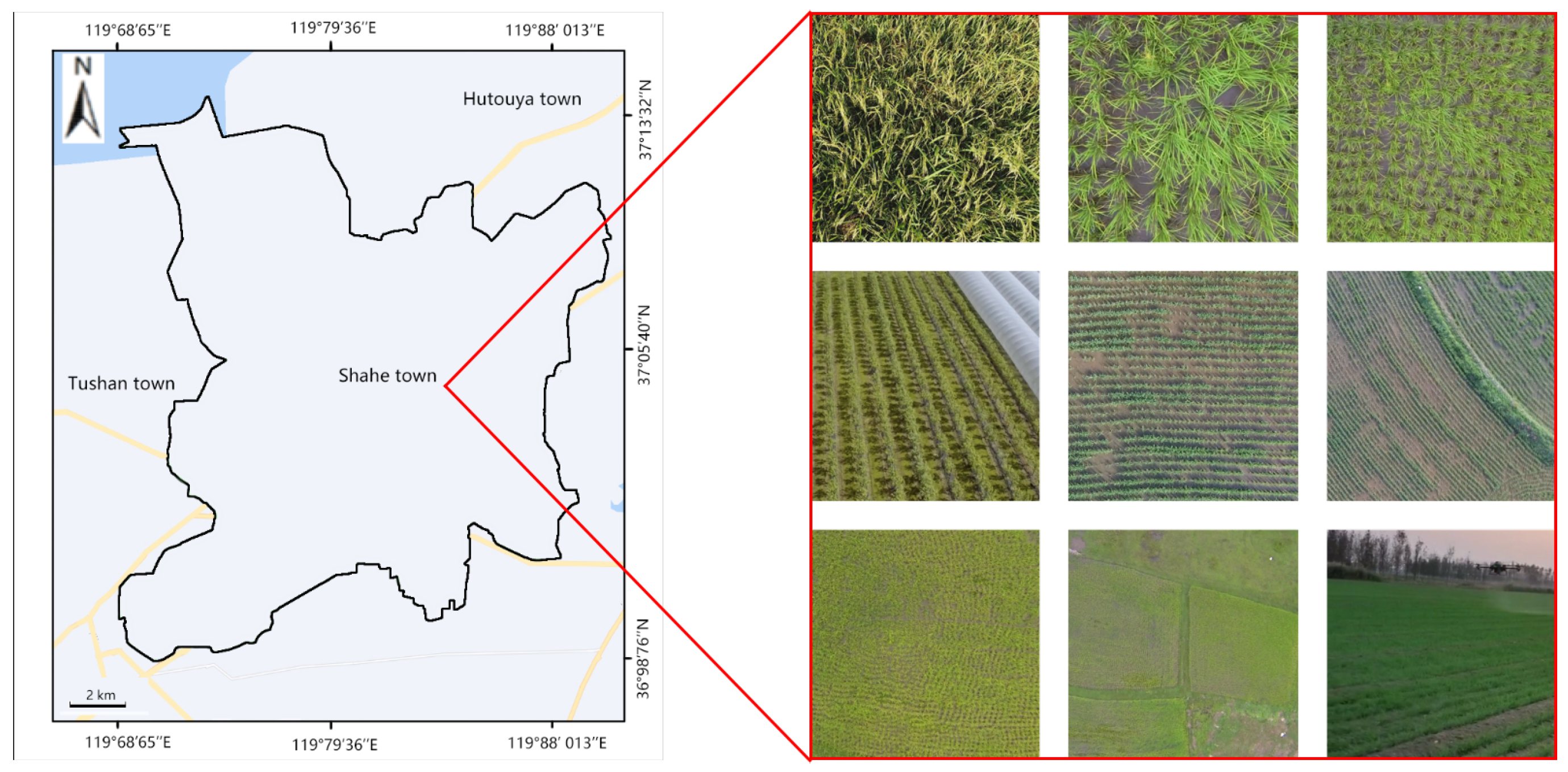
3.1. Image Acquisition

The images of plant seedlings were collected in Shahe Town, Laizhou City, Yantai City, Shandong Province, China, at 09:00–14:00 and 16:00–18:00 on 8 April 2022. The crop was in the seedling stage at the time of data collection. The collected images are shown in Figure 1.

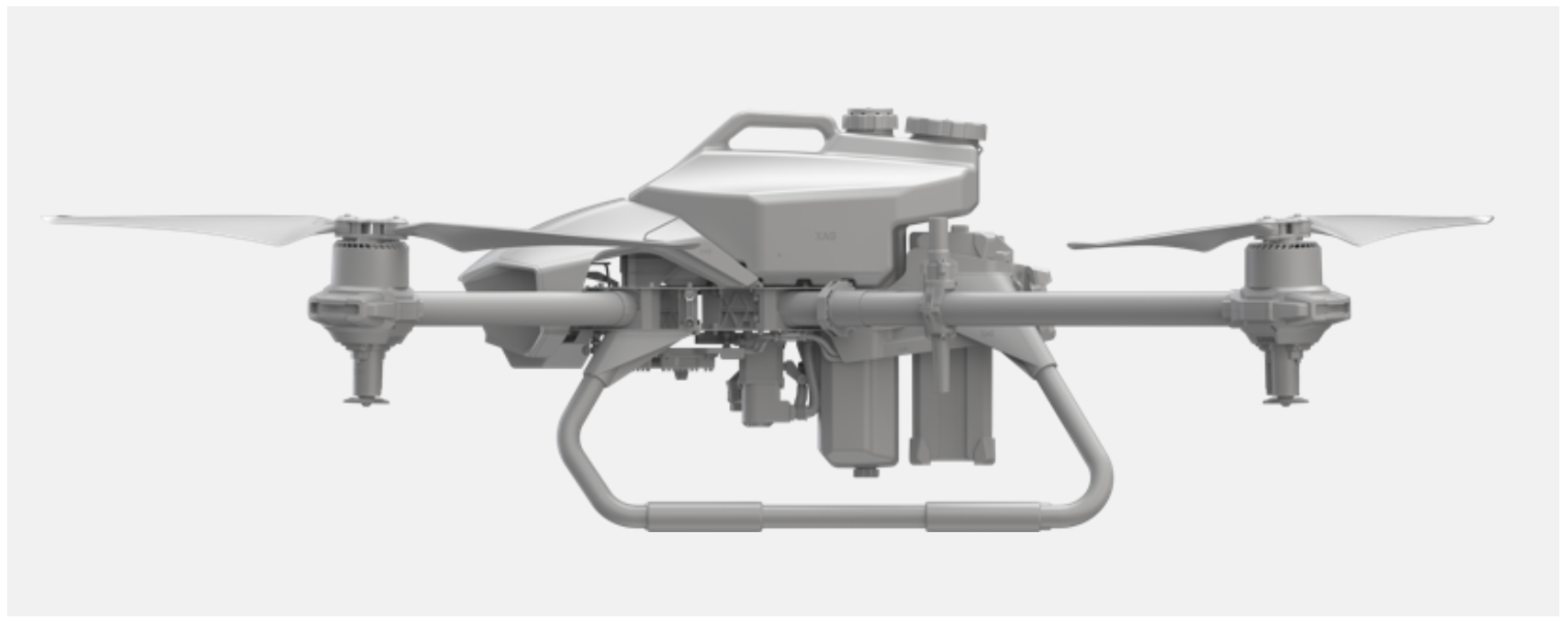
In this paper, the acquisition device is a Polaris xp2020 drone, as shown in Figure 2. It is a multi-rotor system with four motors (quadrotor), an asymmetric motor axis distance of 1680 mm, a maximum thrust-to-weight ratio of 1.9, and a maximum operational flight speed of 12 m/s, and it is powered by a lithium polymer B13860S intelligent battery with an operational endurance of 10 min. Its weight is 19.27 kg. It has a wingspan of 20 cm and a load ratio of 0.43.

The drone is equipped with a Canon 5D camera (stabilized by a tripod). This camera acquires solid color images at 8 bit resolution. The acquisition is performed automatically at a predetermined cadence during flight preparation. The system uses autonomous ultrasonic sensor flight technology to reduce the risk of accidents. The system includes a ground control radio connected to a smartphone with a range of 5 km (without obstacles) under normal conditions.

3.2. Image Normalization and Labeling

After compressing and batch naming the images, the input image resolution was adjusted to $1920\times 1080$. Labelme, a professional labeling software, was used to label the largest outer rectangle of the target plant seedlings with a green box. The labeling file format was saved as a .xml file, which contained the location and pixel information of the labeled features.

In this paper, we normalized the images before training the model to adjust the size of the feature values to a similar range. This is because, without normalization, the gradient values will be larger when the feature values are larger and smaller when the feature values are smaller. When the model is back-propagated, the gradient value update is the same as the learning rate; when the learning rate is small, the gradient value is small, which will lead to a slow update; when the learning rate is large, the gradient value is large, which will lead to a model that does not easily converge. In order to make the model training converge smoothly, a normalization operation is performed on the image to adjust the feature values of different dimensions to a similar range, and then, a uniform learning rate can be used to accelerate the model training. The specific formula is as follows:

$$output=\frac{input-min\left(input\right)}{max\left(input\right)-min\left(input\right)}$$

(8)

where $output$ is the image pixel value output, $input$ is the image pixel value input, $max$ and $min$ are the maximum and minimum pixel values, and the pixel values are adjusted to the $(0,1)$ interval after normalization.

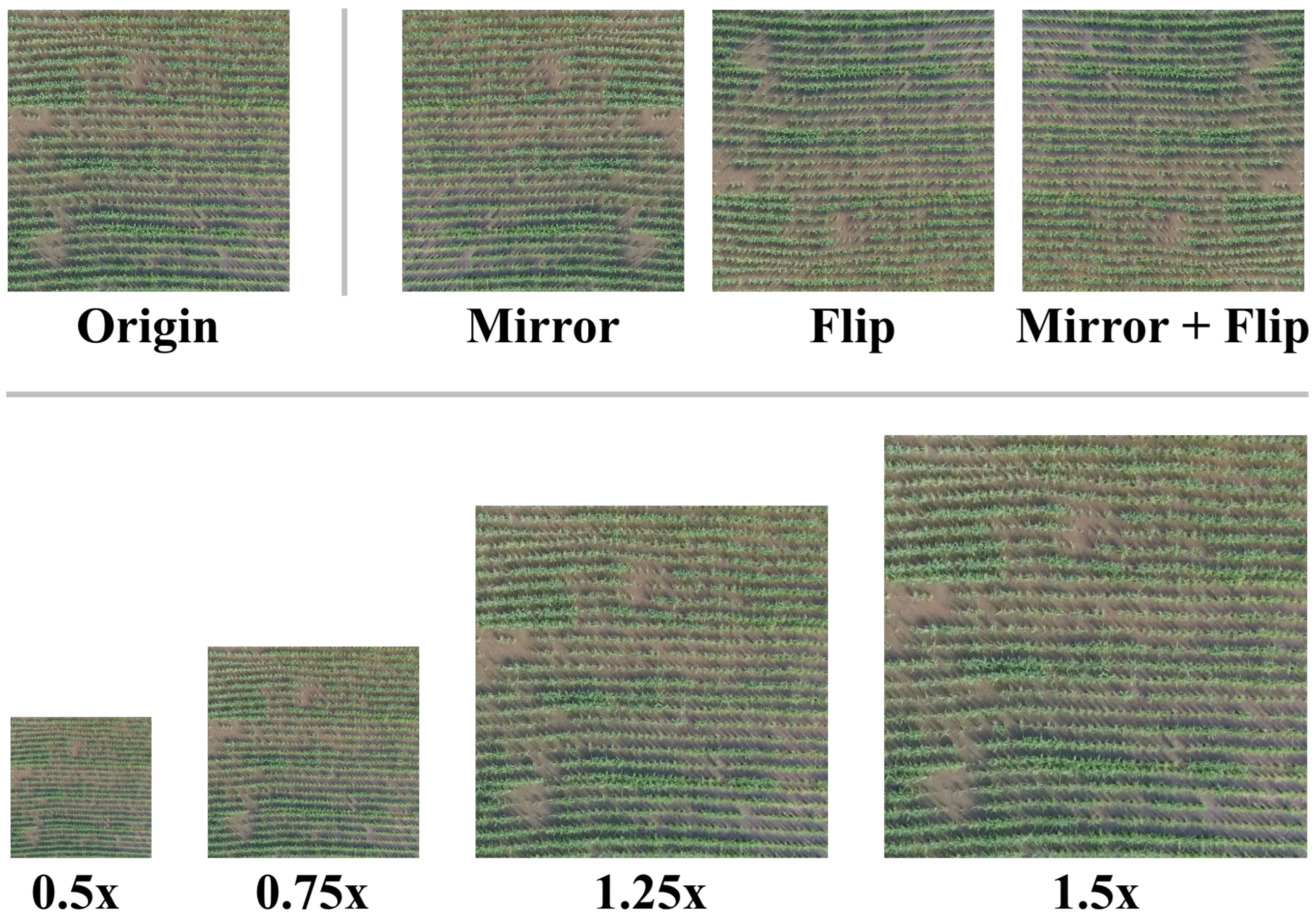
3.3. Dataset Augmentation

Data augmentation is applied to the data to cope with the diverse environment of the field and increase the robustness and generalization ability of the plant seedling recognition model. In terms of expanding the amount of data for training, the main methods of data augmentation are flipping, rotating, scaling, cropping, panning, etc. Geometric deformation is used to expand the number of sample sets to avoid the distortion of model parameters’ extraction or model overfitting due to the sample size or scale problems. In terms of noise suppression, data enhancement methods mainly include adding noise, changing the image brightness or contrast, etc., which simulate the effect of a complex noise interference and lighting environment by changing the visual effect of the image and then suppressing the problem of the low accuracy of the training model caused by poor quality, such as image noise and image blur.

In this paper, the data expansion of the training set and validation set was carried out in the above two categories. The constructed datasets of plant seedling images are shown in Figure 3 and

Table 1. Dataset distribution details.

Dataset	Dataset Augmentation Method	Number of Images
Training set	Origin	2100
	Brightness and hue	4200
	Flip and mirror	2100
	Scale	2100
Validation set	Origin	600
	Brightness and hue	1200
	Flip and mirror	600
	Scale	600
Test set	Origin	300

.

The training set, validation set, and test set were divided into a 7:2:1 ratio. Then, we expanded the divided training set and validation set. There were 10,500 images in the training set, 3000 images in the validation set, and 300 images in the test set after the expansion.

4. Proposed Model

As described in Section 2, the mainstream two-stage object detection model, Faster R-CNN, has shown excellent detection results on the Microsoft Common Objects in Context (MS COCO) [29] and Pascal Visual Object Classes (VOC) [30] datasets. However, Faster R-CNN does not apply to the dataset used in this paper.

As mentioned in Section 3, the actual agricultural dataset used in this paper is characterized by a small object, high density, and variable illumination. Faster R-CNN is not optimized for small objects. There are high-density small object detection scenarios in practical applications. The general approaches to solving the small object detection problem include: increasing the resolution of the input image, which increases the computational complexity, and multi-scale feature representation, which makes the results uncontrollable. Currently, the mainstream detection networks contain the Feature Pyramid Network (FPN) [31]. After the features are extracted from the backbone network, the FPN contains the fusion of the neck network with the deep and shallow feature maps. This structure improves the network’s ability to detect objects at different scales. However, it also makes the network complex and has the possibility of overfitting. Furthermore, as the network becomes more complex and the model parameters become more numerous, deploying it in lightweight hardware becomes increasingly tricky.

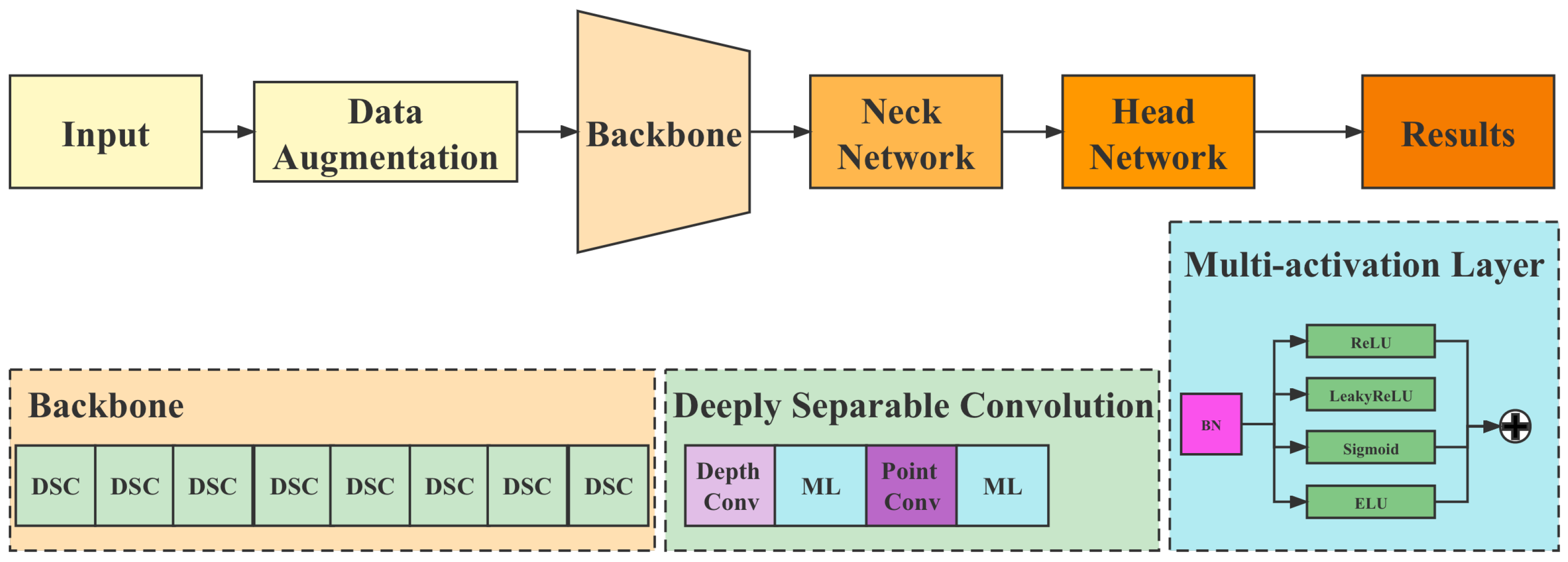
Regarding the above issues, this paper proposes a GANLite detection network based on the Generative Adversarial Network (GAN) model, a multi-activation layer, and a lightweight network. Compared with the mainstream object detection models, including the one-stage and the two-stage ones, the main innovations of GANLite detection are:

• We added noise to the feature map using the generative network to improve the robustness of the model. Figure 4 compares the original feature map with the feature map obtained by adding noise to the GAN model.
• We modified a one-stage object detection network by using deep separable convolution, which significantly reduces the number of model parameters, lowers the model complexity, and improves the model operation efficiency, while maintaining model performance. The specific implementation is in Section 4.2.
• We propose a multi-activation layer instead of the existing activation function layer to improve the model’s ability to fit complex functions.

The structure of GANLite detection is shown in Figure 5.

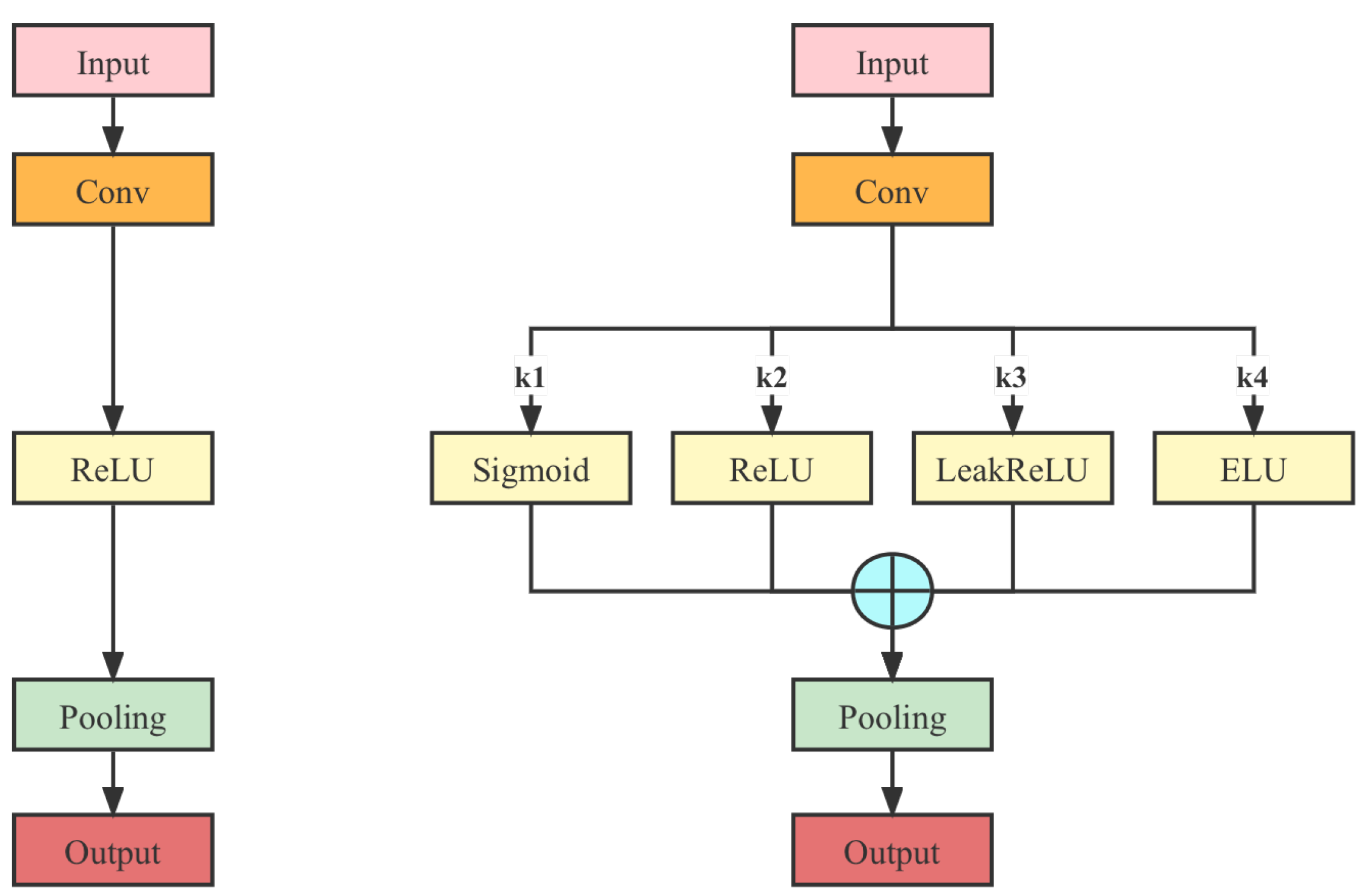
4.1. Multi-Activation Layer

There are only tandem activation function layers in the existing network structure, mainly the Rectified Linear Unit (ReLU) and LeakyReLU, between the layers. In this paper, we propose a multi-activation layer, which transforms the tandem activation function layer into a multi-activation function layer with coefficients $k_n$ in front of each base activation function and ensures that ${\sum }_{i=1}^n{k}_i=1$. Therefore, the effect of integrating multiple CNN models can be simulated through the multi-activation layer, as shown in Figure 6.

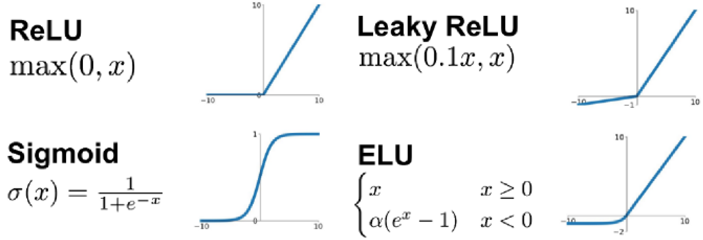
Specifically, there are several types of base activation functions that can form a multi-activation layer, including ReLU, LeakyReLU, Exponential Linear Unit (ELU), and Sigmoid, as shown in Figure 7.

Since the coefficients k in front of each activation function are adjustable, the model can be fit to different cases by tuning the values of these coefficients. For example, when $k_3=0$ and the other coefficients are 0, the module is equivalent to a single LeakyReLU layer. The detection performance of the model obtained by combining different values of the coefficients k is compared in Section 7.2.

4.2. Lightweight Detection Network

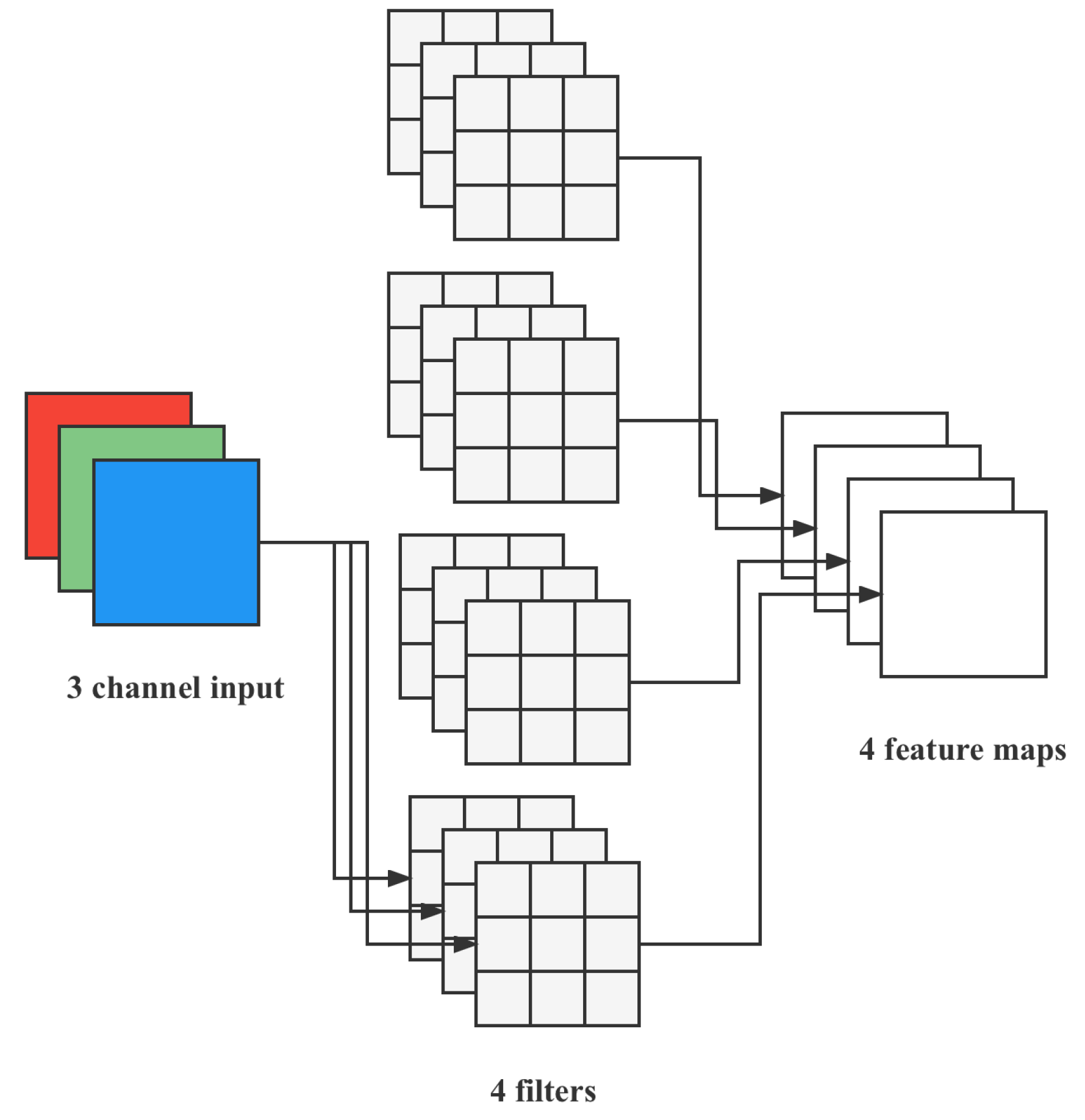
4.2.1. General Convolution Operation

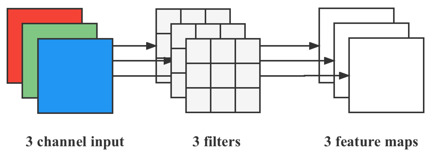
For a $5\times 5$, three-channel (shape of $5\times 5\times 3$) image, after the convolution layer of the $3\times 3$ kernel (assuming the number of output channels is 4 and the kernel shape is $3\times 3\times 3\times 4$), 4 feature maps are finally output. If there is same padding, then the size of the input layer is the same, $5\times 5$; if not, the size becomes $3\times 3$.

From Figure 8, we can see that the convolutional layer has 4 filters, and each filter contains 3 kernels, while the size of each kernel is $3\times 3$. Therefore, the number of parameters of the convolutional layer can be calculated by the following formula: $N_{std}=4\times 3\times 3\times 3=108$.

4.2.2. Deeply Separable Convolution

One kernel of depth convolution is responsible for one channel, and one channel is convolved by only one kernel. A $5\times 5$, three-channel color input image (shape is $5\times 5\times 3$) needs to go through the first convolution operation of depth convolution, and depth convolution is completely performed in a two-dimensional plane. The number of kernels is the same as the number of channels in the previous layer (channels and kernels correspond one-to-one). Therefore, a three-channel image is computed, and three feature maps are generated ($5\times 5$ if there is the same padding), as shown in Figure 9.

One filter contains only one kernel of size $3\times 3$, and the number of parameters in the convolution part is calculated by the following formula: $N_{depthwise}=3\times 3\times 3=27$. The number of feature maps after depth convolution is the same as the number of channels in the input layer, but it is not possible to extend the feature map. Moreover, this operation performs the convolution operation on each channel of the input layer independently and does not effectively utilize the feature information of different channels at the same spatial position. Therefore, pointwise convolution is needed to combine these feature maps to generate a new feature map.

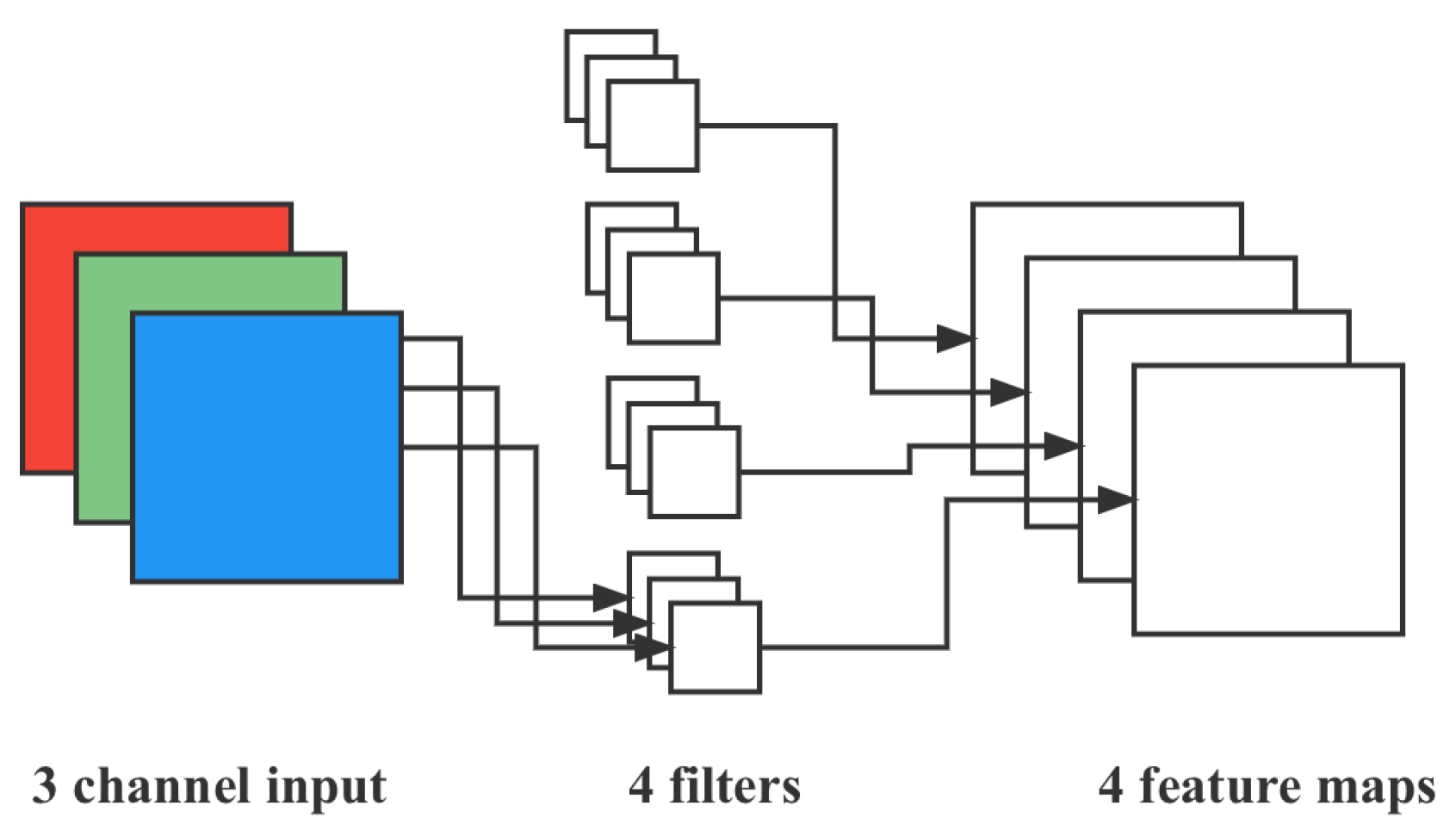
The operation of pointwise convolution is very similar to the conventional operation. The size of its kernel is $1\times 1\times M$, and M is the number of channels in the previous layer. Therefore, the convolution operation here will perform a weighted combination of the previous map in the depth direction to generate a new feature map. The number of output feature maps is the same as the number of kernels.

From Figure 10, we can see that the number of parameters involved in the convolution step can be calculated as $N_{pointwise}=1\times 1\times 3\times 4=12$ since the $1\times 1$ convolution method is used.

4.2.3. Lightweight Design of Object Detection Network

From the above discussion, the number of parameters of the regular convolution is: $N_{std}=4\times 3\times 3\times 3=108$. The parameters of the separable convolution are obtained by adding two parts: $N_{depthwise}=3\times 3\times 3=27$, $N_{pointwise}=1\times 1\times 3\times 4=12$, $N_{separable}=N_{depthwise}+N_{pointwise}=39$.

For the same input and 4 feature maps obtained, the number of parameters of separable convolution is about $\frac{1}{3}$ of that of conventional convolution. Therefore, the number of layers of the neural network can be deeper with the same number of parameters.

By replacing all the convolutional layers in the one-stage network with deeply separable convolutions, we reduce the number of parameters to one-third of the original one, which significantly improves the inference speed of the network, as seen in Section 6.

5. Experiments

5.1. Experiment Settings

The test device is a desktop computer with a Core i9-10900k CPU and Nvidia RTX3080 GPU. In the training process, the experiments were run on Ubuntu 20.14, using the Python programming language, and the model implementation was based on the PyTorch framework; the number of learning rounds was set to 150, and the network was optimized using the stochastic gradient descent algorithm, where the initial learning rate was $1\times {10}^{-5}$.

5.2. Model Evaluation Metrics

In order to validate the effectiveness of the model for field plant seedling detection, Recall (R) and Precision (P) were used as the evaluation metrics. The evaluation parameters used for target detection are shown in

Table 2. Matrix of classification indicators.

	Contained	Uncontained
Detected	TP	FP
Undetected	FN	TN

.

Among them, TP indicates the number of seedlings detected as valid optimistic targets and included; FP indicates the number of seedlings detected as false optimistic targets and not included; FN indicates the number of seedling false-negative targets not detected and included; TN indicates the number of seedlings that are proper targets not detected and not included.

Precision (P) represents the proportion of detected targets contained in images of detected targets and is defined by the formula:

$$P=\frac{TP}{TP+FP}$$

(9)

Recall (R) represents the proportion of images containing successfully detected targets and is defined by the formula:

$$R=\frac{TP}{TP+FN}$$

(10)

The F1 balances precision and recall and is defined by the formula:

$$F1=\frac{2\times P\times R}{P+R}$$

(11)

The AP calculation is slightly different for different datasets, but the overall idea is a differential calculation of the area of the PR curve. voc2007’s calculation smooths the curve first and takes the largest precision value to the right of each point to form a straight line. coco uses 101 interpolation points to calculate the AP, which is a more detailed consideration. Furthermore, it also calculates the AP for different Intersection over Union (IoU) thresholds; the first line of the result below is the IoU threshold within (0.5–0.95), each 0.05 to take a value to calculate the AP. The AP value calculation is only for one category. After obtaining the AP, the calculation of the mAP becomes very simple, which is calculating the AP for all categories and then taking the average. The calculation formula is as follows:

$$mAP=\frac{{\sum }_{i=1}^{num\_class}A{P}_i}{num\_class}$$

(12)

F1, mIoU, and network detection speed were selected as evaluation metrics.

6. Results

6.1. Validation Results

Table 3. Comparison of various models and ours.

Method	F1	mAP	FPS
Faster R-CNN	0.83	0.69	31.9
Mask R-CNN	0.87	0.76	29.4
EfficientDet	0.93	0.72	33.2
YOLO v3	0.92	0.77	52.1
YOLO v4	0.91	0.77	47.5
YOLO v5	0.93	0.81	53.8
SSD	0.89	0.79	45.6
ours	0.95	0.89	87.3

shows the results of all the tests performed in this paper. The comparison networks include the mainstream one-stage networks, YOLO, SSD, and EfficientDet [32], and the mainstream two-stage networks, Mask R-CNN [33] and Faster R-CNN. The best results are marked in bold in the table.

From Table 3, we can see that the proposed model has the fastest inference speed, with an Frames Per Second (FPS) speed of 87.3, and the only network that compares with our model is YOLO, whose FPS speed is only 53.8. The F1 and mAP of Faster R-CNN are 0.83 and 0.69, and its performance is the worst among all models. The F1 and mAP of YOLO v5 outperform Faster R-CNN, Mask R-CNN, and SDD with values of 0.93 and 0.81, respectively, and YOLO v5 has the best performance even among all YOLO series of networks. Although EfficientDet outperforms the other compared networks in the F1 metric, its mAP metric only outperforms Faster R-CNN. this may be due to the presence of EfficientDet’s attention extraction module, which makes its F1 metric high. Overall, YOLO v3 and YOLO v5 are the best two models among the compared models. Our model achieves 0.95 and 0.89 in F1 and mAP, respectively, which are higher than YOLO v5 and EfficientDet and all the compared models. Moreover, our model has the fastest inference speed among all the models.

6.2. Detection Results

For further comparison, several images were extracted from the seedling images in the test set. These images show as many detection scenarios as possible in the dataset, such as images with multiple lighting conditions, images collected at different flight altitudes, and scenarios where the seedlings in the images are too small and too sparse. Figure 11 shows the detection results for different object detection networks, where the red box is the ground truth and the green box is the predicted bounding box generated by the algorithm.

From Figure 11, we can see that Faster-RCNN performs very poorly on these four images, while EfficientDet, SSD, and YOLO perform relatively well and can detect the lesions accurately. However, when the detected seedlings are too small, i.e., the flight altitude is too high, the performance of all models degrades, and some of them even have some unlabeled detected objects. This situation may be related to the attention extraction module in these networks.

As can be seen from the experimental result plots, our model outperforms the other models, although there is still room for improvement. That is true even when detecting high-density images, i.e., containing a large number of seedlings. Considering that our model uses fewer parameters and has lower complexity, this offers the possibility of deploying the algorithm on low-cost hardware.

7. Discussion

7.1. Validation on GAN Module

This paper uses pre-GAN in the backbone, and this GAN module generates an attention mask to enhance the model’s robustness. Therefore, different GAN models were implemented in this paper, including WGAN [34,35], SAGAN [36], and SPA-GAN. Several ablation experiments were conducted, and the experimental results are shown in

Table 4. Results of different implements of GAN module.

Method	F1	mIoU	FPS
No GAN (baseline)	0.91	0.83	101.2
WGAN	0.95	0.89	87.3
SAGAN	0.95	0.87	85.4
SPA-GAN	0.92	0.83	77.8

.

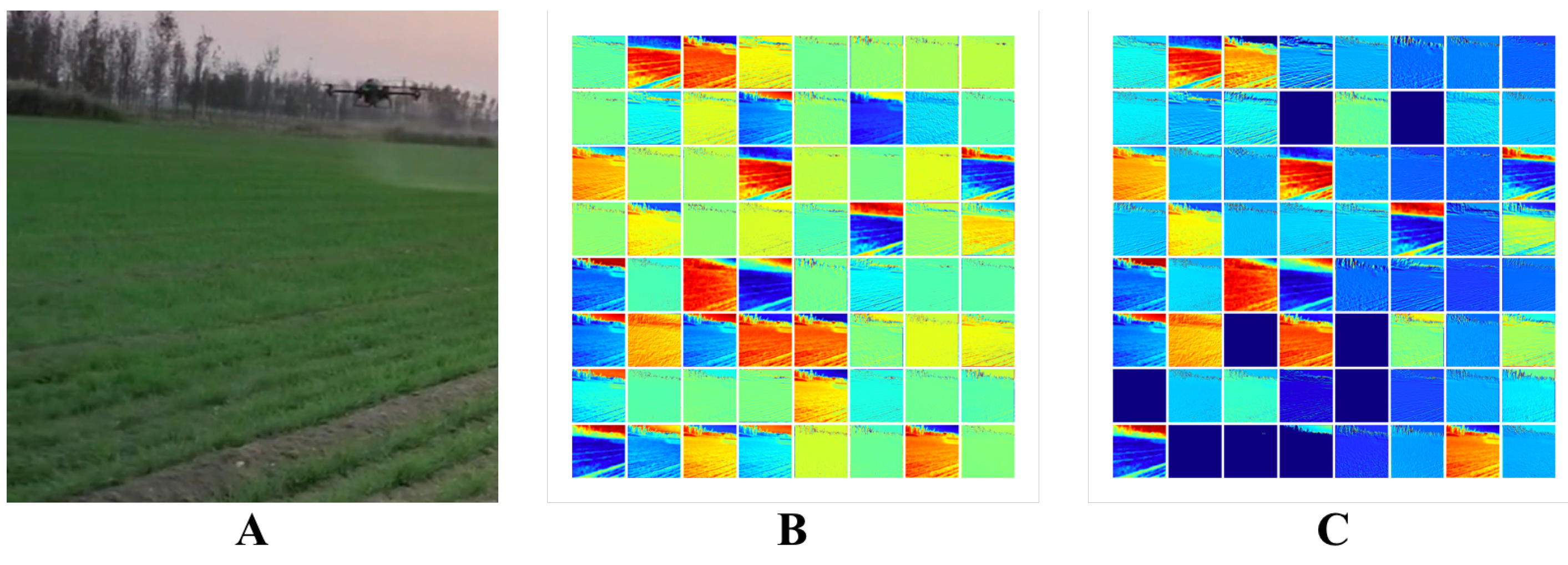
Table 4 reflects that using WGAN and SPA-GAN to implement the GAN module, respectively, can optimize the model performance significantly. As a comparison, WGAN is better than SPS-GAN in the choice. By comparing the baseline model, it is apparent that the GAN module, regardless of the implementation approaches, can significantly improve the model’s performance by 6% in terms of the $mIoU$ parameter. Furthermore, we tried to visualize the noise mask, as shown in Figure 4C.

7.2. Validation on Multi-Activation Layer

This section discusses the effect of different values of coefficients $k_i$ in the multi-activation layer on the model performance, and experimental results are shown in

Table 5. Top-1 and top-3 accuracy of different models.

${\mathit{k}}_1$ (ReLU)	${\mathit{k}}_2$ (LeakyReLU)	${\mathit{k}}_3$ (Sigmoid)	${\mathit{k}}_4$ (ELU)	F1	mIoU
1.0	0.0	0.0	0.0	0.88	0.79
0.0	1.0	0.0	0.0	0.92	0.85
0.0	0.0	1.0	0.0	0.63	0.51
0.0	0.0	0.0	1.0	0.88	0.83
0.25	0.25	0.25	0.25	0.85	0.77
0.70	0.10	0.10	0.10	0.88	0.79
0.10	0.70	0.10	0.10	0.93	0.85
0.10	0.10	0.70	0.10	0.71	0.65
0.10	0.10	0.10	0.70	0.95	0.89

.

The experimental results show that the effect of the multi-activation layer depends mainly on the coefficients k before different activation functions. When k is uniformly taken as 0.25 or Sigmoid dominates, the model’s performance is severely degraded; when $k_1,k_2,k_3,k_4$ are taken as 0.1, 0.1, 0.1, 0.7, respectively, the ELU function dominates, and the model’s accuracy improvement is most apparent.

7.3. Ablation Experiment of Data Augmentation

To verify the effectiveness of the various pre-processing methods proposed in Section 3.3, the ablation experiments were performed on our model. The experimental results are shown in

Table 6. Ablation experiment result of different pre-processing methods (in %).

Augmentation Method	mIoU	mAP
None	0.90	0.81
Brightness and hue	0.93	0.85
Flip and mirror	0.91	0.81
Scale	0.94	0.86
All	0.95	0.89

.

Table 6 indicates that the brightness method and hue and scale method are the most effective for data enhancement. In contrast, the flip and mirror method does not appear to have a more positive effect than the above combinations. However, each of the augmentation methods can improve the accuracy of our model.

7.4. Validation on More Dataset

Considering that the dataset used to derive the results above contains only one day of images, in this section, we use a larger dataset for our experiments to verify the generalization performance of the proposed model.

7.4.1. Dataset Overall

In this section, the dataset used in this paper consists of three sources. The first is a total of 167 images acquired from UAV-captured corn emergence images. The image resolution unit was $5472\times 3648$, and the latitude and longitude information for the acquisition sites were 43°16′-41.268″ N and 124°26′-16.176″ E. The second is a crop emergence image from the Science and Technology Park of the West Campus of China Agricultural University, collected from March 2021 to May 2021, with 450 images, using a Canon 5D camera. The third part of the dataset is from Internet images, with 327 images.

7.4.2. Validation Results

On this dataset, the results of our model are shown in

Table 7. Validation results on our model using more datasets.

Dataset	Number of Images	F1	mAP
Maize seedling image	167	0.85	0.78
Seedling image	450	0.96	0.89
From Internet	327	0.91	0.86

.

As can be seen from Table 7, our model achieves excellent performance on relatively complex datasets, such as seedling images from the West Campus of China Agricultural University containing multiple crops and seedling images from the Internet, with F1 no less than 0.91 and mIoU no less than 0.86. This experimental result reflects that our model does have excellent generalization performance.

The performance of the model decreases for a single crop, corn seedling images, probably because the dataset was collected from the late corn seedling stage, where the corn seedlings are heavily shaded by each other and dense, resulting in the degradation of the model performance. However, considering that the seedling detection task usually occurs at the early seedling stage, the performance of the proposed model is sufficient for this task in real scenarios.

7.5. Hardware Design

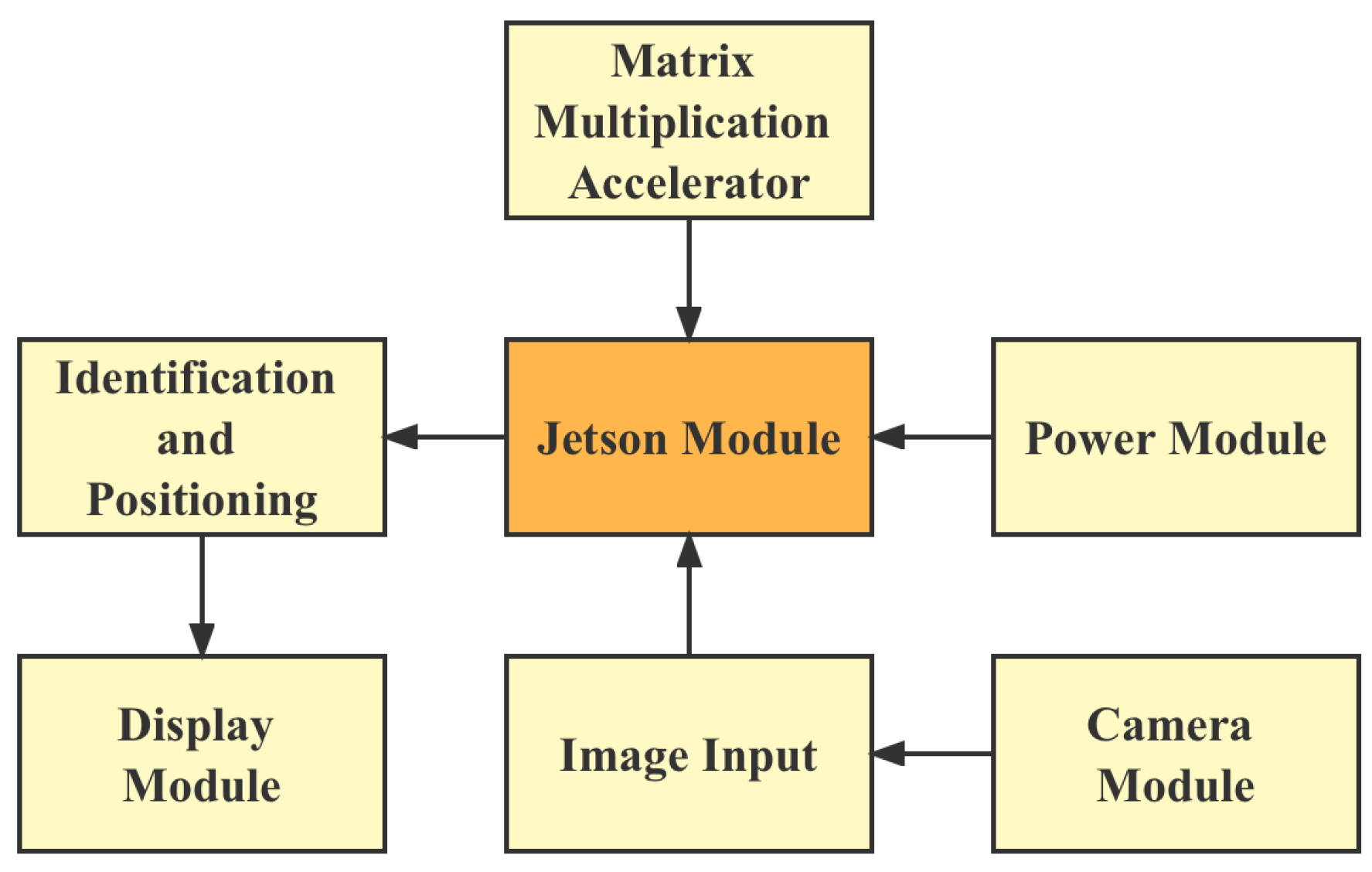
After completing the model training, a plant seedling rapid detection device was designed to realize the rapid detection of plant seedlings, and the hardware system is shown in Figure 12.

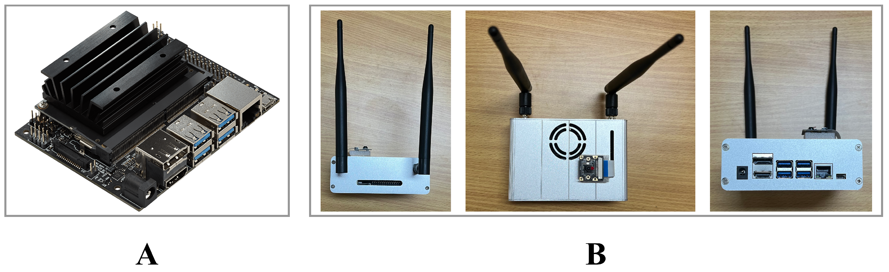
The Jetson logic board is shown in Figure 13A.

A wide-angle camera is installed at the bottom of the device. The logic board is equipped with a USB3.0 interface, an ARM A57 quad-core 1.43 GHz CPU, 4 GB running memory, 16 GB storage, and Ubuntu 20.14 operating system. The results are displayed on an external 3.5″ display, and the video is transmitted via the SPI protocol. It is powered by a Li-ion battery with 5 V-3 A output capability and a 4400 mAh capacity for 9 h of continuous operation of the mobile detection device.

We protected the entire computational body with aluminum, as shown in Figure 13B. The weight of this device is less than 700 g, which is less than the weight of a normal DSLR camera, such as the Canon 5D. This allows the device to be easily mounted on a drone.

8. Conclusions

Seedling detection is an important task in the seedling stage of crops in fine agriculture. The use of drones for fine agriculture to obtain agricultural datasets is becoming increasingly popular. Therefore, this paper aimed at the rapid identification of plant seedlings, collected images of plant seedlings, created an image dataset, and used a deep learning lightweight network training model to develop a deep-learning-based plant seedling rapid detection device. The main innovations are as follows:

• We modified a one-stage object detection network by using deep separable convolution, which significantly reduced the number of model parameters, lowered the model complexity, and improved the model operation efficiency, while maintaining model performance.
• We proposed a multi-activation layer instead of the existing activation function layer to improve the model’s ability to fit complex functions.
• For the situation in which the plant seedlings are not easy to identify in a complex environment, we used a large number of data enhancement methods, and the F1 and mAP of our model can reach 0.95 and 0.89, even if the seedlings are in different lighting conditions.
• Based on the Jetson hardware platform, we developed a portable device and transplanted the network model in this paper for application. The F1 score of the tested video was over 0.87, and the FPS speed was 87.3.

In summary, this paper proposed a high-precision emergence detection scheme based on a UAV platform and developed the corresponding hardware platform.