Validation of a Coupled Simulation for Machine Tool Dynamics Using a Linear Drive Actuator

Abstract

In order to ensure high productivity capabilities of machine tools at a low cost but at increased geometric accuracy, modeling of their static and dynamic behavior is a crucial task in structure optimization. The drive control and the frictional forces acting in feed axes significantly determine the machine’s response in the frequency domain. The aim of this study was the accurate modeling and the experimental investigation of dynamic damping effects using a machine tool test rig with three-axis kinematics. For this purpose, an order-reduced finite element model of the mechanical structure was coupled with models of the drive control and of the non-linear friction behavior. In order to validate the individual models, a new actuator system based on a tubular linear drive was used for frequency response measurements during uniaxial carriage movements. A comparison of the dynamic measurements with the simulation results revealed a good match of amplitudes in the frequency domain by considering dynamic damping. Accordingly, the overall dynamic behavior of machine tool structures can be predicted and thus optimized by a coupled simulation at higher level of detail and by considering the damping effects of friction. Dynamic testing with the newly designed actuator is a prerequisite for model validation and control drive parameterization.

1. Introduction

During the design process, various demands are placed on machine tool structures. Requirements such as high productive capabilities and low manufacturing costs of products, on the one hand, are of an economic nature and aim at the efficient use of a machine tool. On the other hand, there is the demand for high working accuracy to produce high-quality products. These aspects lead to the central objective to enable fast and accurate positioning of tools and workpieces during operation. Linear feed drives are, therefore, central elements determining the dynamic behavior of machine tools [1].

Altintas et al. [2] reviewed the general architecture of feed drive hardware and its computer control structure. The main components of a drive train of modern feed drives are the Computer Numerical Control (CNC) unit, the drive control, the motor, the mechanical system and sensors. The CNC system basically defines the relative movement between a tool and a workpiece. The position and velocity commands, combined with the maximum values of jerk and acceleration, are transmitted to each drive control as the setpoint values of position. If feedforward control is active, velocity or acceleration values are also considered. The task of the servo control and the motor is to move a carriage along the desired path specification with as few deviations as possible despite disturbing influences from the static and dynamic load resulting from the machining operation. Depending on the requirements, either mechanical transmission elements are used to transform the rotary drive motion into a translatory movement or a linear motor drives the carriage directly. The most frequently used transmission elements in machine tools are the ball screw and the rack and pinion drive. In summary, machine tool feed drives are mechatronic systems in which strong interactions between the structure, the drives and the control system occur during positioning or during machining [3].

A detailed investigation of feed drives regarding the impact on the overall machine tool dynamics requires expensive prototyping and intensive testing. Altintas et al. [4] illustrated that virtual prototypes reduce development time and costs and increase quality. They also stated that virtual prototypes can realistically represent the kinematics, their statics and dynamics. Simulation models are examined and tested like real machines. Furthermore, simulation models of feed drives in which the mechanical structure is coupled with the controller system, so-called mechatronic models, are the state of the art [3]; however, they have not yet become popular in the machine tool industry [5].

To model the control subsystem, almost exclusively graphic block-based simulation software is used [6]. This sub-model is coupled with a structural multibody or finite element model with which a synchronized data exchange takes place at each time step [7,8]. Normally, the finite element model for mechatronic system simulation is, on the one hand reduced, in order, and on the other hand, the structural behavior is linearized by one operation position. The latter is not relevant for flexible multibody simulation models, which also allow large carriage movements with small relative displacements of the structure [9,10]. To enable an efficient simulation of the overall mechatronic system, the system matrices of the structural model are usually reduced in order. For the approximation of the dynamic behavior of machine tools, methods based on modal reduction, component mode synthesis (CMS) and modal superposition of the overall model are mainly used [11,12]. Law et al. [13] used the CMS method to predict the position-dependent frequency response function (FRF) at the tool center point of a machine tool. An automatic algorithm was used to include only the most important modes of the substructures to simulate the overall system. To increase the accuracy of the simulation model, Garitaonandia et al. [14] extended the coupling elements between the structural components with local stiffness properties, and Semm et al. [15] included additional local linear damping properties. The influence of control on the dynamic behavior was neglected in all these simulation models. Sato et al. [16] analyzed the influence of drive control with a rigid multibody model in the time and frequency domains. Especially for feed axes with a ball screw drive, the mechanical model must represent the elastic and kinematic conditions in the transmission system. Zaeh et al. [8] described a modeling method for this purpose, transformed the finite element model of a test station for feed drives by means of modal transformation into a state space model and coupled the mechanical model with a control model.

Regardless of the modeling method, a simulation model is supposed to represent reality as closely as possible. With respect to machine tool structures, the mass and stiffness properties of the structural components are known from the design process. The stiffness properties of standardized machine elements such as linear guides, bearings, couplings, ball screws or levelers are specified in their data sheets. However, these data sheets do not contain information about local damping parameters. Brecher et al. [17] presented the identification of local damping values of individual machine elements using special test benches. As far as damping is concerned, the feed drive components show linear behavior in the locked directions, whereas nonlinear friction effects occur in the translational or rotational directions of motion [18]. Rebelein et al. [19] investigated the friction conditions in the spindle bearings, the ball screw drives and the profile rail systems of a test machining center. Based on experimental measurements, friction models of the components were implemented in a reduced flexible multibody simulation model, and the effect of friction on the FRF was depicted. Subsequent publications additionally illustrated the effects of the control parameters and the influence of carriage movements on the damping in the frequency domain [18,20,21].

The already mentioned frequency response function is established for the identification of a machine tool’s behavior. On the one hand, the general dynamic behavior of a machine structure can be evaluated and improved, and on the other hand, the FRFs at the tool center point form the basis of stability studies for machining [22]. Frequency response functions are mostly measured with an impulse hammer; however, depending on the requirements, alternative measuring systems are also used [23,24,25].

This paper presents a modeling approach for predicting the dynamic behavior of machine tools with ball screw drives. The present study focused on the influence of drive control and frictional forces acting in feed axes on frequency response functions. A finite element model of the machine structure was coupled with friction force models and with a model of the drive control. The latter is not limited to a basic structure but contains additional functional modules and filters and also maps the sampling rates of the measuring systems and the computing rates of the digital controller modules. The nonlinear friction models were parameterized with measurements of the drive current during sinusoidal axis movements. This increases the accuracy of the simulation model and enables the investigation of the dynamic behavior during positioning. In order to be able to measure this experimentally as well, a newly developed shaker system for the excitation of the machine structure during uniaxial carriage movements is presented.

2. Methods

In this work, the considered machine structure is a three-axis test machining center with a horizontal main spindle (HSK80) arrangement from the company Fill GmbH, as presented in Figure 1. The kinematics consist of the three translational axes (ball screws) driven by a SIEMENS 840D CNC system. The operating ranges of the individual axes are: X, 1770 mm; Y, 655 mm; and Z, 685 mm.

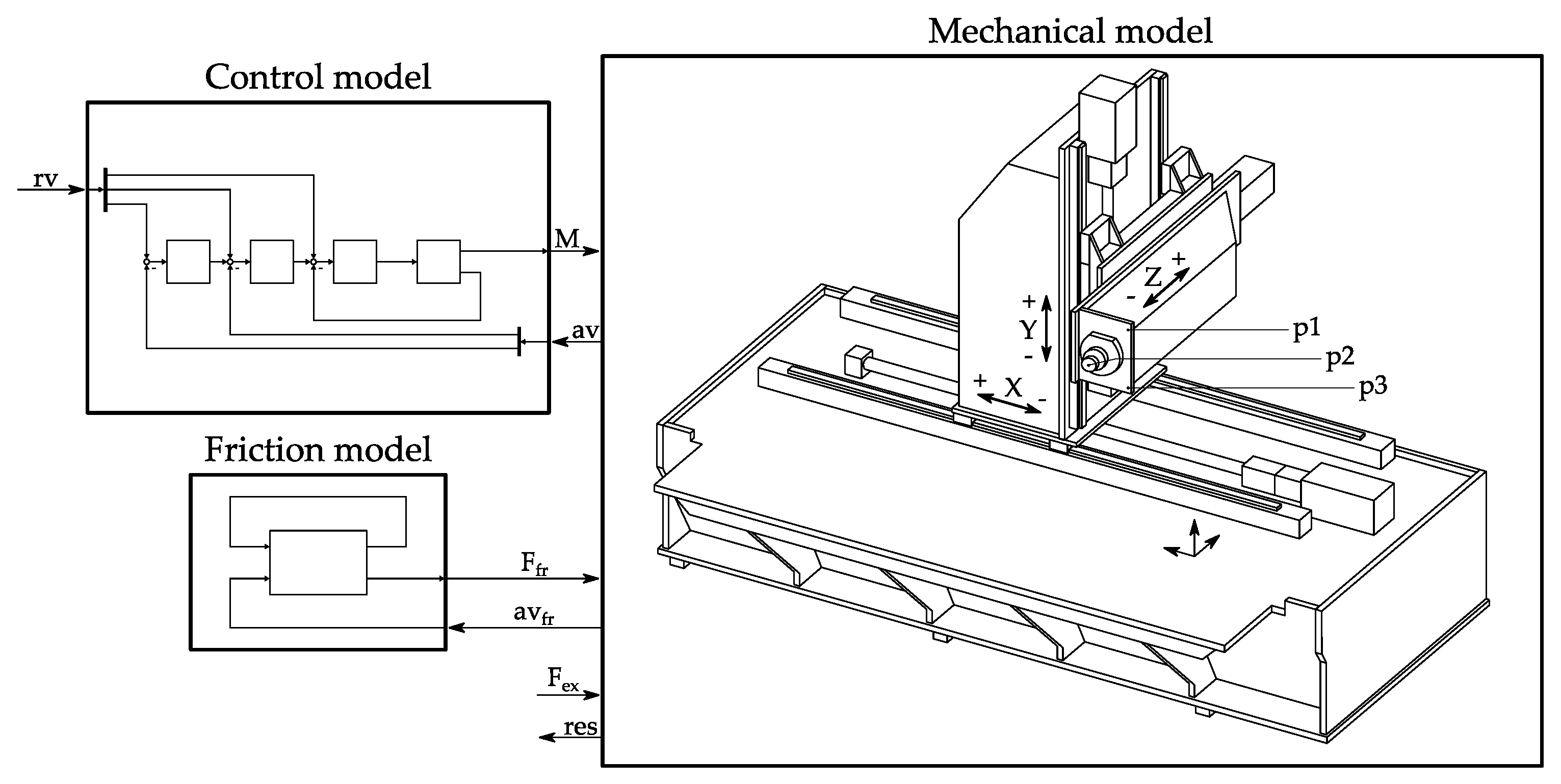
Figure 1 depicts the basic structure of the simulation model for the mechatronic system elaborated in this study. For each individual feed axis, the reference variables (rv) are processed into a drive torque (M) by the modeled controller structure and by an electrical model of the feed drive. The torque is considered as an input into the mechanical model and causes displacements in the modeled direct measuring system as well as velocity changes at the modeled motor encoder. These virtual measured actual values (av) are fed back to the controller model, which eventually results in a closed control system. In order to investigate the influence of friction on the system behavior, a nonlinear friction model is integrated. Using the relative velocity (av_fr) between moving structures and an internal state equation, the resulting friction force (F_fr) is calculated, which, in turn, is considered in the mechanical model. Especially for virtual measurements, external excitation forces (F_ex) can be introduced at any point of the structure, and response signals (res) can also be measured.

With flexible multibody systems, the most comprehensive formulation of the equation of motion including large nonlinear feed drive movements and elastic deformations can be achieved. This advantage is offset by a high modeling effort and the fact that the analysis methods are usually limited to the time domain. However, if rigid body modes are considered in a finite element system, it is also possible, with this method, to capture small movements of subsystems limited to one axis configuration [26]. References [13,14,15] proposed a substructuring approach based on the Craig–Bampton reduction [27] for an efficient simulation at different machine positions and for local design changes. In order to reduce the necessary expert knowledge during modeling and, thus, facilitate the use in an industrial environment, a finite element model of the entire machine is used in this work to define the kinematic, static and dynamic properties of the machine tool structure.

2.1. Finite Element Model

The basic mechanical construction features the tasks of transmitting force or torque flows and generating certain movements. This real, continuous structure is approximated by a finite number of degrees of freedom (DOFs) using the finite element method and can be written in matrix form as a system of n-coupled, linear, second-order, ordinary differential equations (ODEs):

$$\mathit{M}\ddot{\mathit{x}}\left(t\right)+\mathit{C}\dot{\mathit{x}}\left(t\right)+\mathit{K}\mathit{x}\left(t\right)=\mathit{f}\left(t\right)$$

(1)

where $\mathit{x}\left(t\right)$ is the vector of degrees of freedom, $\mathit{M}$ is the mass matrix, $\mathit{C}$ is the viscous damping matrix, $\mathit{K}$ the stiffness matrix and $\mathit{f}\left(t\right)$ is the time-dependent forcing vector [28]. The coefficient matrices completely determine the dynamic structural behavior of the machine and, thus, have to be represented in the model. It should be noted that in the present work, the definition of the damping matrix with local parameters is avoided, and alternatively, the modal damping approach is used.

The structural bodies of the machining center are connected to each other or to the environment by guidance systems, drives or levelers. The machine bed and the individual carriages are steel components and are meshed with volume elements at appropriate geometry, stiffness and mass properties. Modeling of the linear guides with finite elements is inappropriate. Instead, the structural components are connected with linear springs in the vertical and lateral directions. 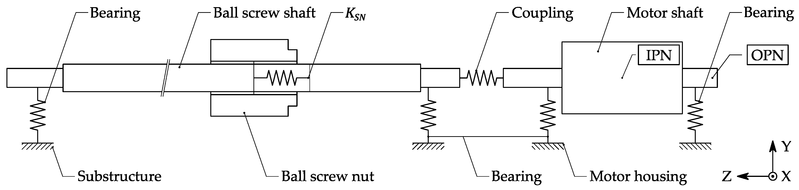Figure 2 presents the general structure of the mechanical drive train of a single axis in the finite element model.

The motor shaft and the ball screw shaft are modeled with three-dimensional elements and are connected to the motor housing and the substructure, respectively, with discrete spring elements. The threads of the ball screw are neglected in the geometric model according to Okwudire et al. [29], and the resulting change in inertia is compensated. However, Schwarz [30] proposed modeling the ball screw shaft with an equivalent instead of the core diameter. The shafts are connected with a torsional stiffness, and the rotary inertia of the coupling is divided equally between the drive and the load side. To model the interface between screw and nut, the approaches of Oertli [6] and Berkermer [26] were combined. This results in the stiffness matrix:

$${\mathit{K}}_{SN}=\left[\begin{array}{cccccc}{k}_X& 0& 0& 0& 0& 0\\ & k_Y& 0& 0& 0& 0\\ & & k_Z& 0& 0& -h_p{k}_Z\\ & & & k_{\psi }& 0& 0\\ & sym& & & k_{\theta }& 0\\ & & & & & h_p^2{k}_Z\end{array}\right],$$

(2)

where $k_{X,Y}$ represents the radial stiffness, $k_Z$ is the axial stiffness, $k_{\psi ,\theta }$ is the tilting stiffness and $h_p$ is a transmission coefficient. All stiffness parameters used in the finite element model were taken directly from the manufacturer’s data sheet or were calculated using geometric relationships.

In order to couple the machine structure with additional models and to enable an efficient simulation of the overall behavior, the mechanical model is represented by a state space model, and the model order is reduced. The following explanations are based on [28]. Assuming a harmonic excitation and neglecting the damping, the generalized eigenvalue problem

$$\left(\mathit{K}-{\omega }^2\mathit{M}\right)\mathit{v}=0$$

(3)

can be derived from the homogenous part of (1). The solutions of (3) are the natural frequencies ${\omega }_i$ and the corresponding mode shapes ${\mathit{v}}_i$, respectively, of the modal matrix

$$\mathit{V}=\left[{\mathit{v}}_1 {\mathit{v}}_2\dots {\mathit{v}}_n\right].$$

(4)

For distinct eigenvalues ${\omega }_i\ne {\omega }_j$, the corresponding modes ${\mathit{v}}_i$ and ${\mathit{v}}_j$ are orthogonal with respect to $\mathit{M}$ as well as to $\mathit{K}$. Due to the orthogonality of the mode shapes, the system matrices are diagonalized and decoupled by post- and pre-multiplying with the modal matrix and its transpose. If the modes are additionally mass normalized and modal damping ${\zeta }_i$ is assumed,

$${\mathit{V}}^T\mathit{M}\mathit{V}=\left[\begin{array}{ccc}1& \cdots & 0\\ ⋮& \ddots & ⋮\\ 0& \cdots & 1\end{array}\right],{\mathit{V}}^T\mathit{C}\mathit{V}=\left[\begin{array}{ccc}2{\zeta }_1{\omega }_1& \cdots & 0\\ ⋮& \ddots & ⋮\\ 0& \cdots & 2{\zeta }_n{\omega }_n\end{array}\right]\mathrm{and}{\mathit{V}}^T\mathit{K}\mathit{V}=\left[\begin{array}{ccc}{\omega }_1^2& \cdots & 0\\ ⋮& \ddots & ⋮\\ 0& \cdots & {\omega }_n^2\end{array}\right]$$

(5)

results. With the modal coordinates $q_i$, the original DOF vector $\mathit{x}$ from (1) can be described with a weighted sum of mode shapes ${\mathit{v}}_i$ by:

$$\mathit{x}={\displaystyle \sum }_{i=1}^n{\mathit{v}}_i{q}_i=\left[{\mathit{v}}_1\dots {\mathit{v}}_n\right]\left[\begin{array}{c}{q}_1\\ ⋮\\ q_n\end{array}\right]=\mathit{V}\mathit{q}.$$

(6)

By inserting (6) into (1) and an additional left multiplication with ${\mathit{V}}^T$,

$${\mathit{V}}^T\mathit{M}\mathit{V}\ddot{\mathit{q}}+{\mathit{V}}^T\mathit{C}\mathit{V}\dot{\mathit{q}}+{\mathit{V}}^T\mathit{K}\mathit{V}\mathit{q}={\mathit{V}}^T\mathit{f},$$

(7)

can be derived with (5) in the equation of motion in modal coordinates for n-un-coupled single DOF oscillators of the form

$${\ddot{q}}_i+2{\zeta }_i{\omega }_i{\dot{q}}_i+{\omega }_i^2{q}_i={\underset{\_}{f}}_i\mathrm{with}\underset{\_}{\mathit{f}}={\mathit{V}}^T\mathit{f}.$$

(8)

If all n modes are considered in (4), the full finite element model is represented in the modal model. The modal order reduction uses the property that with a subset m < n modes, the physical DOFs in (6) can be approximated very well, and thus, the calculation time is reduced.

To reproduce the structural-mechanical behavior in the digital block simulation, the m second-order modal Equation (8) is transformed into a first-order differential equation system. Due to the coordinate transformation

$$\mathit{z}=\left[\begin{array}{c}\mathit{q}\\ \dot{\mathit{q}}\end{array}\right]$$

(9)

Equation (8) becomes

$$\dot{\mathit{z}}=\mathit{A}\mathit{z}+\mathit{B}\mathit{u}$$

(10)

where

$$\mathit{A}=\left[\begin{array}{cc}0& \mathit{I}\\ {\Gamma }_1& {\Gamma }_2\end{array}\right]\mathrm{is}\mathrm{defined}\mathrm{with}{\Gamma }_1=\left[\begin{array}{ccc}-{\omega }_1^2& \cdots & 0\\ ⋮& \ddots & ⋮\\ 0& \cdots & -{\omega }_m^2\end{array}\right]\mathrm{and}{\Gamma }_2=\left[\begin{array}{ccc}-2{\zeta }_1{\omega }_1& \cdots & 0\\ ⋮& \ddots & ⋮\\ 0& \cdots & -2{\zeta }_m{\omega }_m\end{array}\right].$$

(11)

The input matrix

$$\mathit{B}=\left[\begin{array}{c}0\\ {\Gamma }_3\end{array}\right]\mathrm{with}{\Gamma }_3={\mathit{V}}^T{\mathit{F}}_u$$

(12)

contains the unit force matrix ${\mathit{F}}_u$, which is one for degrees of freedom where a force is applied and zero elsewhere. For ball screw drives, this is the torque at the motor rotor and the counter-torque at the motor housing. The former is schematically labeled IPN (input node) in Figure 2. In Equation (10), $\mathit{u}$ represents the vector of the system inputs. The system outputs $\mathit{y}$ (position, velocity and acceleration) are determined via the differential equation system

$$\left[\begin{array}{c}\mathit{y}\\ \dot{\mathit{y}}\\ \ddot{\mathit{y}}\end{array}\right]=\mathit{C}\mathit{z}+\mathit{D}\mathit{u}$$

(13)

where

$$\mathit{C}=\left[\begin{array}{cc}{\Gamma }_4& 0\\ 0& {\Gamma }_4\\ {\Gamma }_4{\Gamma }_1& {\Gamma }_4{\Gamma }_2\end{array}\right]\mathrm{with}{\Gamma }_4={\mathit{U}}_u\mathit{V}.$$

(14)

${\mathit{U}}_u$ is a unit displacement matrix, which is one for degrees of freedom where an output is required and zero elsewhere. With regard to the mechatronic simulation model, these are especially nodes where measuring systems are applied in reality. Figure 2 shows an output node (OPN) of the virtual motor encoder as an example. $\mathit{D}$ in Equation (13) is the feedthrough matrix and is defined as:

$$\mathit{D}=\left[\begin{array}{c}0\\ 0\\ {\Gamma }_4{\Gamma }_3\end{array}\right].$$

(15)

In summary, an undamped modal analysis is used to determine the eigenvalues and eigenvectors of the modeled machine tool structure. By selecting a certain number of modes, the system is model order reduced, with each mode being damped with a proportional damping value. Input and output nodes defined in the model determine where forces are applied in the system or state variables are output, respectively.

2.2. Control Model

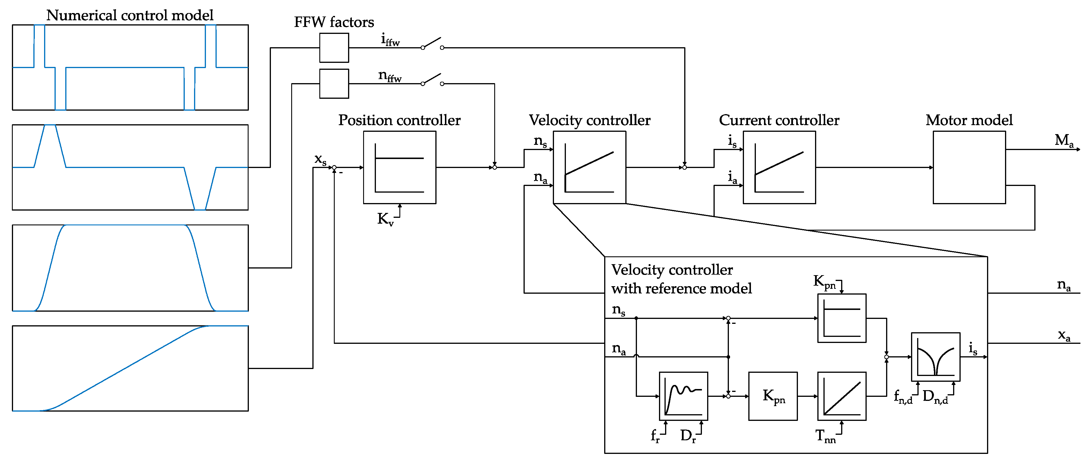
The majority of systems used today for position control of the feed drives of machine tools use a cascaded control loop structure [4]. Figure 3 depicts the basic structure of the control loop of a single axis in the simulation model.

The innermost control loop is formed by the current control, which, together with the motor, is responsible for converting the current setpoint into an actual torque value M_a. The parameters of the current PI controller can be parameterized independently of the machine properties since only electrical values of the drive are fed back into the current control loop. Therefore, the parameters specified by the drive manufacturer are generally suitable [31]. The motor is modeled as a field-oriented controlled synchronous motor. The velocity controller, which compares the setpoint velocity n_s with the measured actual velocity n_a from the motor encoder and generates a torque-proportional setpoint current specification, is also basically designed as a PI controller [4]. The dynamics are determined by the proportional coefficient K_pn, while the integral component with the parameter T_nn ensures that permanent control differences are corrected over time. Modern control systems for machine tools offer the possibility to extend the basic structure with additional function systems and, thus, to influence the dynamic behavior. In the modeled system, it is possible to separate the command and disturbance response of the velocity controller, which is called velocity controller with reference model [32] and is shown in Figure 3. The reference model is a replication of the proportional controlled velocity control loop as a second-order lag element with the undamped natural frequency f_r and the damping value D_r. Furthermore, the reference model delays the setpoint/actual value deviation for the integral component of the velocity controller so that transients can be suppressed when the controller dynamics are high. To attenuate resonances occurring in the mechanical system, current setpoint filters are used in the real control. These are also modeled as general second-order filters and are parameterized by the numerator and denominator natural frequency (f_n and f_d) as well as by the numerator and denominator damping (D_n and D_z), whereas the filter frequencies are mostly in the higher frequency range. The model is designed as a time discrete model, whereby dead times for data transmission and for digital measurement acquisition as well as the computing times of the digital controllers are taken into account. The position controller difference calculated from the actual position value x_a and the position setpoint x_s is converted in the position controller by the proportional value K_v to the reference input for the downstream velocity controller. The position setpoints are calculated with the maximum values of jerk and acceleration and with the user inputs of velocity and position in a numerical control model. Each control loop causes a delay time for the superimposed system, which results in the outer control loops losing dynamics and slower adjustment of reference variable changes [32]. This effect can be compensated by a feedforward control of the inner control loops, whereby a distinction is made between speed and torque feedforward control. If feedforward control is active, the feedforward values calculated in the numerical control model are scaled and delayed with various factors and are subsequently added at the corresponding controllers as reference variables (n_ffw or i_ffw).

2.3. Friction Model

The machining and frictional loads act as external forces on the feed drives of machine tools [2]. Frictional forces as disturbance inputs, which mainly occur during velocity reversal, have to be incorporated and compensated by the control and the drive. However, friction in feed drive components introduces damping into the machine tool system.

Friction force models are used to represent the physical conditions between stationary or moving components. A basic distinction is made between models based on the Coulomb approach and models using the bristle analogy. The former is also called static friction models and show certain weaknesses, especially due to the discontinuity at zero velocity. In dynamic models, the so-called pre-sliding regime is modeled with a function of the relative displacement, whereas in the sliding regime, the friction is a function of the relative velocity [33,34].

In order to investigate friction-specific effects with the mechatronic simulation model, a friction model based on the LuGre model [35] was used. The surfaces between two bodies in contact are visualized by means of elastic bristles. A relative movement of the bodies leads to an elastic deformation of the individual bristles, whereby the sum of the restoring forces caused by the deflections is interpreted as frictional force. As the force increases due to the relative movement, bristles reach their maximum deformation and slip through. The approach based on many bristles is approximated in the model with a single average bristle.

The deflection of the bristle is denoted by z and is used to represent the frictional dynamics in the pre-sliding regime. The frictional force is defined as:

$$F={\sigma }_{0}z+{\sigma }_1\frac{dz}{dt}+{\sigma }_{2}v,$$

(16)

where ${\sigma }_0$ describes the stiffness of the bristle, ${\sigma }_1$ is the micro viscous damping factor, ${\sigma }_2$ is the viscous damping factor and $v$ is the relative velocity between the two surfaces.

The internal state is modeled with the nonlinear differential equation

$$\frac{dz}{dt}=v-\frac{\left|v\right|}{g\left(v\right)}z.$$

(17)

The friction force $F$ converges in the sliding regime against the stationary friction behavior represented by the function $g\left(v\right)$ and the viscous component. The function $g\left(v\right)$ can contain any functional dependencies and can be parameterized by measuring the friction force at constant velocities. According to [36], $g\left(v\right)$ is modeled as:

$$g\left(v\right)=\left(F_C+\left(F_S-F_C\right)e^{-{\left(\frac{\left|v\right|}{v_S}\right)}^{\beta }}+F_{log}\ln \left(\frac{\left|v\right|}{v_{log}}+1\right)\right)\frac{1}{{\sigma }_0},$$

(18)

where $F_C$ represents the Coulomb friction, $F_S$ is the static friction, $v_S$ is the Stribeck velocity, $\beta$ constitutes the shape factor and $F_{log}$ and $v_{log}$ represent the logarithmic friction components.

The friction parameters of individual, unloaded feed drive components can be metrologically identified either with a sequential assembly process approach or with the test bench approach [19]. In the present contribution, the total frictional force of the feed axes in real operation was determined through the respective motor current, and a single friction model for each axis was deposited in the simulation—a so-called machine approach. Thus, the load and assembly conditions of the entire machine are taken into account, and the friction models are adapted for real operations. 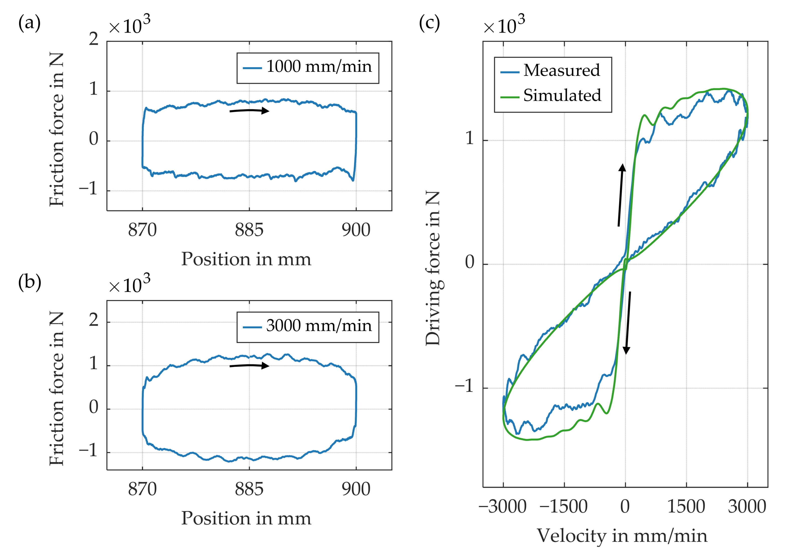Figure 4a,b present the determined friction curves for a sinusoidal movement of the X-axis (see Figure 1). The drive current was measured with an internal measuring function of the CNC system and then converted into a drive force using the torque constant and the spindle pitch. The time-dependent acceleration forces were subtracted from the driving forces, and the resulting friction forces are shown as a function of position.

The transitions between pre-sliding and sliding regime differ, on the one hand, from the feed rate and, on the other hand, from the acceleration direction. Based on these measurements, the lumped friction models of the individual feed drives were parameterized. Figure 4c depicts the comparison between the measured and simulated total driving forces of the X-axis.

2.4. Experimental Setup

The dynamic properties of a machine tool significantly determine the productivity of the system and the quality of the manufactured components. The frequency response function (FRF) as a relationship between the input (force) and the output (acceleration, velocity or position) of a system describes these characteristics in the frequency domain and can be measured. Generally, two different excitation techniques are used for this purpose: impact and shaker excitation [37]. The former is a very convenient, fast and popular measuring method where, on discrete points of a structure, the impact force and the response are measured. In contrast to tap testing, the measurement setup for shaker excitation is more complex. However, for shaker testing, many types of excitation signals are available, and in general, it is more repeatable. As far as the different types of shakers are concerned, electrodynamic, electrohydraulic and piezoelectric exciters are the most common for the investigation of machine dynamics [24]. In particular, these systems differ with regard to the maximum excitation frequency, the maximum excitation force and the suitability for absolute or relative excitation. With the already mentioned shaker types, however, a relative excitation during feed drive positioning is not possible. Therefore, a shaker system for frequency response measurements in machine tools during uniaxial linear carriage movements was developed; see Figure 5.

The excitation force is generated by a conventional, electromagnetic linear motor in tubular form; see Figure 5a. Thus, forces up to 500 N can be introduced into the system in the frequency range up to about 250 Hz. Due to the severe attenuation of the force after exceeding the first mechanical natural frequency of the shaker system and due to the electrodynamic limits, the force which is available for the excitation of the test object decreases in the higher frequency range [36]. This must be taken into account for measurements up to 1000 Hz, whereas in this research, only the lower frequency range is of interest. The excitation force is measured with a piezoelectric force transducer which is connected to the linear motor slider by a stinger (see Figure 5a). The motor is controlled by a voltage signal proportional to the current or force. An additional position encoder is built into the system to measure the current displacement. The power supply and the data acquisition device (DAQ) are implemented in a portable case, as depicted in Figure 5b. The structural response is measured by means of accelerometers, and the motor control and measurement signal evaluation is performed in a single software environment. Figure 5c shows the experimental setup for the dynamic investigation of the machining center from Figure 1. With this type of machine, the workpiece is usually positioned in the machining area with the help of a rotary table. In the test execution, the rotary table was omitted, so the workpiece clamping was replaced by a steel block. On the tool side, the shaker was connected directly to the tool interface.

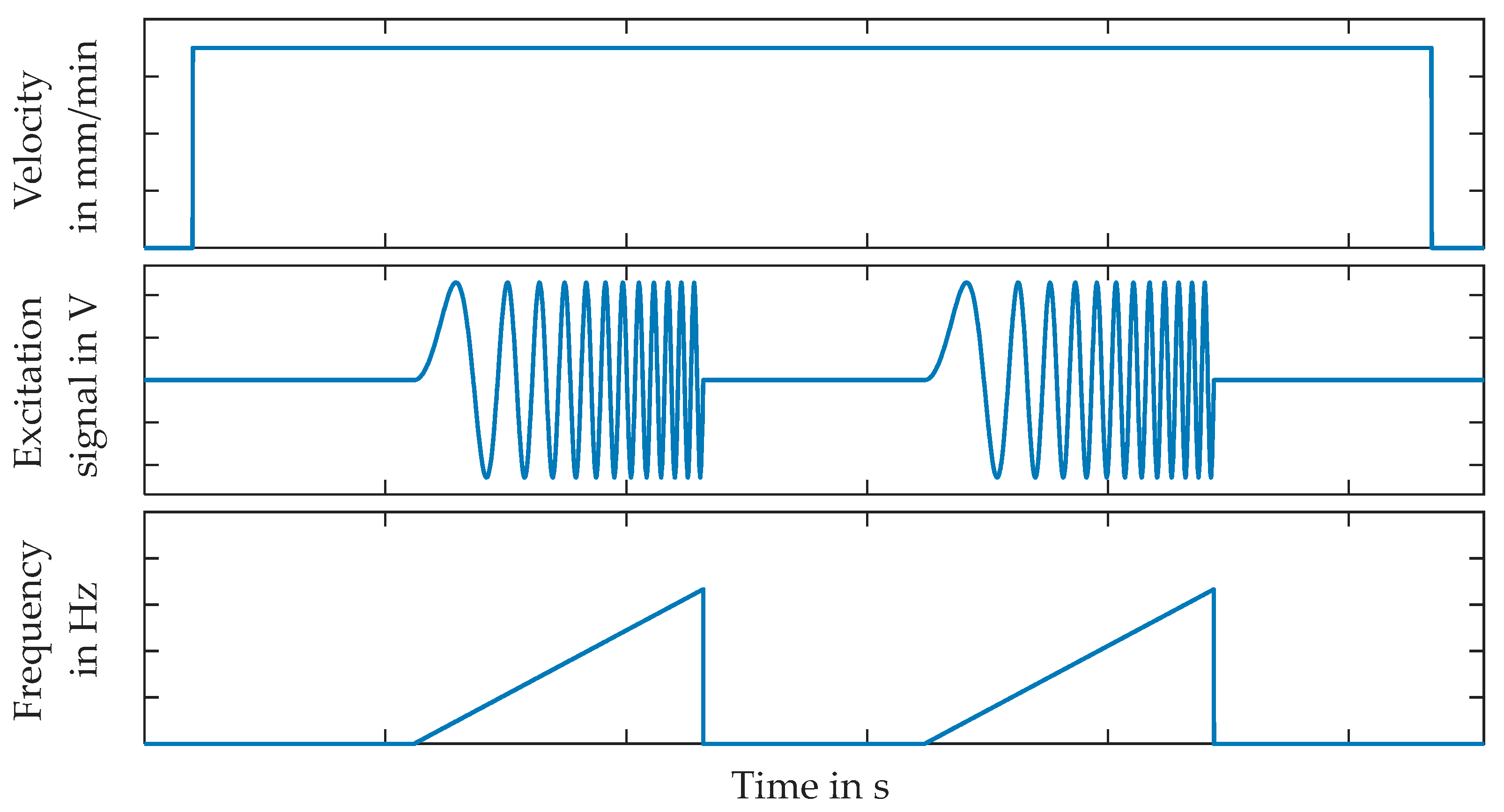
The long-stroke shaker is fed with a sine chirp modulation signal, whereby basically any signal type can be applied for modal analysis. In order to measure the dynamic behavior during positioning, the feed drive is accelerated to a constant velocity, and subsequently, the motor is fed with the excitation signal, as shown in Figure 6.

However, the feed rate is limited by the signal length, by the number of iterations and by the maximum motor stroke of 70 mm. The mean values of the measured input signal (force) and of the measured response signals (acceleration) are removed; afterwards, the auto-power and cross-power spectra are averaged over the number of iterations, and finally, the frequency response function is calculated.

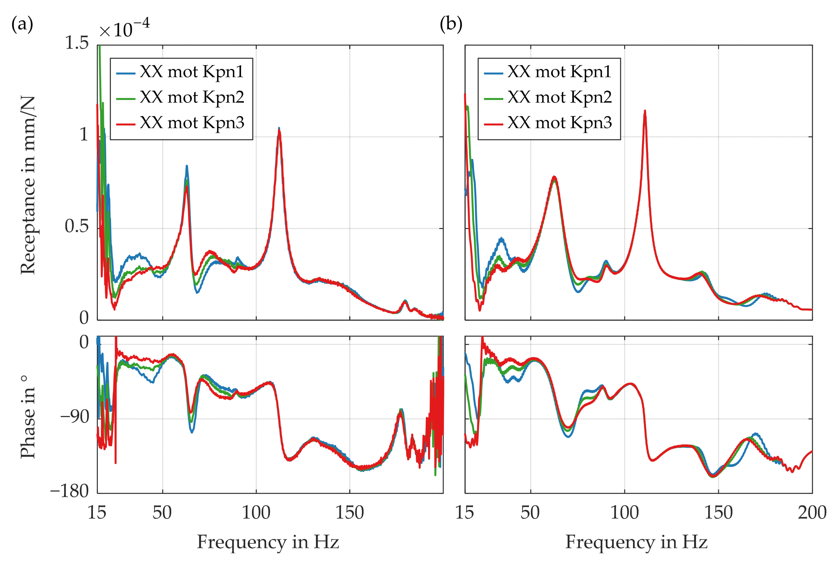
For validation, the dynamic properties of the machining center were determined at different axis positions with an impulse hammer and, subsequently, with the presented long-stroke shaker. The axis positions and the FRF investigation properties of the executed measurements and simulations are summarized in

Table 1. Excitation characteristics and measuring and axis positions during measurements/simulations.

	S1	S2
Excitation	Absolute	Relative
Excitation signal type	Impulse	Sine chirp
Excitation point	p1	p2
Excitation direction	X/Y/Z	X
Excitation force in N	-	250
L/U frequency in Hz	-	1/200
Measuring point	p3	p3
Position X-axis in mm	885	855
Position Y-axis in mm	327	373
Position Z-axis in mm	0	342

.

Additionally, the system was tested under three different boundary conditions: with active motor brake at rest (br), with active feed drive control (ctrl) and during uniaxial carriage movements (mot). The mechanical structural modes up to 200 Hz were of interest, and the measurement parameters were chosen accordingly. Figure 1 shows the points p1, p2 and p3 where the structure was excited and the response was measured.

3. Results and Discussion

An experimental modal analysis of the machine tool structure was carried out to validate the mass and stiffness matrices used in the finite element model. Figure 7 shows the comparison between the measured and simulated axial frequency response functions with modal damping and with active motor brake. The latter was implemented in the simulation model by fixing the motor rotor to the housing.

It is evident that the dominant natural frequencies and mode shapes between 20 and 100 Hz identified from the measurements can be predicted with a very high accuracy by means of simulation. Slight deviations occur in the resonance amplitudes at approximately 55 Hz in the Y-direction and at 75 Hz in the X-direction, whereby the simulated eigenvalues in the frequency range deviate by a maximum of 4 Hz.

During shaker excitation, a closed force flow is generated in the structure and thus simulates the machining forces between the workpiece and tool. For the experimental investigations, the tool was omitted (see Figure 5c) because only structural modes in the lower frequency range were of interest. As already mentioned, the reduced state space model calculated from the finite element model represents the static and dynamic properties of the structure only for the modeled axis position. The FE model is designed in such a way that the virtual machine tool can be repositioned with three parameters. Subsequently, a valid state space model is generated again without further modeling effort. For the comparison in state S2, the feed carriages were thus repositioned in the simulation model and the shaker clamping was integrated. In [20], Rebelein et al. pointed out that out of the drive components, the profiled rail systems constitute the largest proportion of the overall friction. Therefore, output nodes (OPNs) and input nodes (IPNs) on the linear guide rails/shoes were defined in order to be able to measure the relative velocity on the one hand and to introduce friction forces into the system on the other hand. The friction generates a damping force in the axial direction; consequently, the linear modal damping was reduced at those frequencies that show an increased amplitude in the respective direction. The friction models of the individual axis, parameterized by the procedure described in Section 2.3, were coupled with the mechanical structure model. Figure 8 depicts the comparison between an FRF measured with the long-stroke shaker and an FRF resulting from the simulation model with integrated nonlinear friction models. By means of the linear motor, sufficient energy is introduced into the machine tool during relative excitation in order to measure a response with the accelerometers, even in the low frequency range. The frequency response function presented in Figure 8a underlines the performance of the developed measurement system.

By modifying the axis positions, the modes at 74 and 100 Hz (see Figure 7a) shift to higher frequencies (110 and 122 Hz), whereas the remaining natural frequencies are only slightly or not at all influenced. It can be derived from Figure 8b that the simulation model also depicts the position-dependent behavior and, in addition, that the coupled friction models damp the modes accordingly. However, the measured mode at 75 Hz is underrepresented in the finite element model, and the damping at 38 Hz deviates slightly. Due to the nonlinear friction, the simulation model behaves as a function of the magnitude of the excitation force. Therefore, the measured shaker force (sine chirp) was used as input signal, and the frequency response function was calculated with the results of transient simulation.

Figure 9a shows the dynamic behavior of the machining center with the active motor brake in comparison with the machine tool axes in a controlled state and with feed rate at zero. The proportional gains, integral time constants and the other controller parameters were tuned to an optimal state. With active control and excitation in X-direction, the mode at 122 Hz (axial mode of the Z-axis) is completely attenuated. The parameter sets including the settings of calculation times, feedforward control, reference model and filters were imported into the simulation model, and the predicted frequency response function with active control is presented in Figure 9b. Comparing the results of the simulation with those of the experiment, the major trends of the measurement are also revealed in the simulation model with a very high accuracy.

Finally, the machine tool structure was excited with the long-stroke shaker during positioning motion with a constant feed rate of 100 mm/min of the X-axis. Figure 10a depicts the measured receptance with active speed feedforward control and a variation of the velocity proportional gain K_pn of the X-axis velocity controller. The influence of the proportional gain to the frequency response function is quite well predicted by simulation, as shown in Figure 10b. The parameter noticeably affects the eigenvalues as well the damping of the first two modes. Consequently, a high gain value results in a higher amplitude and a lower eigenvalue compared to a parameterization with a low-velocity proportional gain.

4. Conclusions

The accurate prediction of dynamic properties is a crucial task in the development process of machine tools. In the present contribution, models of the mechanical structure, drive control and frictional forces acting in feed axes of a three-axis test machining center were coupled and the simulation behavior was subsequently compared with measurements. A newly developed actuator system based on a tubular linear motor is presented as a means of measuring frequency response functions during uniaxial carriage movements. It revealed that the structural–mechanical properties are very well represented with a state space model reduced from a finite element model. The parameterization of the coupled stiffnesses with values from the manufacturer’s data sheet provides sufficient accuracy for dynamic investigations, and the position dependence is also taken into account with the presented modelling method. Due to the column design and the kinematic structure of the machine under investigation, the interactions between the machine’s structure and the controlled drives significantly influences the measured and also the simulated frequency responses. Measurements of the drive current during sinusoidal carriage movements were used to parameterize nonlinear friction models for the individual axes. These damp the system accordingly; however, there is still potential for improvements regarding the accuracy at constant velocity and the distribution of the friction forces to the individual components. The influence of the velocity proportional gain on the dynamic compliance during positioning was shown by the simulation and confirmed by measurements. To summarize, the dynamic properties of the machining center at the tool center point can be predicted in the frequency range up to 200 Hz with the presented mechatronic simulation model. During development, design changes can thus be analyzed fast and accurately, which consequently leads to an improvement in machine performance. The frequency response functions up to 200 Hz obtained with the presented actuator system show a very high quality and a remarkable repeatability, and the system is thus suitable to analyze the dynamic structural behavior of machine tools. The portable design, the automated measurement process and the possibility of excitation in compliance with machine safety enables industrial use.

The presented modeling approach will be used in the future to study the prediction accuracy in motion trajectories. In addition, the position dependence with respect to the influence of the control parameters and the friction should be systematically determined in further investigations. For this purpose, the long-stroke shaker represents a suitable actuating system, whereby the data recorded by the internal feed drive measuring system may additionally be considered for these analyses. Further experimental tests are necessary to determine the maximum possible excitation frequency of the shaker and, thus, its suitability for higher-frequency investigations.