On the Use of Molecular Dynamics Simulations for Elucidating Fine Structural, Physico-Chemical and Thermomechanical Properties of Lignocellulosic Systems: Historical and Future Perspectives

Abstract

The use of Molecular Dynamics (MD) simulations for predicting subtle structural, thermomechanical and related characteristics of lignocellulosic systems is studied. A historical perspective and the current state of the art are discussed. The use of parameterised MD force fields, scaling up simulations via high performance computing and intrinsic molecular mechanisms influencing the mechanical, thermal and chemical characteristics of lignocellulosic systems and how these can be predicted and modelled using MD is shown. Individual discussions on the MD simulations of the lignin, cellulose, lignin-carbohydrate complex (LCC) and how MD can elucidate the role of water on the surface and microstructural characteristics of these lignocellulosic systems is shown. In addition, the use of MD for unearthing molecular mechanisms behind lignin-enzyme interactions during precipitation processes and the deforming/structure weakening brought about by cellulosic interactions in some lignocellulosic systems is both predicted and quantified. MD results from relatively smaller systems comprised of several hundred to a few thousand atoms and massive multi-million atom systems are both discussed. The versatility and effectiveness of MD based on its ability to provide viable predictions from both smaller and massive starting systems is presented in detail.

1. Introduction

1.1. Molecular Dynamics and Associated Force Fields

Molecular dynamics (MD) simulations, first developed in the late 1970s for protein folding and conformational analyses, have advanced from simulating several hundreds of atoms to systems with several thousand or even millions of atoms [1,2,3]. The methodology of MD involves:

• Simulating the motions of particles (atoms, molecules, granules, etc.) via a classical approach;
• Solving Newton’s second law for the motions of all of the particles [1,2,3].

MD is the most efficient and widely used numerical approach for studying thermodynamic properties in atomic and molecular systems. In MD, atoms with initial positions and velocities are exposed to collisions governed by the empirical interatomic potentials (EIP). As a consequence of these collisions, the atoms making up the simulated system occupy several different coordinate positions based on time. Such a system can, in effect, be defined by a mathematical expression that correlates total energy to particle coordinates. This expression is known as a force field. Generically, a force field can be expressed in analytical form as U (r₁, r₂, r₃, … r_n) where r represents the positional coordinates.

Before carrying out an MD simulation, information is required about the initial positions (r), velocity (v), charge (q) and bond information (type of atoms, bond angles, lengths, etc). To run a simulation, in addition to above, information is also needed about the force acting on each particle and the overall acceleration. These parameters are typically obtained either from ab-initio/semi-empirical quantum mechanical calculations or by fitting to experimental data such as neutron, X-ray and electron diffraction, Nuclear Magnetic Resonance (NMR), infra-red (IR), Raman and neutron spectroscopy. The molecules are simply defined as a set of atoms that are held together by simple elastic (harmonic) forces and the force field replaces the true potential with a simplified model valid in the region being simulated. Ideally, the force field expression must be simple enough to be evaluated quickly, but sufficiently detailed to reproduce the properties of interest of the system being studied.

In an MD simulation, all of the atoms are treated as point masses and all the electrons are assumed to be in the ground state. To determine the positions of the various atoms at different simulation times, methods such as the Verlet algorithm [4] are used to solve the equations of motion. If the initial position of the atom is given by $\mathrm{r}\left(\mathrm{t}\right)$, then the position in the next time step given by $\mathrm{r}\left(\mathrm{t} + \mathsf{\Delta }\mathrm{t}\right)$ can be described in terms of $\mathrm{r}\left(\mathrm{t}\right)$ and the current acceleration $\mathrm{a}\left(\mathrm{t}\right)$ as shown in Equation (1) to Equation (4) where $\mathrm{O}\left({\mathsf{\Delta }\mathrm{t}}^4\right)$ is the 4th order error term of the polynomial expression in Equation (1).

$$\mathrm{r}\left(\mathrm{t} + \mathsf{\Delta }\mathrm{t}\right)=\mathrm{r}\left(\mathrm{t}\right)+\mathrm{v}\left(\mathrm{t}\right)\mathsf{\Delta }\mathrm{t}+\frac{1}{2}\mathrm{a}\left(\mathrm{t}\right){\mathsf{\Delta }\mathrm{t}}^2+\frac{1}{3!}{\mathrm{r}}^{\dots }\left(\mathrm{t}\right){\mathsf{\Delta }\mathrm{t}}^3+\mathrm{O}\left({\mathsf{\Delta }\mathrm{t}}^4\right)$$

(1)

$$\mathrm{r}\left(\mathrm{t}-\mathsf{\Delta }\mathrm{t}\right)=\mathrm{r}\left(\mathrm{t}\right)-\mathrm{v}\left(\mathrm{t}\right)\mathsf{\Delta }\mathrm{t}+\frac{1}{2}\mathrm{a}\left(\mathrm{t}\right){\mathsf{\Delta }\mathrm{t}}^2-\frac{1}{3!}{\mathrm{r}}^{\dots }\left(\mathrm{t}\right){\mathsf{\Delta }\mathrm{t}}^3+\mathrm{O}\left({\mathsf{\Delta }\mathrm{t}}^4\right)$$

(2)

$$\mathrm{r}\left(\mathrm{t}+\mathsf{\Delta }\mathrm{t}\right)+ \mathrm{r}\left(\mathrm{t}-\mathsf{\Delta }\mathrm{t}\right)=2\mathrm{r}\left(\mathrm{t}\right)+ \mathrm{a}\left(\mathrm{t}\right){\mathsf{\Delta }\mathrm{t}}^2+\mathrm{O}\left({\mathsf{\Delta }\mathrm{t}}^4\right)$$

(3)

$$\mathrm{r}\left(\mathrm{t}+\mathsf{\Delta }\mathrm{t}\right)= 2\mathrm{r}\left(\mathrm{t}\right)- \mathrm{r}\left(\mathrm{t}-\mathsf{\Delta }\mathrm{t}\right)+\mathrm{a}\left(\mathrm{t}\right){\mathsf{\Delta }\mathrm{t}}^2+\mathrm{O}\left({\mathsf{\Delta }\mathrm{t}}^4\right)$$

(4)

Next, the individual atoms making up the simulated molecule are described using a potential energy function $\mathrm{U}\left(\mathrm{R}\right)$ given by:

$$\frac{{\mathrm{d}}^2{\mathrm{R}}_{\mathrm{i}}}{{\mathrm{dt}}^2}= -\frac{1}{{\mathrm{m}}_{\mathrm{i}}}{\nabla }_{\mathrm{i}}\mathrm{U}\left(\mathrm{R}\right)$$

(5)

Equation (5) is then solved, subject to the following initial conditions, R = R (0) and vs. = vs. (0) and applying relevant boundary conditions (R_i, v_i, and m_i are position and velocity and mass of atom (i). Defining the inter- and intra-atomic and molecular interactions happening within the simulation box involves solving the electronic Schrödinger equation for each atom in the system. This becomes extremely complicated, especially in a polymeric system with several hundreds or thousands of atoms. Therefore, analytical representations of the potential surface inside the box are utilised. For instance, it is possible to express the overall potential energy of the system (U_pot) as:

$${\mathrm{U}}_{\mathrm{pot}}={ \mathrm{U}}_{\mathrm{bond}}+{ \mathrm{U}}_{\mathrm{non} \mathrm{bond}}$$

(6)

U_bond potentials arise because of near neighbour connections in the molecular structure. U_non-bond potentials depend upon the distance between the interacting species. These non-bonded potentials are calculated between atoms belonging either to the same chain (but separated by more than two or three bonds depending on the definition of the torsional potential) or to different molecules.

Depending on the different ways of defining U_bond and U_non-bond there are several different force fields. A generic example is shown in Equation (7) wherein the first four terms constitute the intramolecular terms U_bond. The last two terms represent the repulsive and van der Waals interactions (by means of a 12,6 Lennard–Jones type potential) and the Coulombic interactions and constitute U_{non- bond}. In Equation (7), r, θ, q and g denote bond length, bond angle, improper and proper dihedral angles while r₀, θ_0, q₀ and g₀ are the equilibrium values, k_d, k_θ, k_ϕ and k_g are the associated force constants with n being the periodicity of the torsional potential. r_ij is the distance between the two non-bonded atoms i and j, ε_ij and σ_ij are the well depth and contact radius of the Lennard–Jones potential between these atoms, c_i and c_j are the charges on i and j, ε₀ is the vacuum permittivity (8.854 × 10⁻¹² C² J⁻¹m⁻¹) and ε is the effective dielectric constant of the medium.

$$\begin{array}{l}{\mathrm{U}}_{\mathrm{pot}}={\displaystyle \sum _{\mathrm{bonds}}}\frac{{\mathrm{k}}_{\mathrm{d}}}{2}{\left(\mathrm{r}-{\mathrm{r}}_0\right)}^2+{\displaystyle \sum _{\mathrm{bond} \mathrm{angles}}}\frac{{\mathrm{k}}_{\mathsf{\theta }}}{2}{\left(\mathsf{\theta }-{\mathsf{\theta }}_0\right)}^2{\displaystyle \sum _{\mathrm{improper} \mathrm{dihedrals}}}\frac{{\mathrm{k}}_{\varnothing }}{2}{\left(\mathrm{q}-{\mathrm{q}}_0\right)}^2 \\ + {\displaystyle \sum _{\mathrm{torsion}}}\frac{{\mathrm{k}}_{\tau }}{2}[1-\cos \left(\mathrm{ng}-{\mathrm{g}}_0\right)] +{\displaystyle \sum _{\mathrm{non}-\mathrm{bonded}}}4{\mathsf{\epsilon }}_{\mathrm{ij}}\left[{\left(\frac{{\mathsf{\sigma }}_{\mathrm{ij}}}{{\mathrm{r}}_{\mathrm{ij}}}\right)}^{12}-{\left(\frac{{\mathsf{\sigma }}_{\mathrm{ij}}}{{\mathrm{r}}_{\mathrm{ij}}}\right)}^6\right]\\ + \frac{1}{4{\mathsf{\pi }\mathsf{\epsilon }\mathsf{\epsilon }}_0}\frac{{\mathrm{c}}_{\mathrm{i}}{\mathrm{c}}_{\mathrm{j}}}{{\mathrm{r}}_{\mathrm{ij}}}\end{array}$$

(7)

One of the major limitations of MD can be seen from the expressions used to define the intramolecular bonds. The first term in Equation (7), represents the dynamics of bond stretching and squeezing and is of a simple harmonic form. The values for r₀ can be obtained using Raman spectroscopy or from X-ray diffraction experiments. However, the use of the harmonic function implies that the bond cannot be broken, so no chemical processes can be studied. This is one of the main limitations of force field-based MD simulations compared to ab-initio MD. The second term in Equation (7) is for angular bending of the bonds and is also represented using a harmonic potential as in Equation (8) but in some cases a trigonometric potential can also be used as shown in Equation (9).

$${\mathrm{U}}_{\mathrm{bend}}={\displaystyle \sum }_{\mathrm{angles}}\frac{{\mathrm{k}}_{\mathrm{b}}}{2}{\left(\mathsf{\theta }-{\mathsf{\theta }}_0\right)}^2$$

(8)

$${\mathrm{U}}_{\mathrm{bend}}={\displaystyle \sum }_{\mathrm{angles}}\frac{{\mathrm{k}}_{\mathrm{b}}}{2}{(\cos \mathsf{\theta }-\cos {\mathsf{\theta }}_0)}^2$$

(9)

As angle bending is also associated with vibrational movements, additional harmonic terms are sometimes added to the U_bend term as shown in Equation (10) where ‘s’ represents the distance between the two atoms forming the bond and is referred to as the Urey–Bradley or U-B potential.

$${\mathrm{U}}_{\mathrm{vib}}={\displaystyle \sum }_{\mathrm{angles}}\frac{{\mathrm{k}}_{\mathrm{b}}}{2}{\left(\mathrm{s}-{\mathrm{s}}_0\right)}^2$$

(10)

The third term in Equation (7) represents the torsion observed in any molecule containing more than four atoms in a row. Torsional motions are less stiff than bond stretching motions and are necessary for ensuring the correct degree of rigidity of the molecule and to reproduce the major conformational changes due to bond rotation. For polymers and other macromolecules, this is an extremely important term as it helps determine the local structure and relative stability thereof. However, an additional term is needed with the torsional terms to ensure planarity for some types of bonding systems such as sp² hybridized carbon atoms in carbonyls or aromatic rings. This extra component describes the positive contribution to the energy of those out-of-plane motions and is shown in Equation (11) where $\mathsf{\lambda }$ is the improper angle corresponding to the deviation from planarity. An alternative to Equation (11) is shown in Equation (12).

$${\mathrm{U}}_{\mathrm{imp}}={\displaystyle \sum }_{\mathrm{impropers}}\frac{{\mathrm{k}}_{\mathrm{imp}}}{2}[1+\cos \left(2\mathsf{\lambda }-\mathsf{\pi }\right)]$$

(11)

$${\mathrm{U}}_{\mathrm{vib}}={\displaystyle \sum }_{\mathrm{impropers}}\frac{{\mathrm{k}}_{\mathrm{imp}}}{2}{\left(\mathsf{\lambda }-{\mathsf{\lambda }}_0\right)}^2$$

(12)

The first of the two intermolecular/ non-bonding terms used in Equation (7) represent the repulsive and attractive van der Waals forces between the atoms. The repulsion is a consequence of the overlap of the electronic orbitals of both atoms while the interaction between the induced dipoles leads to an attractive force. These two forces vary as different power functions of the interatomic distance. Non-bonded interactions are usually excluded between atoms which are already interacting by a bond or bond angle term (first and second neighbours) and they are often modified for the end atoms of a dihedral angle (third neighbours). van der Waals forces act between any pair of atoms belonging to different molecules, but they also intervene between atoms belonging to the same molecule that are sufficiently separated, as described later. It is possible to define a set of parameters (e.g., $\mathsf{\sigma }$_ij and ${\mathsf{\epsilon }}_{\mathrm{ij}}$) for each different pair of atoms, but for convenience most force fields give individual atomic parameters (i.e., ${\mathsf{\sigma }}_{\mathrm{i}}$ and ${\mathsf{\epsilon }}_{\mathrm{i}}$), together with some rules to combine them. The Lennard–Jones parameters for pairs of unlike atoms are often derived by mixing rules, e.g., the Lorentz-Berthelot combining rules shown in Equations (13) and (14) [5]:

$${\mathsf{\epsilon }}_{\mathrm{ij}}= \sqrt{{\mathsf{\epsilon }}_{\mathrm{ii}}{\mathsf{\epsilon }}_{\mathrm{jj}}}$$

(13)

$${\mathsf{\sigma }}_{\mathrm{ij}}= \frac{{\mathsf{\sigma }}_{\mathrm{ii}}+{ \mathsf{\sigma }}_{\mathrm{jj}}}{2}$$

(14)

Depending on the type of forcefields used, the forms of the individual terms may vary. For instance, a different expression may be used for non-bonded van der Waal’s interaction like the Lennard–Jones 9, 6 potential [6] instead of the 12, 6 expression shown in Equation (7). The final term in Equation (7) serves to describe the electrostatic interactions. Some force fields can also include cross terms between different degrees of freedom/ interactions. These are good for describing the coupling between stretching, bending, and torsion. They bring corrections to the intramolecular energy and allow to better reproduce the observed spectra of intramolecular vibrations. Some examples of cross terms are U_bond-bond, U_bond-bend and U_H-Bonding and are shown in Equations (15)–(17) where r_AD is the distance between the donor and the acceptor atoms, and $\mathsf{\theta }$_AHD is the angle between the donor, the hydrogen, and the acceptor atoms.

$${\mathrm{U}}_{\mathrm{bond}-\mathrm{bond}}= \frac{{\mathrm{k}}_{\mathrm{bb}}}{2}\left(\mathrm{r}-{\mathrm{r}}_0\right)\left( {\mathrm{r}}^{\prime }-{\mathrm{r}}_0^{\prime }\right)$$

(15)

$${\mathrm{U}}_{\mathrm{bond}-\mathrm{bend}}= \frac{{\mathrm{k}}_{\mathrm{b} {\mathrm{b}}^{\prime }}}{2}\left[\left(\mathrm{r}-{\mathrm{r}}_0\right)\left( {\mathrm{r}}^{\prime }-{\mathrm{r}}_0^{\prime }\right)\right]$$

(16)

$${\mathrm{U}}_{\mathrm{H}-\mathrm{bonding}}=\left[\left(\frac{\mathrm{A}}{{\mathrm{r}}_{\mathrm{AD}}{}^{12}}\right)-\left(\frac{\mathrm{B}}{{\mathrm{r}}_{\mathrm{AD}}{}^{10}}\right)\right]{\cos }^2{\mathsf{\theta }}_{\mathrm{AHD}}$$

(17)

The final aspect of MD force fields is the mechanism by which polarizability can be introduced into the system. In a condensed matter system, the emergence of local electric fields induces the appearance of dipoles in the system and describing only the average polarization through the entire system is not enough as local effects are not described well enough by the average value. Essentially, the simulated molecule would behave the same way irrespective of the state it is in or the medium it has been dispersed in. Interactions such as solvation, H- bond directionality and cation-aromatic interactions cannot be effectively modelled. Hence, most modern forcefields explicitly include the polarization. In this case, for each atom or molecule the surrounding particles will induce a charge redistribution that needs to be modelled which is done in either one of three ways. The charges can be allowed to fluctuate according to the environment so that the charge flows between the atoms till the instantaneous electronegativities are equal. Using shell model or defining Drude type particles wherein the polarizability is incorporated by representing the atom itself as a combination of a charged core and a charged shell. The interactions between the core and shell are modelled by a harmonic oscillator as in Equation (7) where the force constant in this case is inversely proportional to the polarizability and the total displacement depends on the simulated medium and the electrostatic environment created thereof. The final method is to define induced point dipoles associated with each polarizable atom.

The origin of the use of force fields in contemporary MD simulations were with the goal of predicting molecular structures and relative conformational enthalpies. These include the Molecular Mechanics or MM category force fields. Now, originally these forcefields were used for hydrocarbon molecules but soon expanded into the simulation of carbonyl compounds and organic sulphides and amides. However, they were still used for isolated molecules. New developments were required for using MD for more complex systems. The Dreiding [7] and Universal Force Fields (UFF) [8] systems were the next set of developed force fields that contained parameters for all atoms in the periodic table. In terms of the mathematics, Dreiding and UFF (Universal Force Fields) [7,8] are known as Class I force fields and the equations that define these force fields are like Equation (7) with a distinct lack of cross terms in their expressions.

The incorporation of cross terms such as Equations (15)–(17) were done in the Class II force fields. Some examples of these are the Chemistry at Harvard Molecular Mechanics (CHARMM) [9], Assisted Model Building and Energy Refinement (AMBER) [10], Groningen Molecular Simulation (GROMOS) [11], Optimized Potentials for Liquid Simulations (OPLS) [12,13], Transferable Potentials for Phase Equilibria (TRAPPE) force fields [14] and the entire category of Consistent Force Fields (CFF) [15].

The ultimate goal of a force field is to describe, in classical terms, all the quantum mechanical parameters, partitioning the total electronic energy into well separated atom-atom contributions, such as Coulombic, polarization, dispersion, and repulsive energies. Unfortunately, even disposing of very accurate Quantum Mechanical (QM) calculations, it is impossible to fully separate the intricate electronic effects. This implies that the simulation operators are obliged to employ significant physical approximations to describe in a tractable manner, the intermolecular interactions, which limits their accuracy. Therefore, they are called empirical potentials or empirical force fields, and depending on the procedure followed to develop them and the set of input data used to optimize their parameters, different force fields applicable to different systems or problems are obtained.

Thus, each force field has its own strengths and weaknesses related to the data and procedure employed in its parametrization, so the final choice depends on the particular application being considered. However, as of today all leading force fields provide quite reasonable results for a wide range of properties of isolated molecules, pure liquids, and aqueous solutions [7,8,9,10,11,12,13,14,15].

1.2. Molecular Dynamics Ensembles

The several ensembles in which the MD simulations, particularly for estimating physical properties of polymers, are carried out in will be discussed in this section. Essentially, an MD simulation can be characterized by five parameters viz,

• Total number of atoms (N);
• Volume (V);
• Temperature (T);
• Pressure (P);
• Total energy (E).

Based on which parameters are kept constant, three of the most commonly used setups that are relevant for use in any MD simulation are detailed below and also shown in Figure 1:

• The Microcanonical ensemble or the NVE set up. Here, the particle number (N), volume (V) and total energy (E) (sum of Kinetic and Potential Energies) are constant, and Temperature (T) and Pressure (P) are unregulated.
• The Canonical ensemble or the NVT set up. Here, N, V are constant, T is regulated by a thermostat and P is unregulated.
• The Isothermal-Isobaric ensemble or the NPT set up. This is similar to NVT except that P is regulated while V and E are the observables to be calculated.

A period of equilibration is usually necessary at the beginning of a simulation to allow for the system to relax and reach equilibrium. Following this period, the runs are carried out for 1–100 ns, with the configurations and thermodynamic data stored for analysis. The exact sort of post run analysis and interpretation will be explained in Section 2, but in general, the NVE, NVT and NPT ensembles can be visually represented as seen in Figure 1. From Figure 1, it is also apparent why the NPT ensemble is used mostly for estimating physical properties owing to it being closest to representing pressure equilibration.

The use of such ensembles necessitates the use of simulated thermostats and barostats and there are various examples of such in the several MD publications over the past half a century. Examples of thermostats used in MD simulations are [16]:

• Stochastic Langevin thermostat;
• Andersen thermostat;
• Isokinetic/Gaussian thermostat;
• Berendsen thermostat;
• Nose-Hoover thermostat.

Examples of barostats used in MD simulations are:

• Berendsen barostat;
• Parrinello–Rahman barostat.

The individual expressions and reliability of the thermostats and barostats used in the NVE, NVT and NPT MD ensembles are shown in [16].

1.3. Lignocellulosics: Structure, Compostion and Uses

Lignocellulosic biomass is a natural resource that forms a major part of the neutral carbon on this planet and is the main factor that controls the micro and macro structures in plants. Lignocellulosics form components of the cell wall in plants and are comprised of polysaccharides of cellulose and hemicellulose, and phenolic lignin [17]. The composition of these constituents can vary from one plant species to another. Softwood species contain 33–42% cellulose, 22–40% hemicellulose, 27–32% lignin and 2–3.5% extractives [18]. Hardwood species contain 38–51% cellulose, 17–38% hemicellulose, 21–31% lignin and 3% extractives. The amount of lignin, hemicelluloses, cellulose, and extractives in herbaceous plants are 0–40%, 20–50%, 25–95%, and 4–9%, respectively [18].

In the lignocellulosic biomass, cellulose is present in both crystalline and amorphous forms [18]. Crystalline cellulose is the major part of the cellulose and a relatively small percentage of unorganized cellulose chains form the amorphous cellulose in lignocellulosics. The compact and organised structure of cellulose is largely due to the presence of covalent bonds, hydrogen bonds and Van der Waals interactions [18].

The hemicellulose phase is not chemically homogenous as is the case with cellulose. Hemicelluloses also have lower molecular weight compared to cellulose and branches with short lateral chains that are easily hydrolysed. These short lateral chains consisting of different types of monosaccharides such as, pentoses (xylose, rhamnose, and arabinose), hexoses (glucose, mannose, and galactose), and uronic acids (4-O-methylglucuronic, D-glucuronic, and D-galactouronic acids) [18]. The backbone of hemicellulose is either a homopolymer or a heteropolymer with short branches linked by beta-(1,4)-glycosidic bonds and occasionally beta-(1,3)-glycosidic bonds. Additionally, hemicelluloses can have some degree of acetylation, for example, in heteroxylan [18].

Lignin is a complex, large molecular structure containing cross-linked polymers of phenolic monomers. It is a structural component present in plant cell walls and provides for resistance against oxidative stresses and microbial attacks. Mechanically also it contributes to the toughness of the plan against structural load and external stresses. The phenolic monomers that comprise the lignin are linked together via alkyl-aryl, alkyl-alkyl, and aryl-aryl ether bonds. In general, herbaceous plants such as grasses have the lowest contents of lignin, whereas softwoods have the highest lignin contents [18].

Lignocellulosics and their components viz., cellulose, hemicellulose and lignin have varied applications in industry and society. Some of them are listed below [19]:

• Production of polyhydroxyalkanoates (PHA) through lignocellulosic vaporization. These PHAs then find applications in packaging, medical implant and drug delivery sectors.
• Energy recovery through biogas generation.
• Biodiesel production.
• Sustainable chemicals and polymers synthesis including bioethanol and biobutanol production.
• Pulp and paper making.

2. Molecular Dynamics Simulations of Lignocellulosics

2.1. Validations of Subtle Structural Characteristics and Attempts in Upscaling MD Simulations of Lignocellulosics

In this section, we will consider the following

• The first attempts at lignocellulosic MD simulations, the various force fields that have been tried for this purpose and the validation methodologies used.
• The types of structural/molecular characteristics of lignocellulosics that were uncovered using MD and the insights gained thereof.
• Scales of the various initial simulations in terms of number of atoms, structural complexity and upscaling using high performance parallel computing systems.

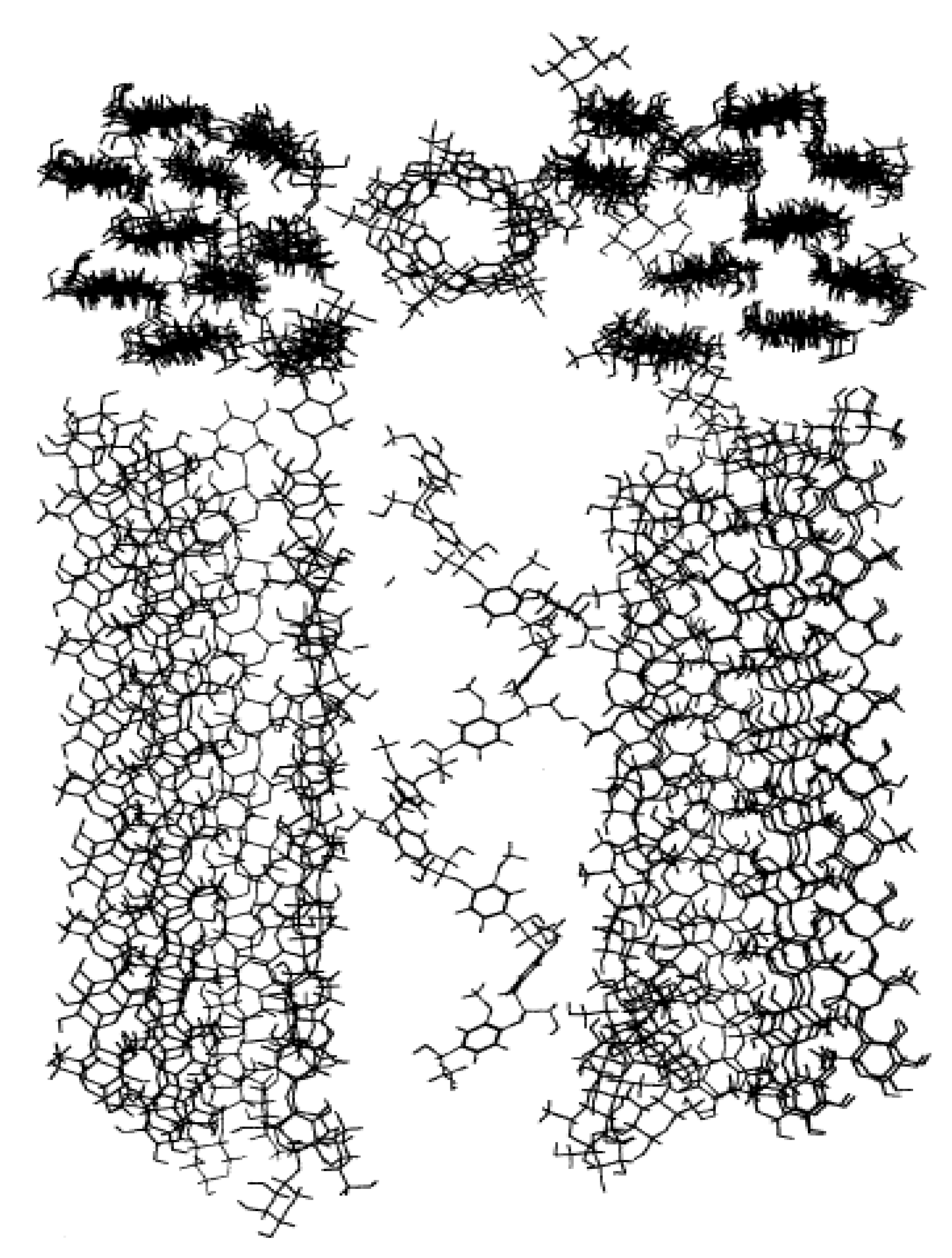
Faulon et al. [20] carried out one of the first successful simulations of lignocellulosics in gymnospermous wood. They used the DREIDING force field for most of the simulations. DREIDING is a 1st generation force field with the specifics reported in [7]. 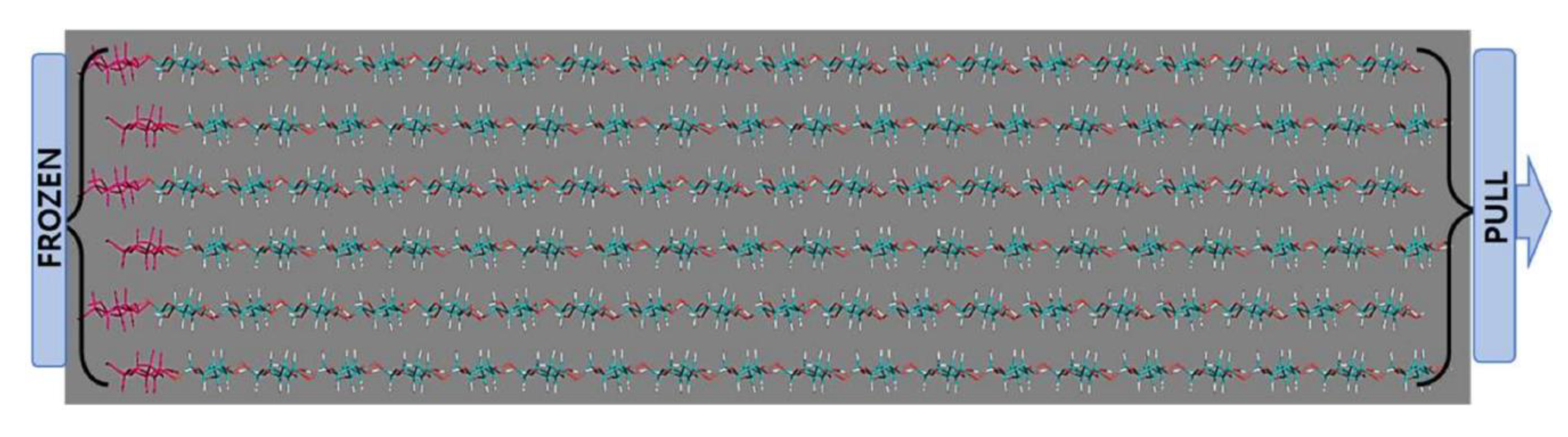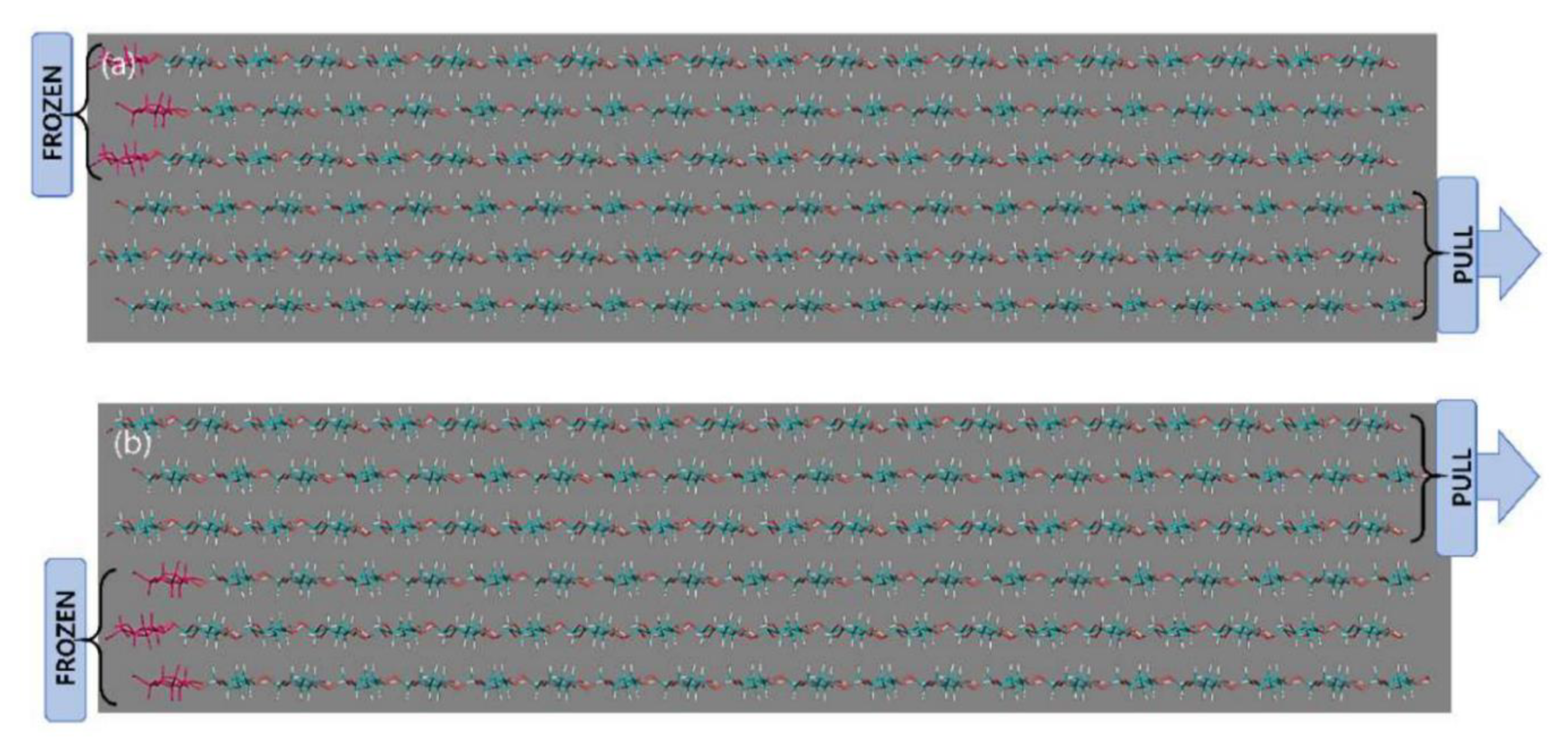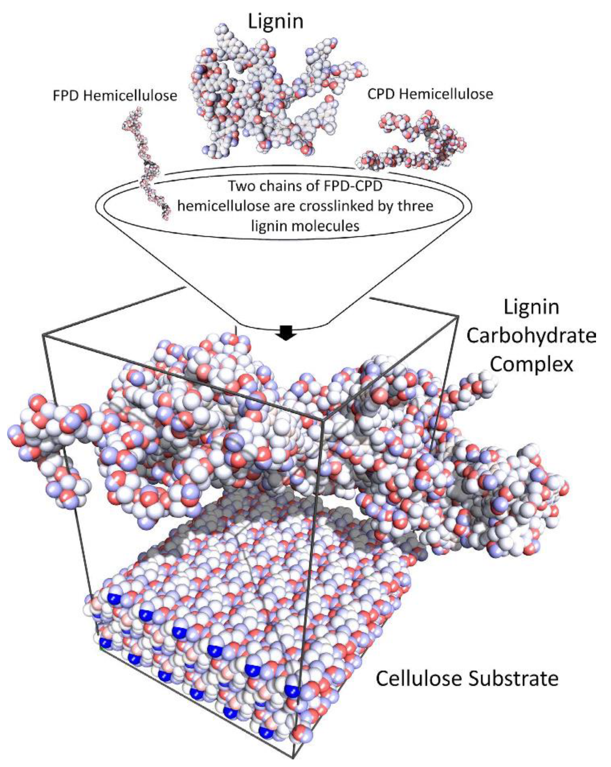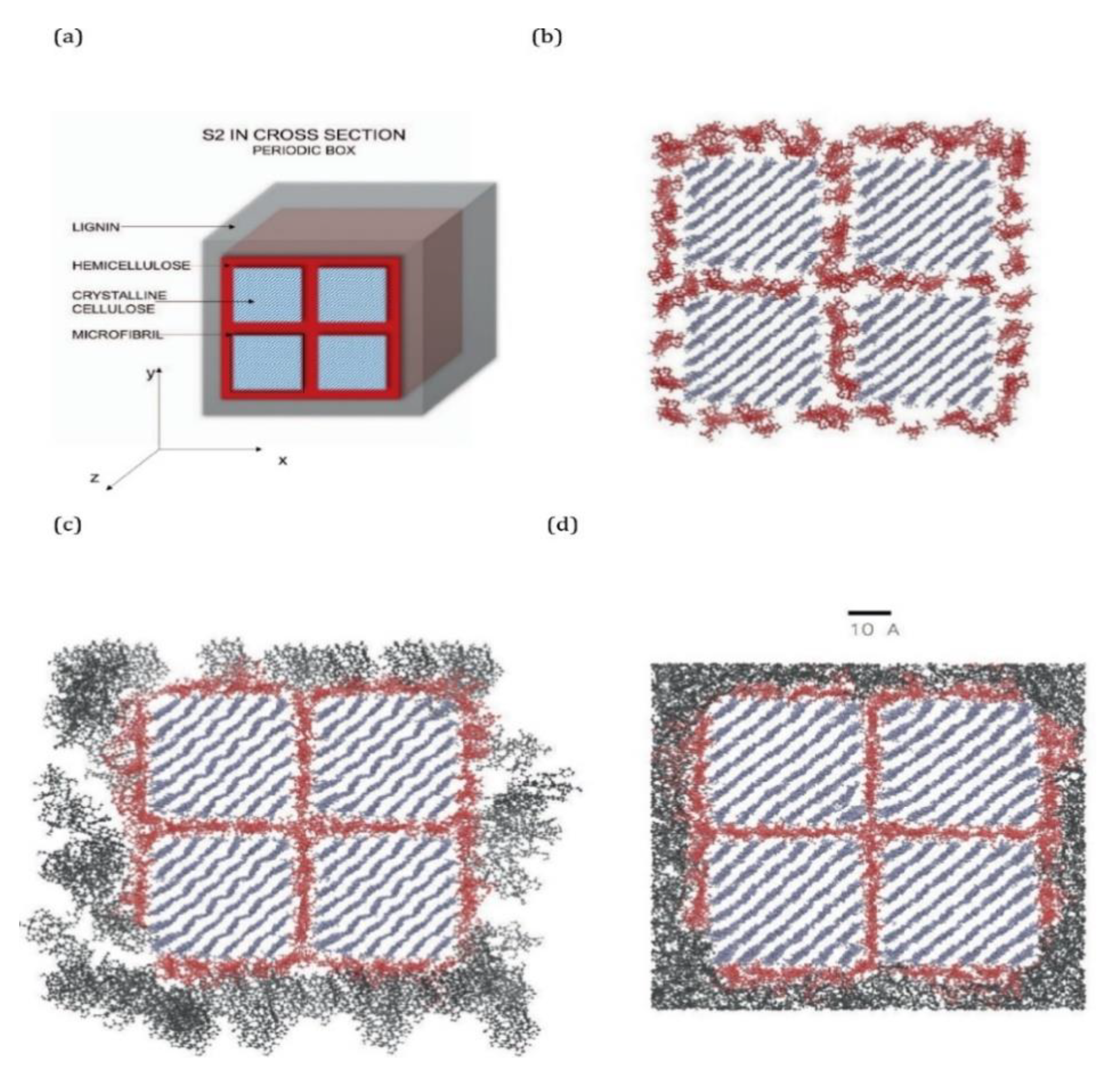The simulations were carried out at 300 K and for a relatively small length ranging from 120 ps to 240 ps owing to the capabilities of the time (ca 1994) but were still able to determine profound structural information about lignocellulosics within the cell wall of gymnospermous wood [20]. They constructed the lignocellulosic model (Figure 2) by incorporating 1 out of 4 separate lignin units within a polysaccharide unit comprised of cellulose chains and hemicellulose layers (Figure 2).

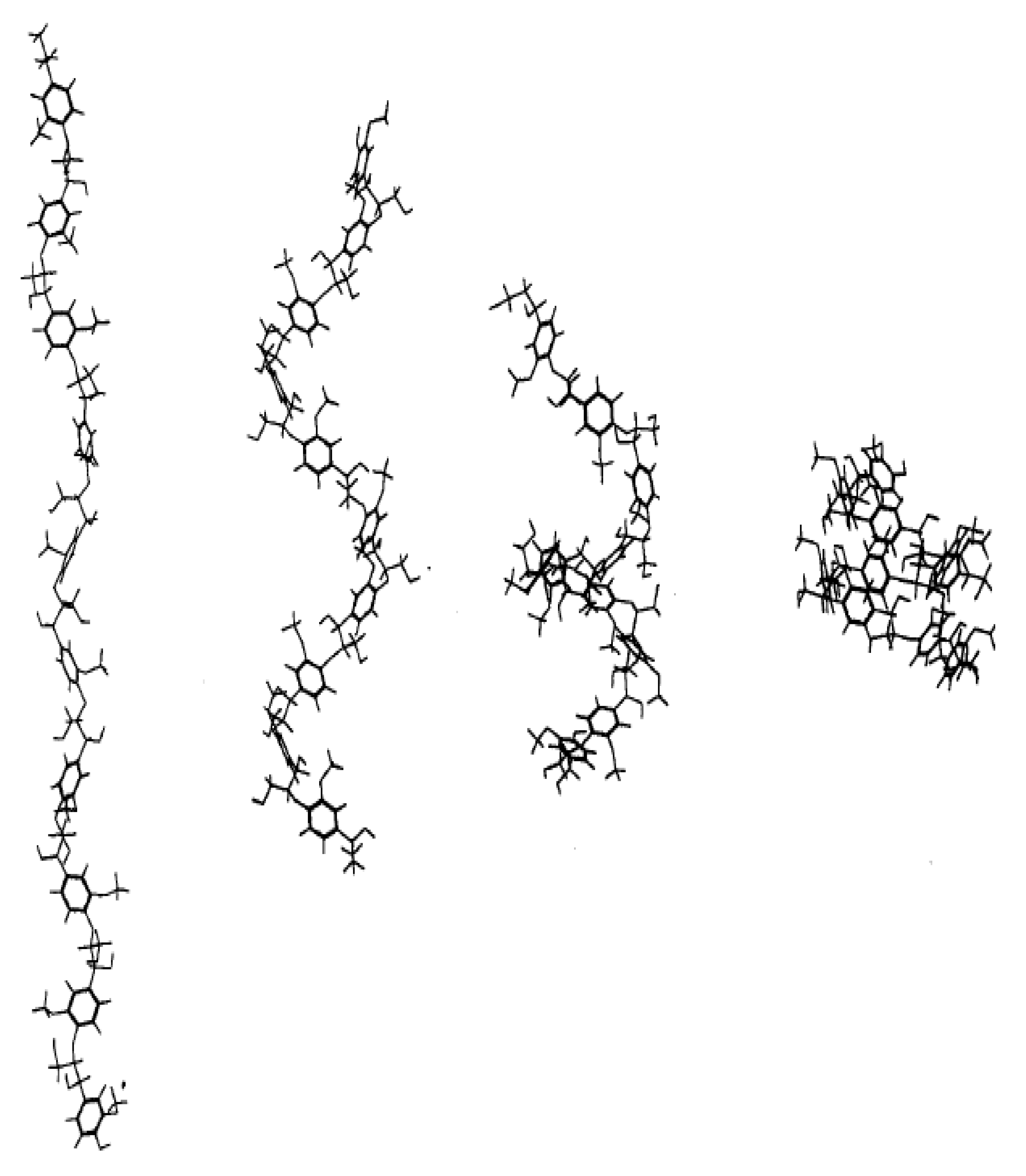
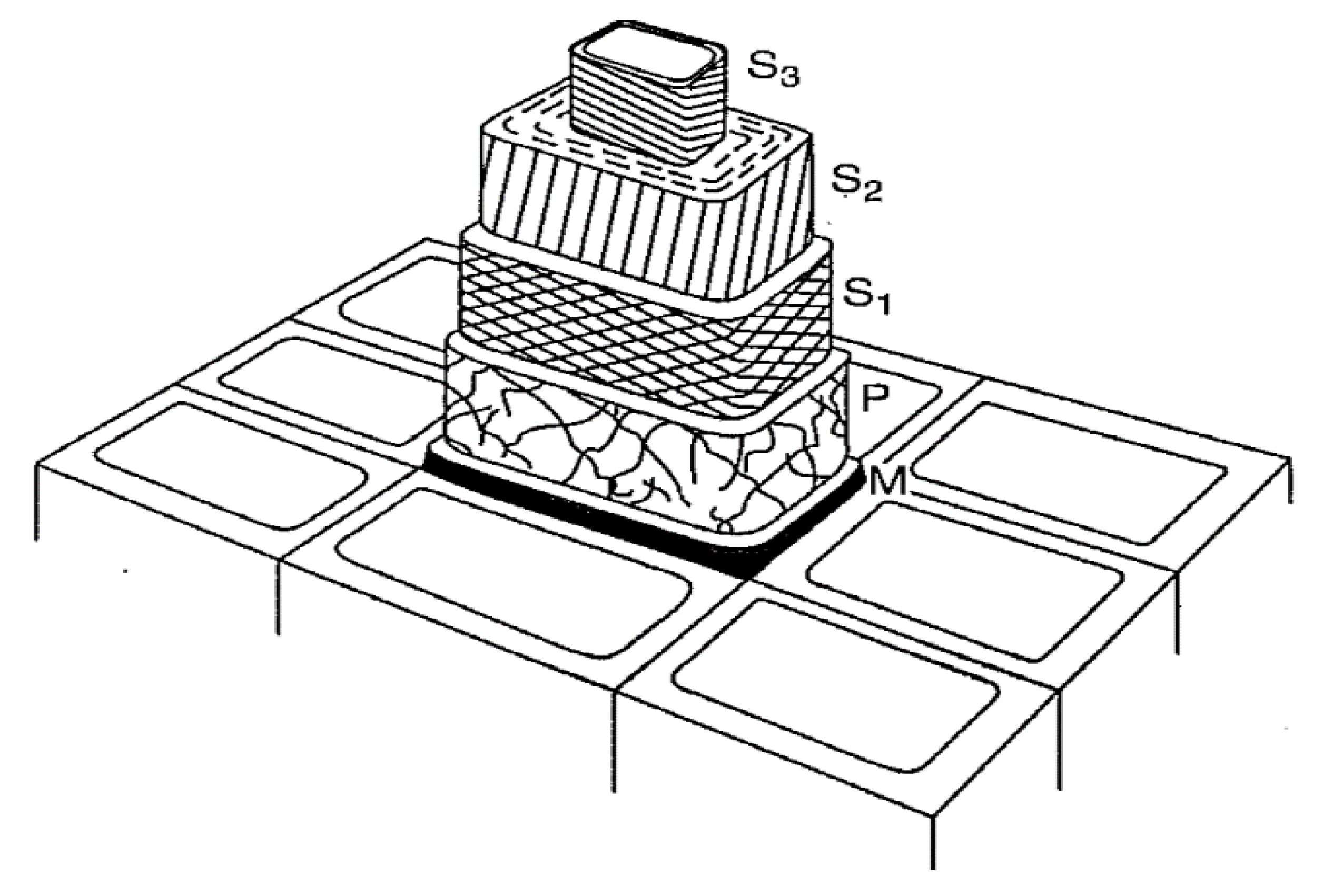
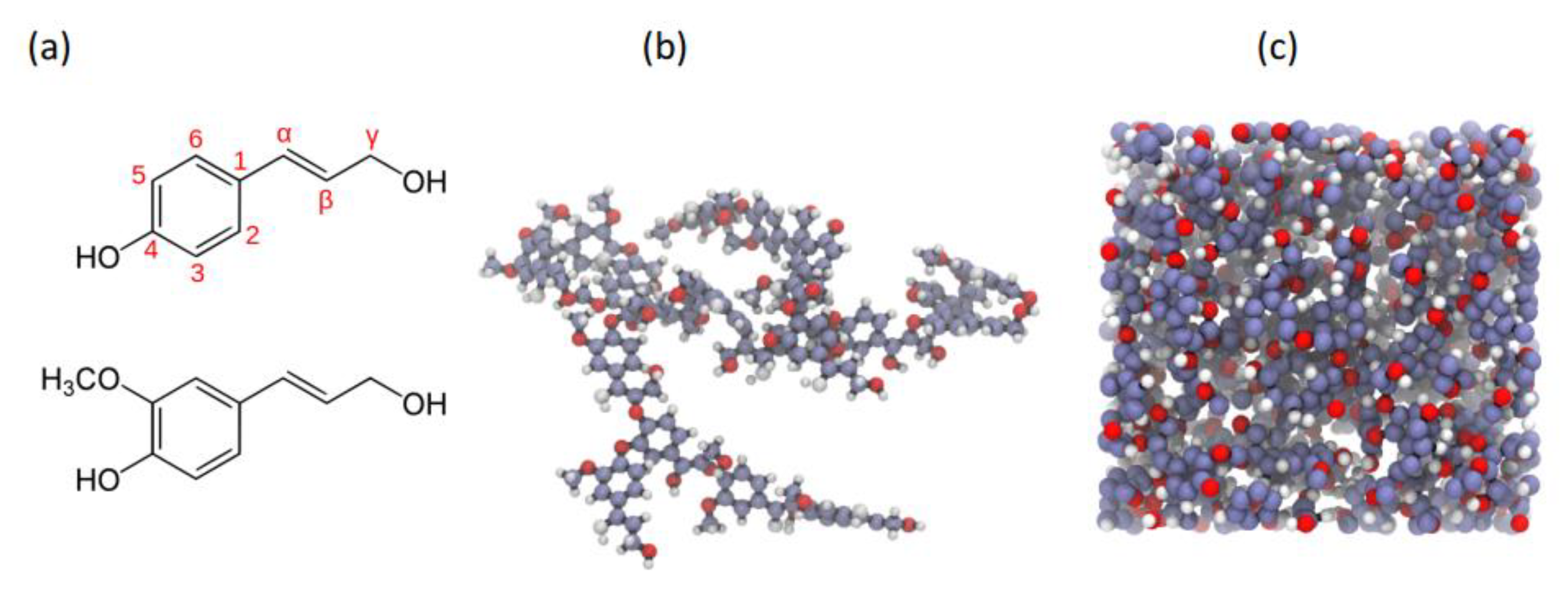
The lignin and hemicellulose were allowed to move during the MD simulation while the cellulose chains were fixed in place to approximate the crystalline I structure of cellulose within the cell walls of wood. The observations made by Faulon et al. [20] showed that the lignin structures evolved to form hydrogen bonds with the hemicellulose chains and cellulose chains. Hydrogen bonds were present between the α and γ alcohols of the lignin and the alcohol functional groups of the different sugar units. The presence of hydrogen bonds between lignin and polysaccharides causes each lignin structure to retain its initial conformation. When lignin is associated with polysaccharides as in the secondary cell wall, the helical structure is probably elongated (as the first structure in Figure 3) due to limited space between microfibrils and is also influenced by the crystallinity of the microfibrils. However, in portions of wood cells poor in polysaccharides such as the compound middle lamella, the structure is not supported by cellulose chains and is free to collapse to the most stable conformation-structure (as the last structure in Figure 3).

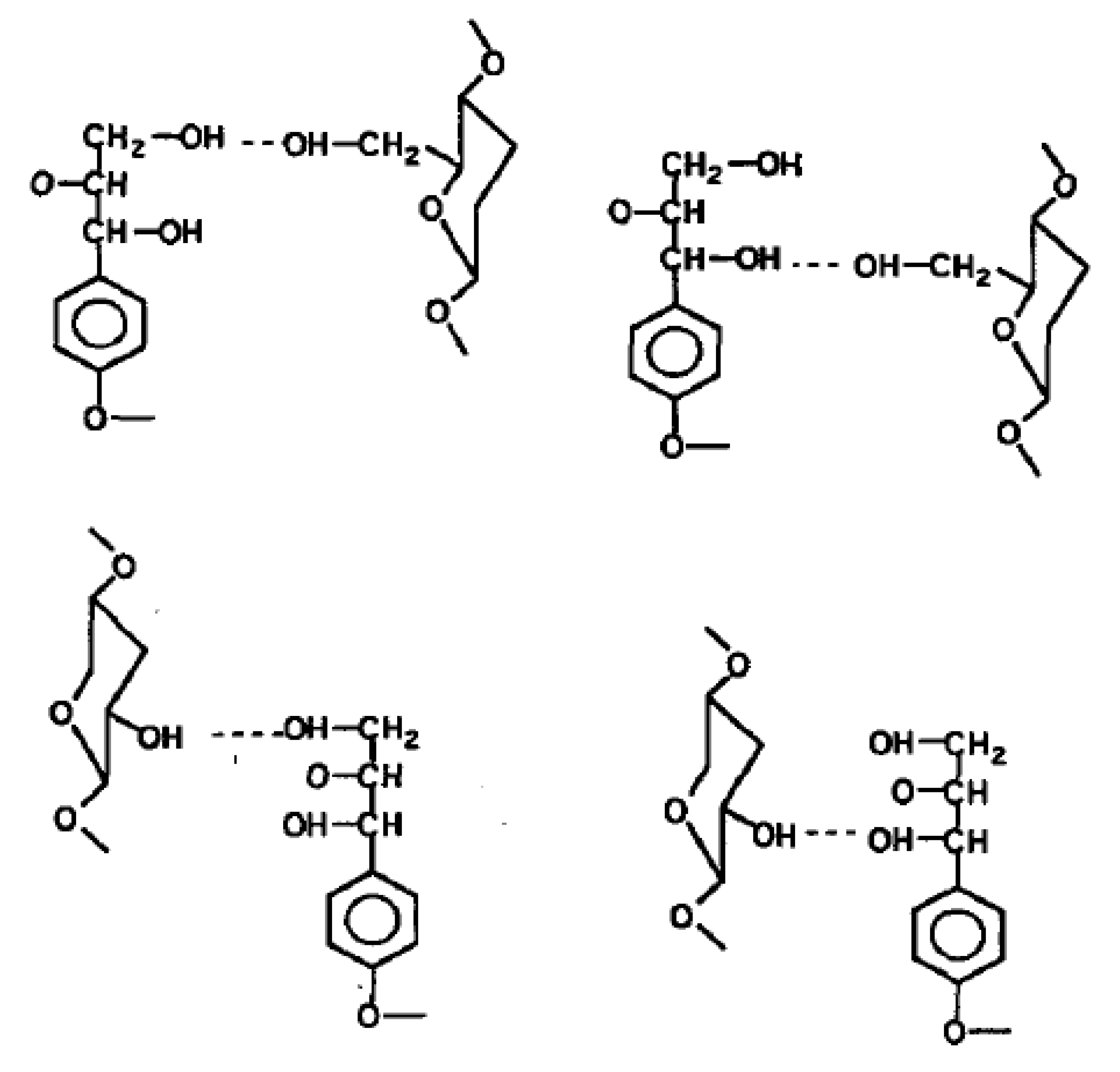
Faulon et al. [20] also indicated the four possible sites for hydrogen bonds between lignin and polysaccharides in Figure 4. While critical molecular information was obtained from their work, Faulon et al. [20] did not determine any physical/mechanical properties of the lignocellulosics.

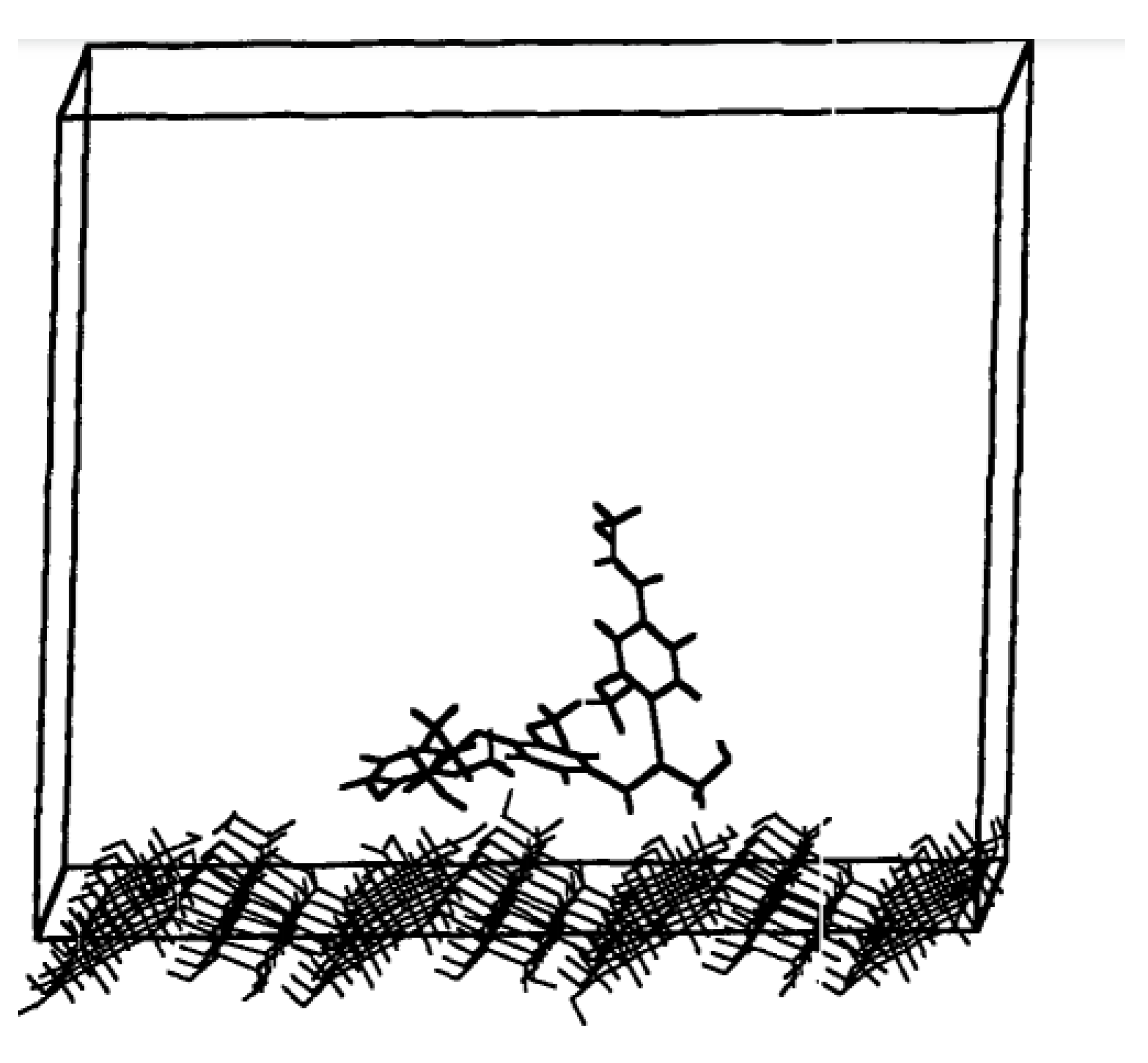
Houtman and Atalla [21] expanded upon the work of Faulon et al [20], using the consistent-valence forcefield (CVFF) for a similation time of 400 ps at 300 K and a cut off distance of 13 Å to model the interactions between a model lignin (coniferyl alcohol) compound with cellulose/polysaccharide surface. An illustration of the computational model used by Houtman and Atalla [21] is shown in Figure 5. It was found that two of the phenyl rings of the coniferyl alcohol are closely associated with the surface, but the third continued to remain free from strong associations with the surface. The adsorption of this third phenyl ring appears to be inhibited by the constraints of the β-O-4 linkage. Analysis of the cellulose surface showed that the lignin model was adsorbed over a region of high concentration of hydroxyl groups. This suggested that the dominant force holding the lignin model on the surface is electrostatic dipole–dipole interactions.

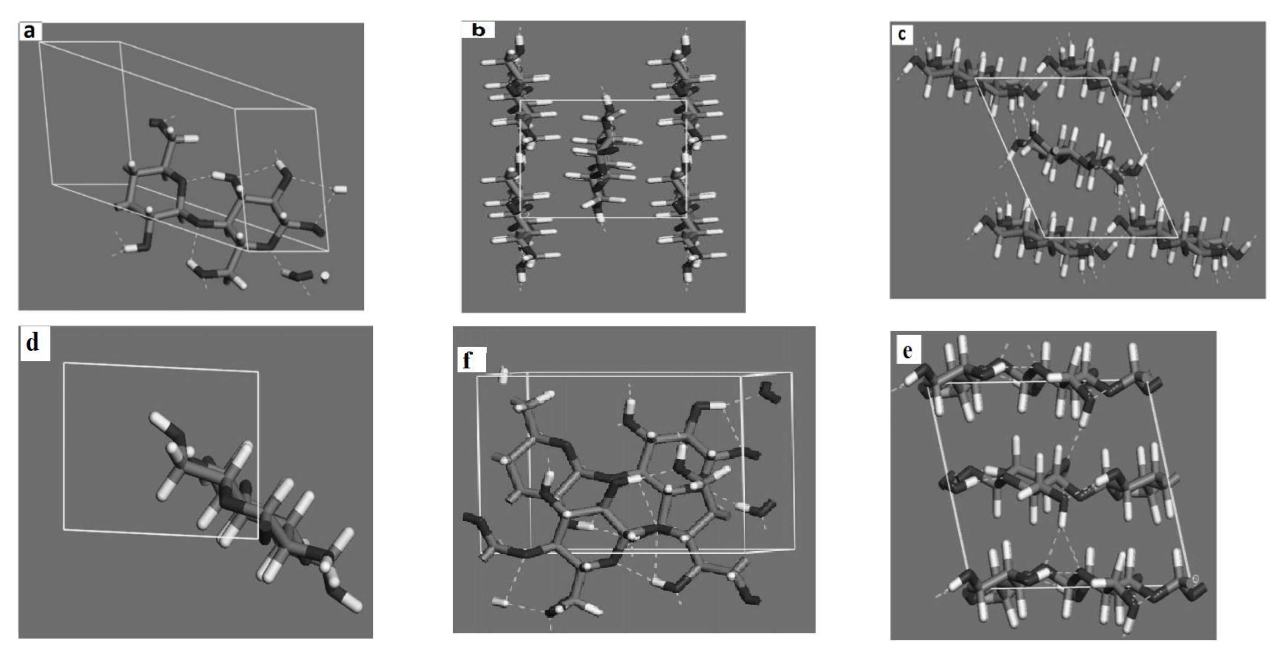
The CVFF was also used by Ganster and Blackwell [22] in one of the first attempts to simulate crystalline polymorphs of cellulose (Figure 6). The simulation was done for a period of 540 ps using the Verlet method [4] and a cut off of 9.5 Å at a starting temperature of 602 K which was slowly cooled to a target temperature of 298 K. No analysis was conducted regarding the thermal stability of the starting configuration at 602 K. Following the MD procedure, they found that there was a strong anisotropy for shear along the chains. In planes containing the chain axis, the shear modulus ranged from 5 to 20 GPa. Structural properties of the simulated cellulose were favourably comparable to real experimental data obtained through x-ray diffraction as shown in

Table 1. Experimental validation of MD data for Cellulose. With permission from.

Cell Dimension	Experimental Data from X-ray Structural Analysis	MD Data from Ganster and Blackwell [22]
a (Å)	8.01	7.80
b (Å)	9.04	9.31
c (Å)	10.36	10.74
α (°)	90	90
β (°)	90	90
γ (°)	117.1	116.6
Density (g/cm3)	1.61	1.54

.

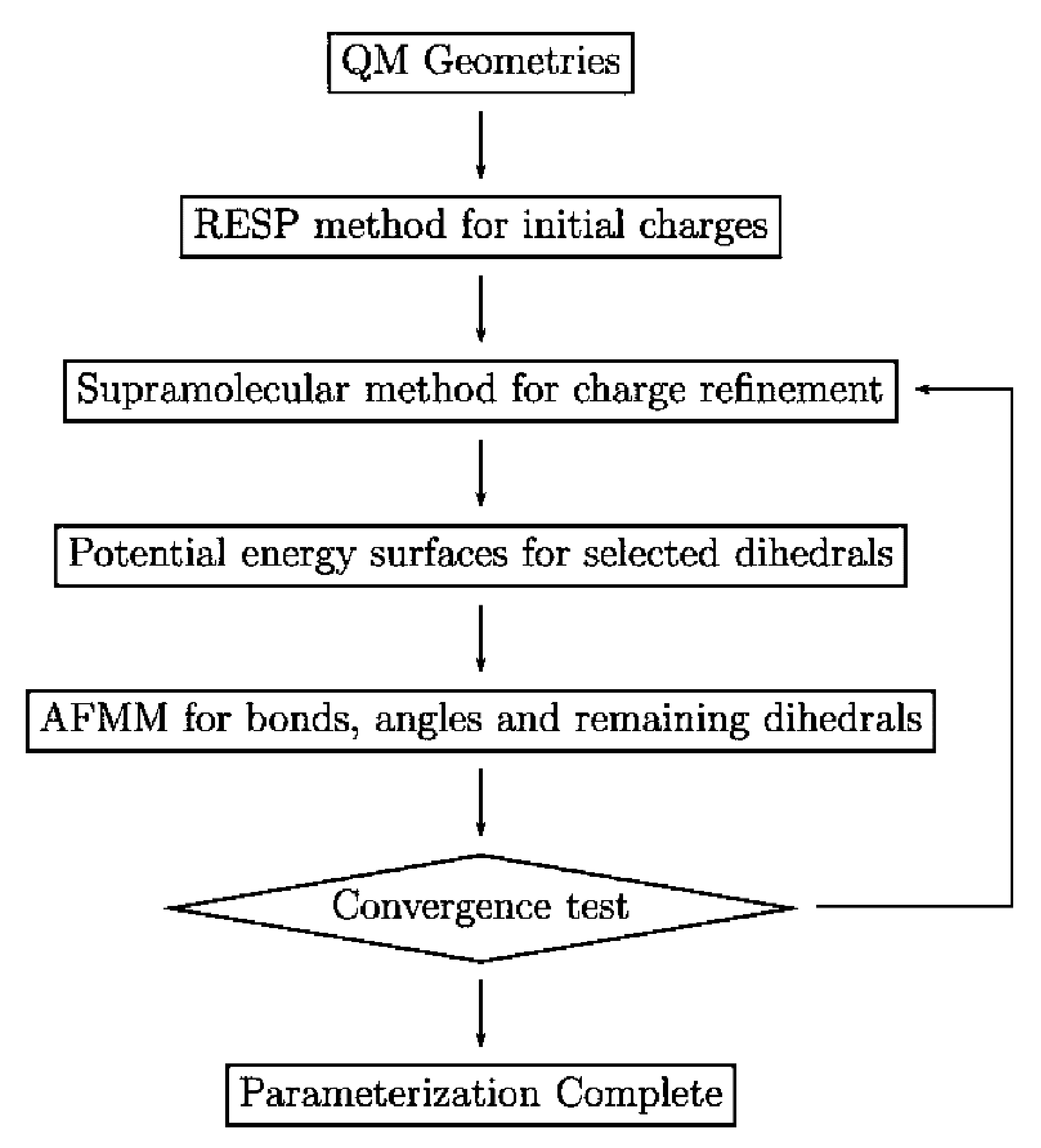
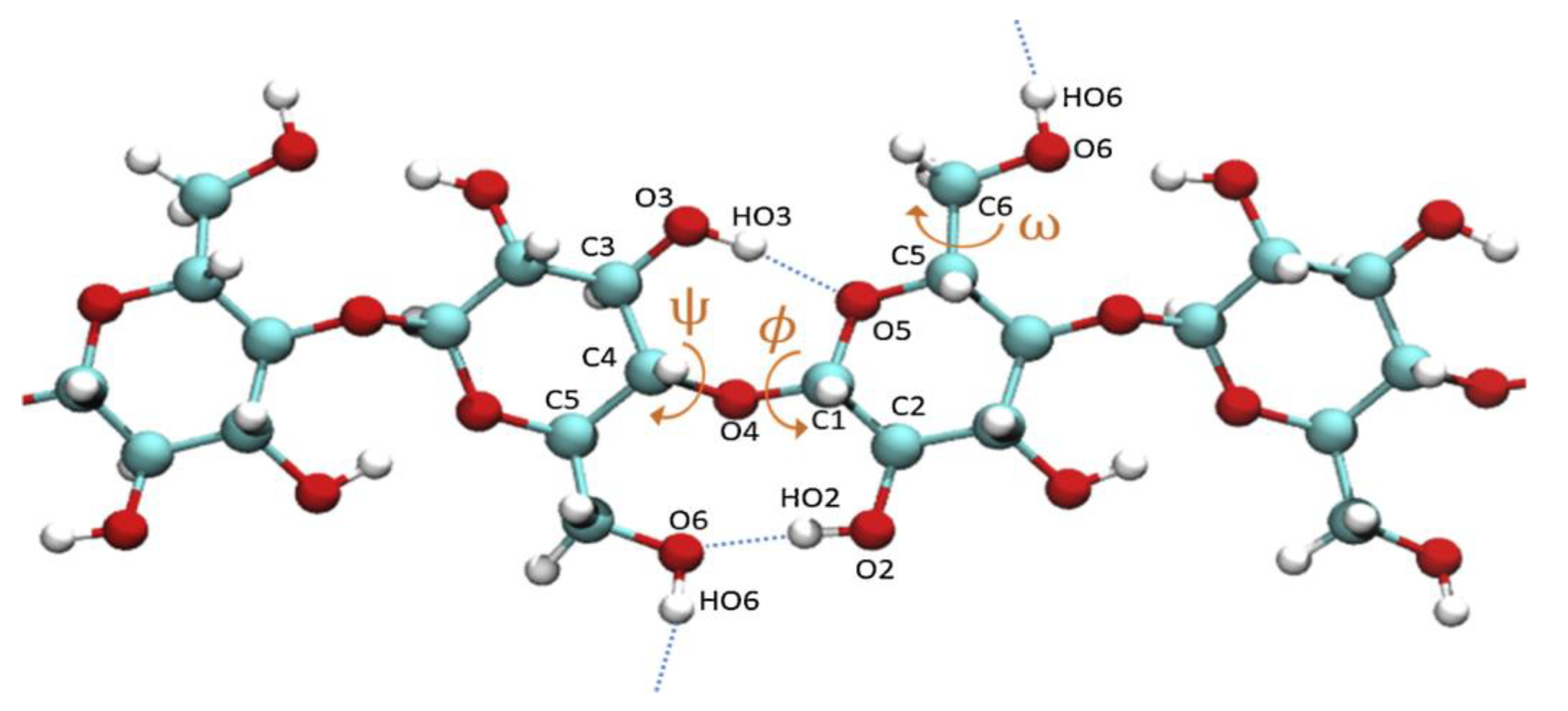
The MD algorithm developed by Petridis and Smith in [23] involved optimization of the electrostatic interactions by assigning partial atomic charges so as to reproduce quantum chemical data. These charges were taken into account to ensure the presence of electronic polarization within the context of condensed phase simulations. Dihedral force constants were determined by examining potential energy surfaces. The interactions between bonded atoms were subsequently optimized with respect to quantum chemical vibrational data using the Automated Frequency Matching Method developed by Vaiana et al. [24]. It was found that dihedral rotations around the β-O-4 linkage within the lignin structure played a significant role in determining the configuration of the lignin macromolecule [25,26]. Petridis et al. studied two equivalent dihedrals in lignin model system for showing the dihedral rotations [23]. 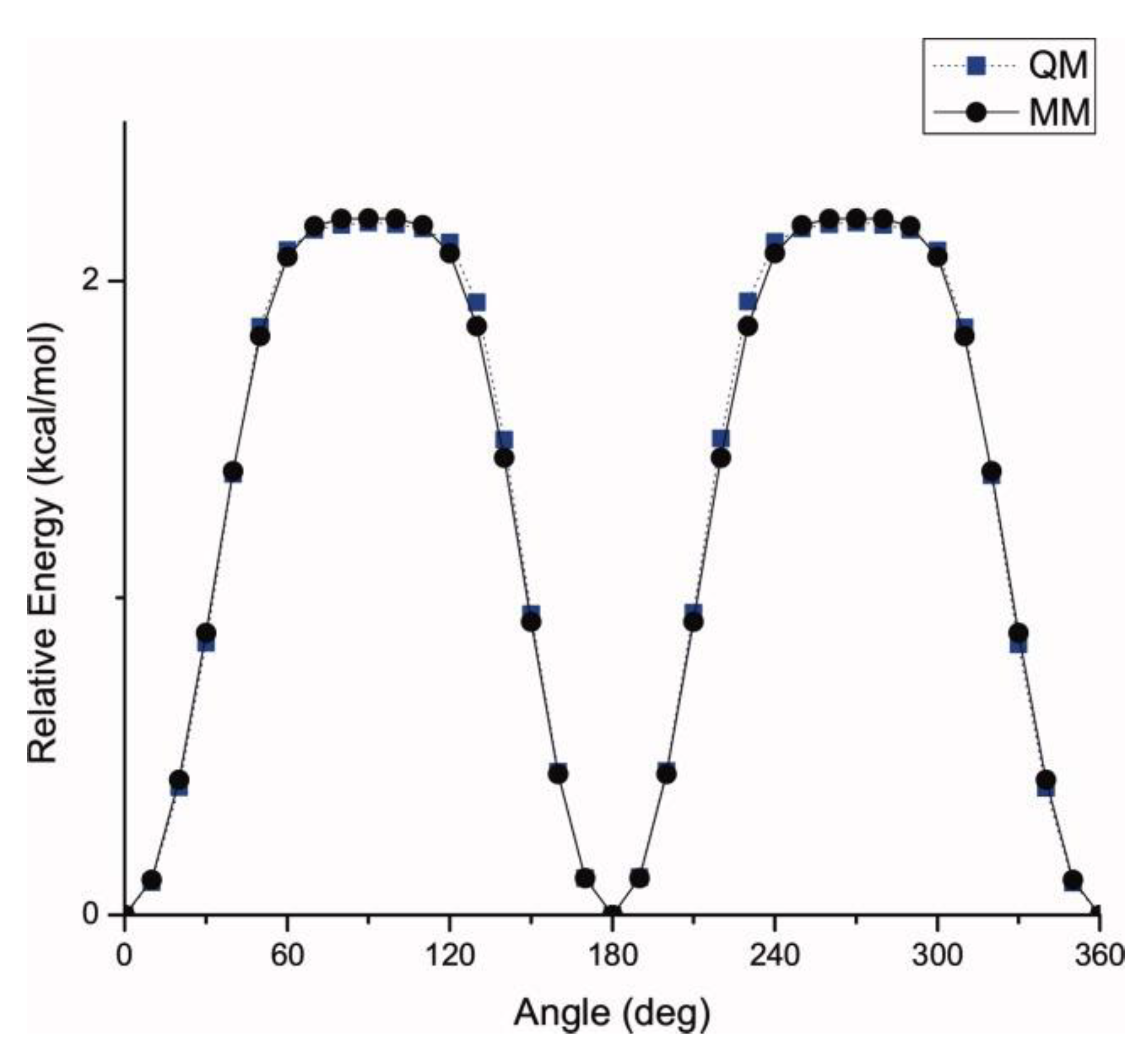These are ω₁: C₂-C₁-O-C_α (or C₆-C₁-O-C_α equivalently) and ω₂: C₁-O-C_α-H. They observed that the molecular rotation around these dihedrals leads to severe steric hindrance between the two aromatic rings of guaiacyl and syringyl units connected with β-O-4 linkage. As an example, the comparison between the quantum mechanical and force field predicted dihedral rotations of anisole model are shown in Figure 7. The predictions were obtained using a parameterization process shown in Figure 8.

The dihedral rotations around the β-O-4 linkage of lignin structure confirmed the conjecture of Faulon et al. [20]. In a separate study, the influence of intramolecular H-bonding on the dynamical conformational behaviour of the β-O-4 structure was studied to support the theoretical data. In this study, the experimental NMR data clearly indicated that the guaiacyl β-O-4 structure experiences conformational changes in solution and the intramolecular H- bonds to solvent molecules predominate. This study concluded that the guaiacyl β-O-4 structure is flexible and intramolecular H-bonds are not strong and persistent enough to confer rigidity to the molecule in solution. 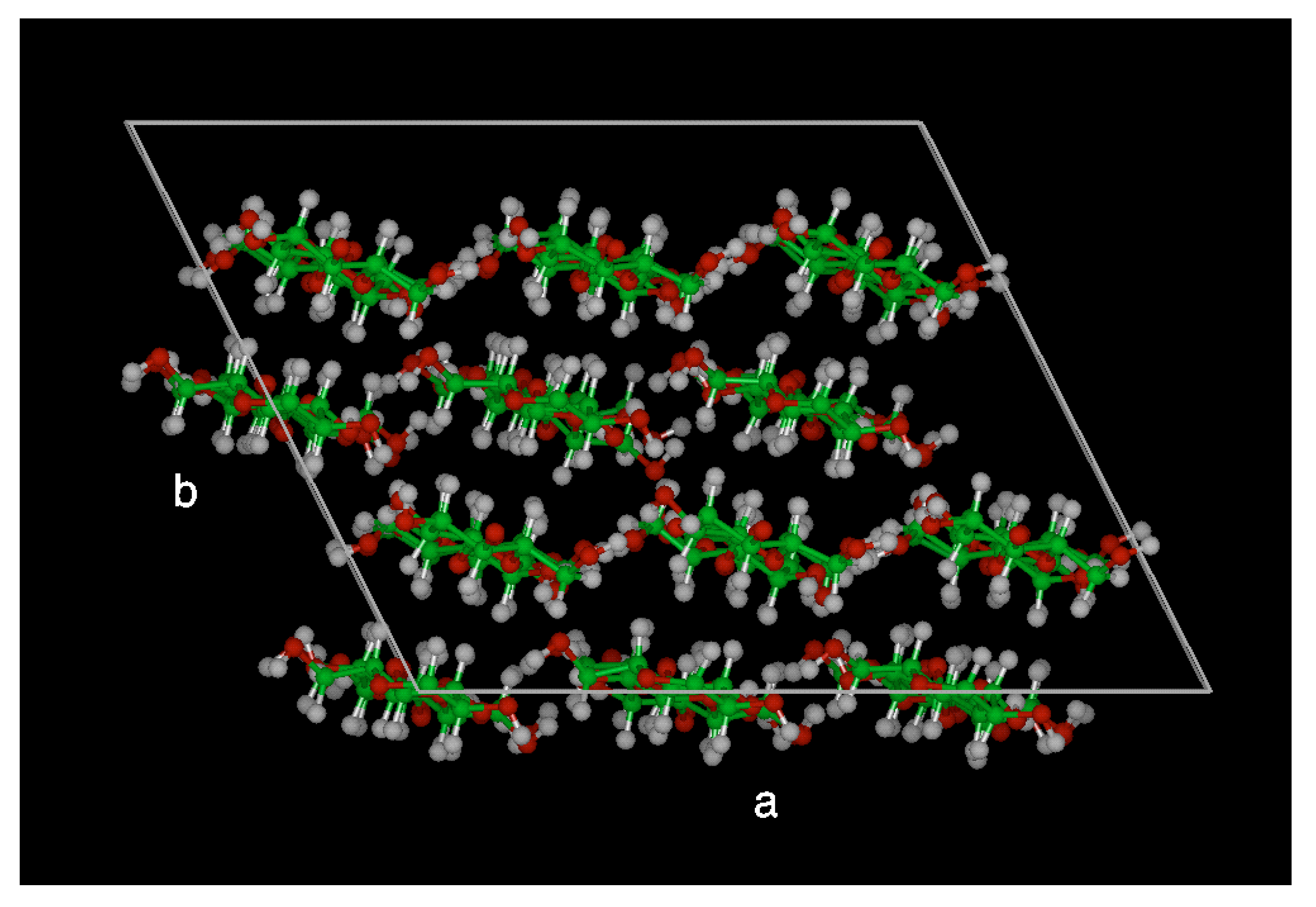This concept was verified via both molecular modelling and NMR study [28,29]. The specific parameterization of the force field was done using two model compounds- anisole and 4-(1,2,3-trihydroxypropyl) phenol (PHP). To establish the validity of the developed molecular mechanics force field, the crystal structure of a lignin sub-unit dimer, erythro-2-(2,6-Dimethoxy-4-methylphenoxy)-1- (4-hydroxy-3,5-dimethoxyphenyl) propane-1,3-diol (EPD) was used. EPD is very similar to two syringyl units connected with a β-O-4 linkage, but with the hydroxy group of one of the phenol rings substituted by a methyl group. The excellent agreements between the MD and experimental data as regards the physical (in this case, crystalline) properties of EPD is shown in

Table 2. Experimental validation of MD data for EPD. With permission from [23].

Cell Dimension	Experimental Data	MD Data from Petridis and Smith [23]
a (Å)	8.69	8.73 ± 0.02
b (Å)	8.90	8.93 ± 0.01
c (Å)	13.11	13.68 ± 0.03
α (°)	73.85	74.48 ± 0.05
β (°)	86.15	86.30 ± 0.01
γ (°)	83.06	83.06 ± 0.02
Cell volume (cubic Å)	966	1020

.

Fine structural characteristics of lignocellulosic materials also entails understanding the interactions between the individual lignocellulosic phases and the water molecules they exist in association with. Faulon et al. [20] were able to isolate the bonds/moieties in lignocellulosics that contribute most to the hydrogen bonding interactions but did not conduct any specific water-cellulose-lignin interaction simulations. The water molecules that form an intrinsic part of the lignocellulosic network. Therefore, when it comes to understanding lignocellulosic behaviour, it is fundamental to take into account the dynamics of these water molecules when they are in contact with the lignocellulosic material. To study the dynamics of the bound water with cellulose, O’Neill et al. [30] utilised a MD based approach and validated the simulations using quasi-elastic neutron scattering (QENS). In a previous work, Petridis et al. [31] had shown how cellulose was found to be more rigid in the hydrated state than in the dry state, and evidence was found that in hydrated cellulose the cellulose chains are more closely packed and water molecules bridge the chains through hydrogen bonding interactions.

The molecular model used in [30] contained four aligned cellulose (cellulose Iα) microfibrils. Each microfibril contained 36 chains with a degree of polymerization of 80. The system was solvated at 0.20 g water/g cellulose to match the experiments. The simulations were performed employing the GROMACS software [11] and a parameterised CHARMM C36 carbohydrate force field similar to [27]. The TIP4P water model was chosen for simulating the water molecules owing to the derived self-diffusion coefficient being in good agreement with experiments. Periodic boundary conditions were employed together with the Particle Mesh Ewald (PME) algorithm and an interaction cut-off distance of 12 Å for electrostatics and between 9 and 10 Å for the van der Waals interaction to reduce computational requirements. Each system was simulated for a total of 11 ns at three temperatures: 213 K, 243 K and 263 K and at atmospheric pressure. The data from the final 5 ns of each simulation were analysed, once the system had reached equilibration. This methodology, where the initial non equilibrium simulation data is discarded and the final few ns post equilibrium is only taken into account, was utilised for estimating diffusion coefficients in semicrystalline polymer-lignocelluosic composites by Prasad et al. [32,33]. In [32,33], semi empirical multiphase modelling was used to further increase the accuracy of the simulated data combined with the use of the PCFF (Polymer Consistent Force Field) for MD simulations. O’Neill et al. 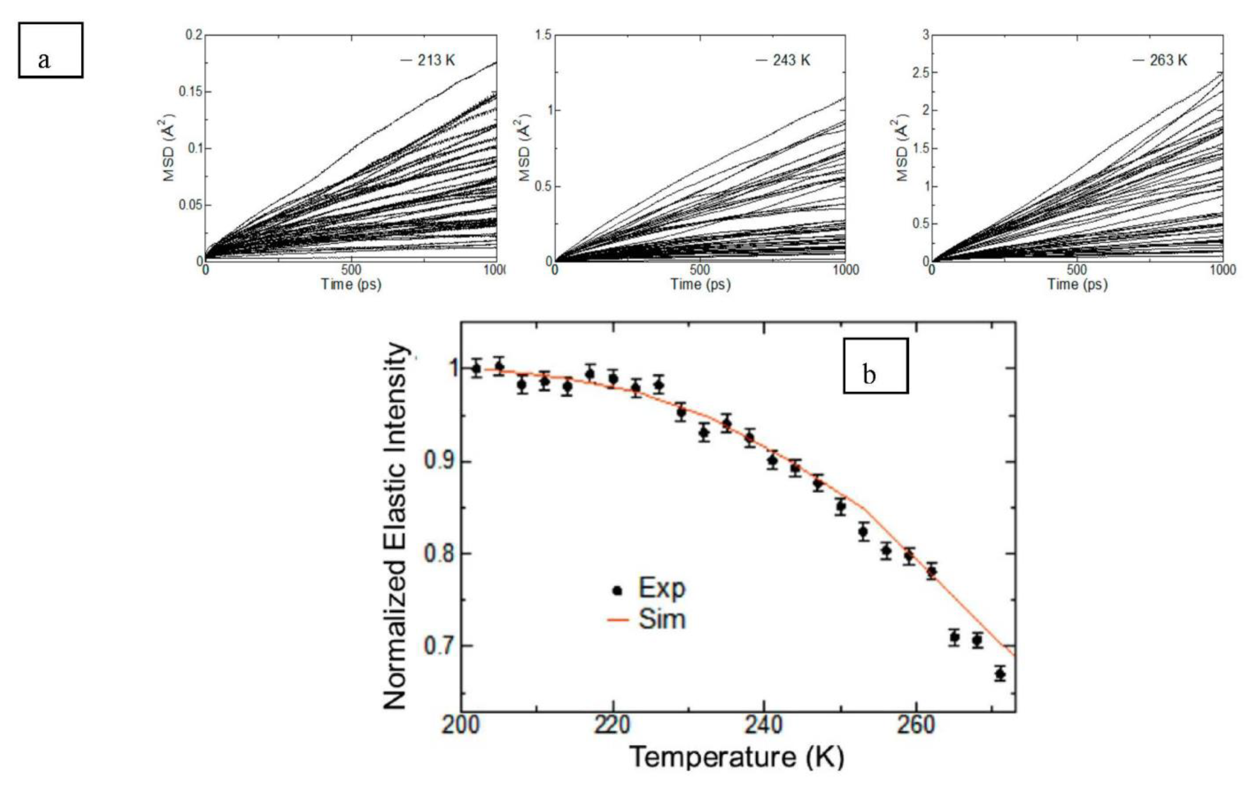[30] in Figure 9 correlated the elastic intensity ‘S_el (T)’ at a temperature ‘T’ for the neutron scattering wave vector ‘Q’ to the mean squared displacement/MSD (${\mathsf{\Delta }\mathrm{r}}^2$) of the bound water molecules using the Gaussian approximation given by Equation (18). Using the Einstein relationship also used by Prasad et al. [32,33] amongst others, the MSD could then be used to estimate the diffusion coefficient D.

$${\mathrm{S}}_{\mathrm{el}}\left(\mathrm{T}\right)\propto { \mathrm{e}}^{\frac{-{\mathrm{Q}}^2{\mathsf{\Delta }\mathrm{r}}^2}{3}}$$

(18)

As seen from Figure 9b, an excellent agreement was found between the calculated and measured MSD showing that the simulated system was very accurate in terms of estimating the dynamics of water in real crystalline cellulose. O’Neill et al. [30] stated that the knowledge of such dynamical properties of bound water in lignocellulosic systems and the partition behaviour of the bound water in the cellulose supramolecular structure could further enhance the understanding of water’s role in the change of biomass morphology during different pre-treatment regimes for biofuels production. This can potentially lead to more efficient pre-treatment approaches.

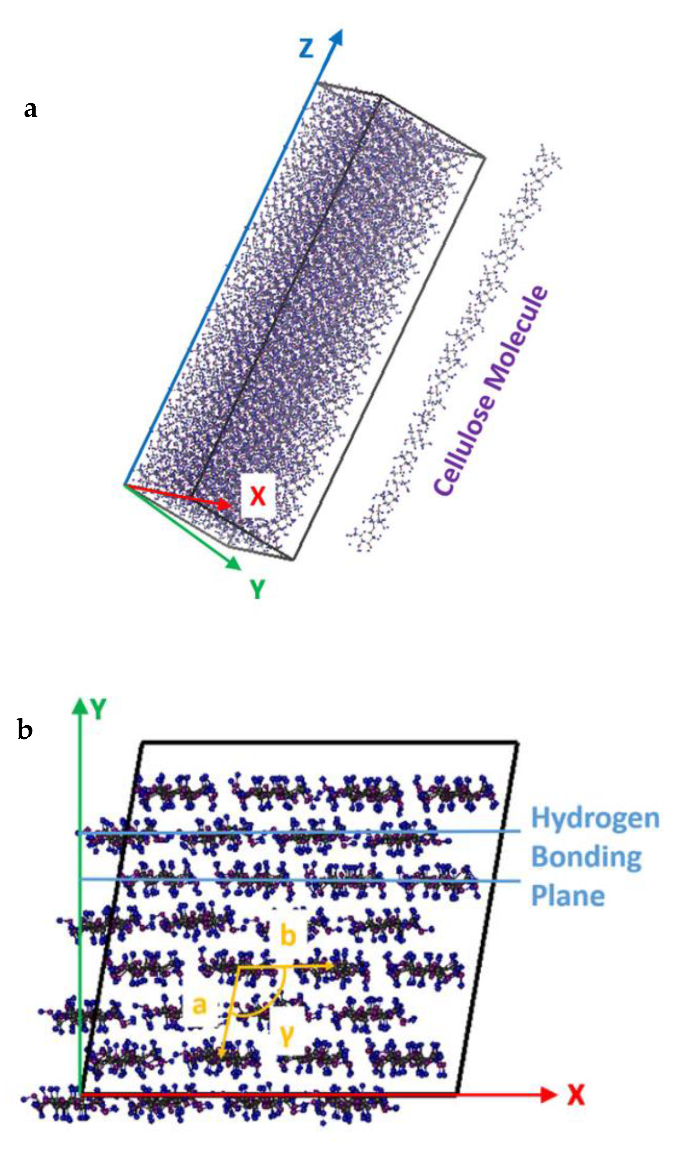
Bound water dynamics was then correlated to the molecular orientation of the cellulose molecules by Petridis et al. [31]. Similar to [30], the simulated system contains four aligned cellulose Iα fibres, the predominant allomorph of bacterial cellulose, each consisting of 36 chains with a chain length of 80 glucose monomers. The shape of the fibres is “diamond”, with the hydrophilic (100) and (010) crystallographic faces predominantly exposed to the solvent in this case, water and the interaction of water with cellulose hydrophilic and hydrophobic surfaces was studied. The simulated fibres were studied at dry and at hydrated conditions (0.20 g of water per g of cellulose). The parameterised CHARMM C36 carbohydrate force field was once again used for the cellulose and the TIP4P-EW model was used to simulate the bound water molecules. The simulations were performed with the program GROMACS [11] using a time step of 2 fs. Bonds involving hydrogen atoms were constrained using the LINCS algorithm (fourth order with one iteration), and for water the SETTLE algorithm was used. Periodic boundary conditions were employed, and the PME algorithm [31] was used for electrostatic interactions. A cut-off of 12 Å was used for the electrostatic interactions and 9−10 Å for the van der Waals interactions. Each system was simulated at a pressure of 105 Pa and at 16 temperatures: from T = 153 to 293 K in 10 K increments and at 298 K. Simulations were 11 ns long with data from the last 10 ns of simulation at each temperature being analysed similar to [31,32,33].

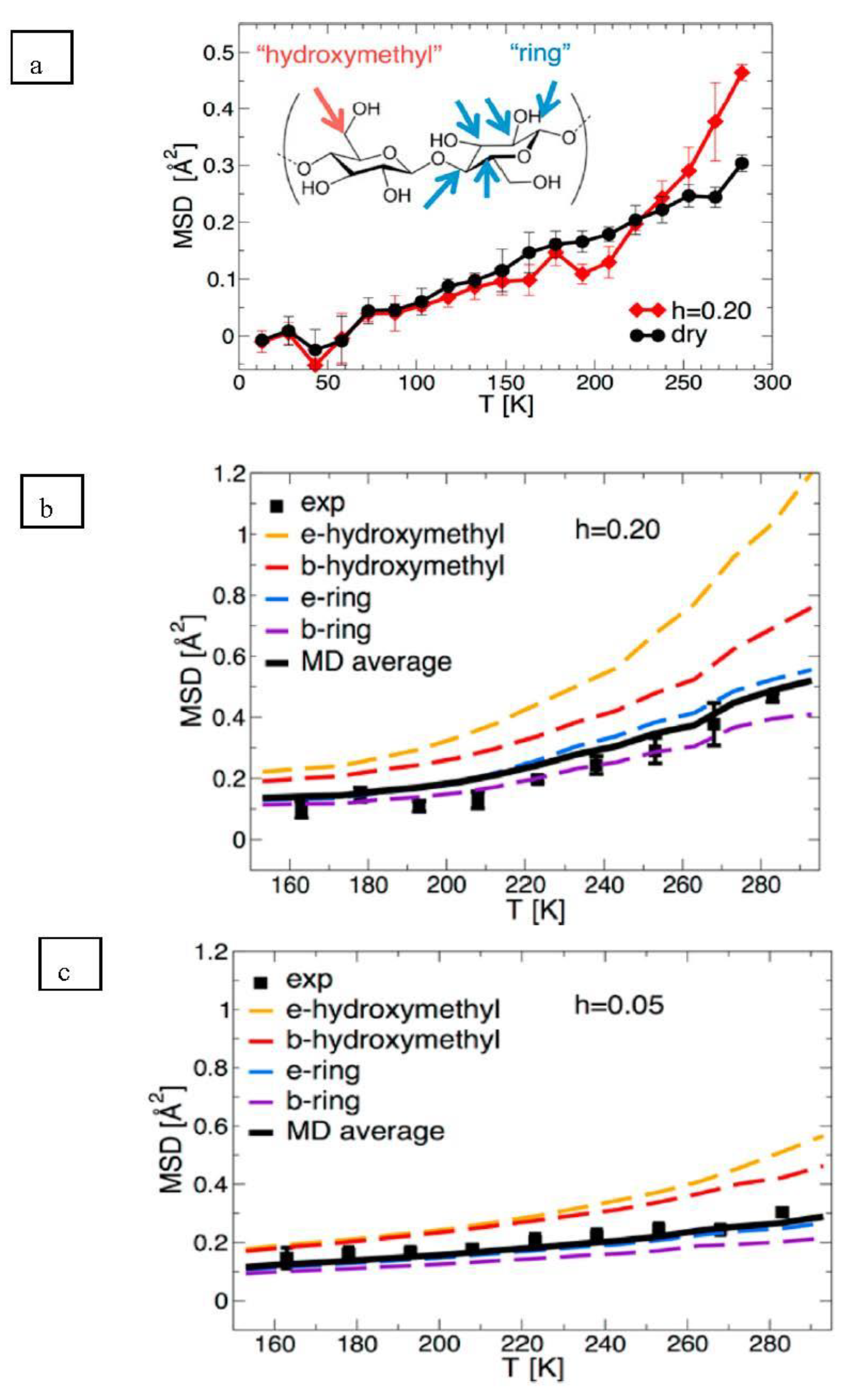
The experimental atomic MSD, a quantitative measure of the average magnitude of atomic motions, of the two cellulose samples is shown in Figure 10. Up to ∼210 K both dry and hydrated cellulose display a relatively small increase in their MSD, indicating the underlying atomic fluctuations are not affected by hydration. However, a dynamical transition, indicated by a steep increase of MSD at T > 210 K is observed only in the hydrated sample (Figure 10a). This transition arises from the onset of large-amplitude, anharmonic dynamics. The simulation-derived MSD was then decomposed by Petridis et al. [31] into contributions from water-exposed or surface (“e-”) and water-buried or core (“b-”) hydroxymethyl and chain atoms in Figure 10b,c for the hydrated and dry cellulose simulated systems respectively. In all simulations, the MSD of the hydroxymethyl hydrogens was found to be always higher than that of the ring hydrogen atoms. Furthermore, those rings and hydroxymethyl hydrogens exposed to the water molecules (i.e., in hydrated condition) had higher MSD values than those in the core (Figure 10c). This indicated that there was a higher enhancement of molecular mobility upon hydration for the ring and hydroxymethyl hydrogens making up the surface groups relative to those groups in the core. A strong temperature dependence of the MSD is found only in the hydrated system and only for the exposed hydroxymethyl hydrogens, which account for only 1.5% of the total nonexchangeable hydrogen atoms in the entire system. In contrast, the average MSD of buried ring hydrogen atoms, which comprise 70% of the nonexchangeable H, is nearly independent of temperature. Therefore, the weaker experimental dynamical transition in cellulose relative to other biopolymers arises from the relatively small proportion of nonexchangeable hydrogens in the solvent-exposed side chain hydroxymethyl groups.

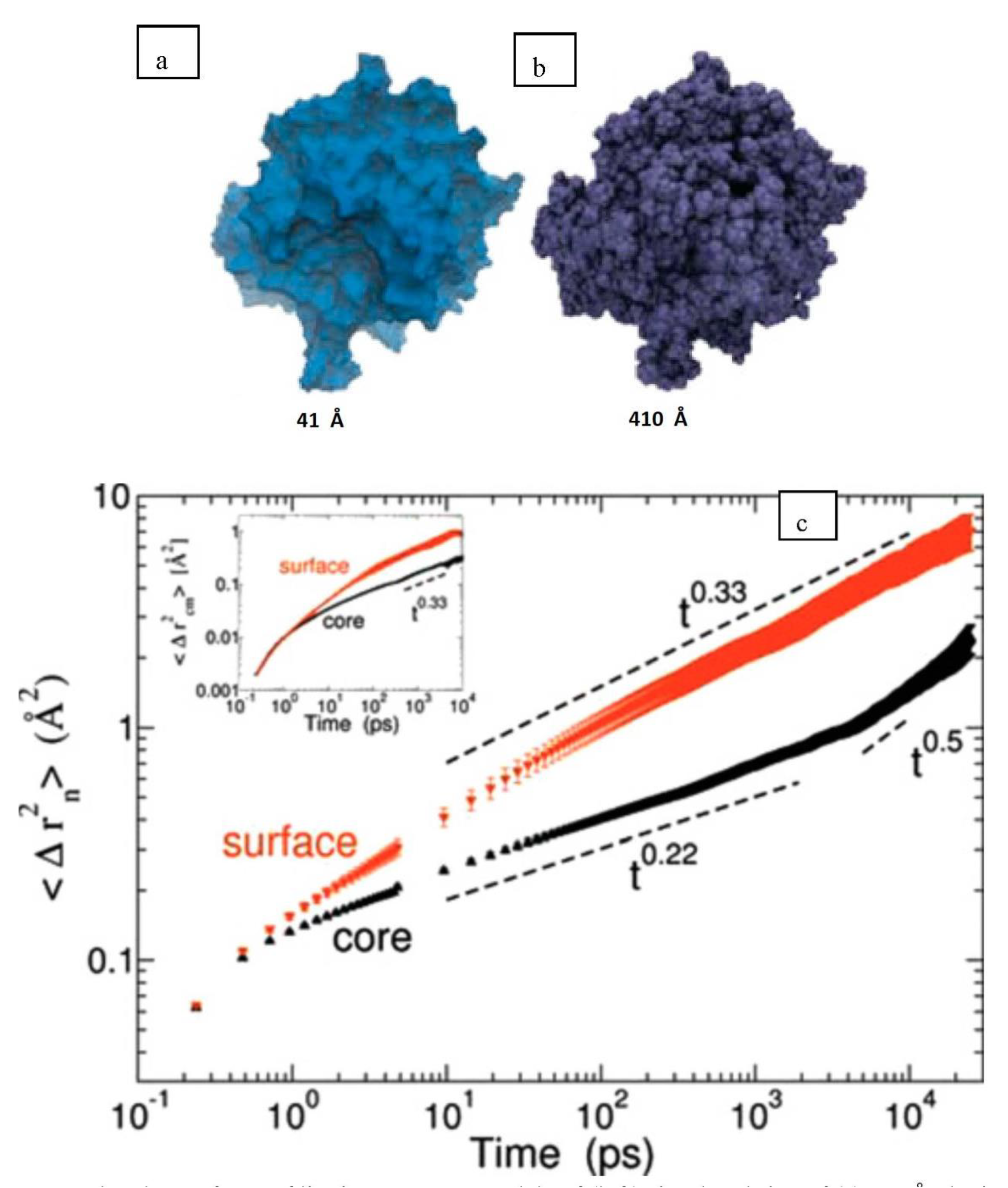
The higher enhancement of molecular mobility upon hydration of surface groups relative to those in the core was also found for lignin, another significant component of the lignocellulosic phase that comprises plant cell walls by Petridis et al. [34]. Simulated version of lignin aggregates, each with 25 13-kDa lignin polymers, were constructed and were simulated in similar hydrated conditions to [31] also using a parameterised CHARMM force field for lignin and the TIP3P water model. Extracted softwood (pine) lignin was first analysed using small-angle neutron scattering and an average aggregate size of up to 1300 Å was seen while the MD constructed models had a diameter of around 41 Å. To use MD to simulate true to life lignin models, Petridis et al. [34] suggested that at a scale of 1–1000 Å there is a scale invariance in both structure and behaviour of lignocellulosics. Therefore, a 410 Å (Figure 11b) aggregate was built using the 41 Å MD structure (Figure 11a). The MSD behaviour of the lignin molecules is then shown in Figure 11c and similar to semi crystalline polymers, seems to exist in 3 regimes viz., the ballistic regime (t ~ 0.1 ps), the confined/caged regime (0.1 ps < t < 5 ns) and the sub-diffusive regime (t > 5 ns). The second insight is that there exists a clear difference in MSD behaviour between the surface and core lignin molecules. Lignin monomers at the surface of the aggregate displayed considerably faster dynamics beyond the ballistic region (a four-fold increase of their MSD at t = 10 ns compared to the core monomers). This increase is also much more pronounced for the lignin as compared to the core and surface cellulose moieties as analysed in [31]. The higher crystallinities of the cellulose molecules as compared to the lignin molecules could be the reason for this, as crystalline polymers do show much lower MSDs than amorphous polymers at the same temperature. This was also established for diffusion of oxygen in crystalline and amorphous polyethylenes by Prasad et al. [32].

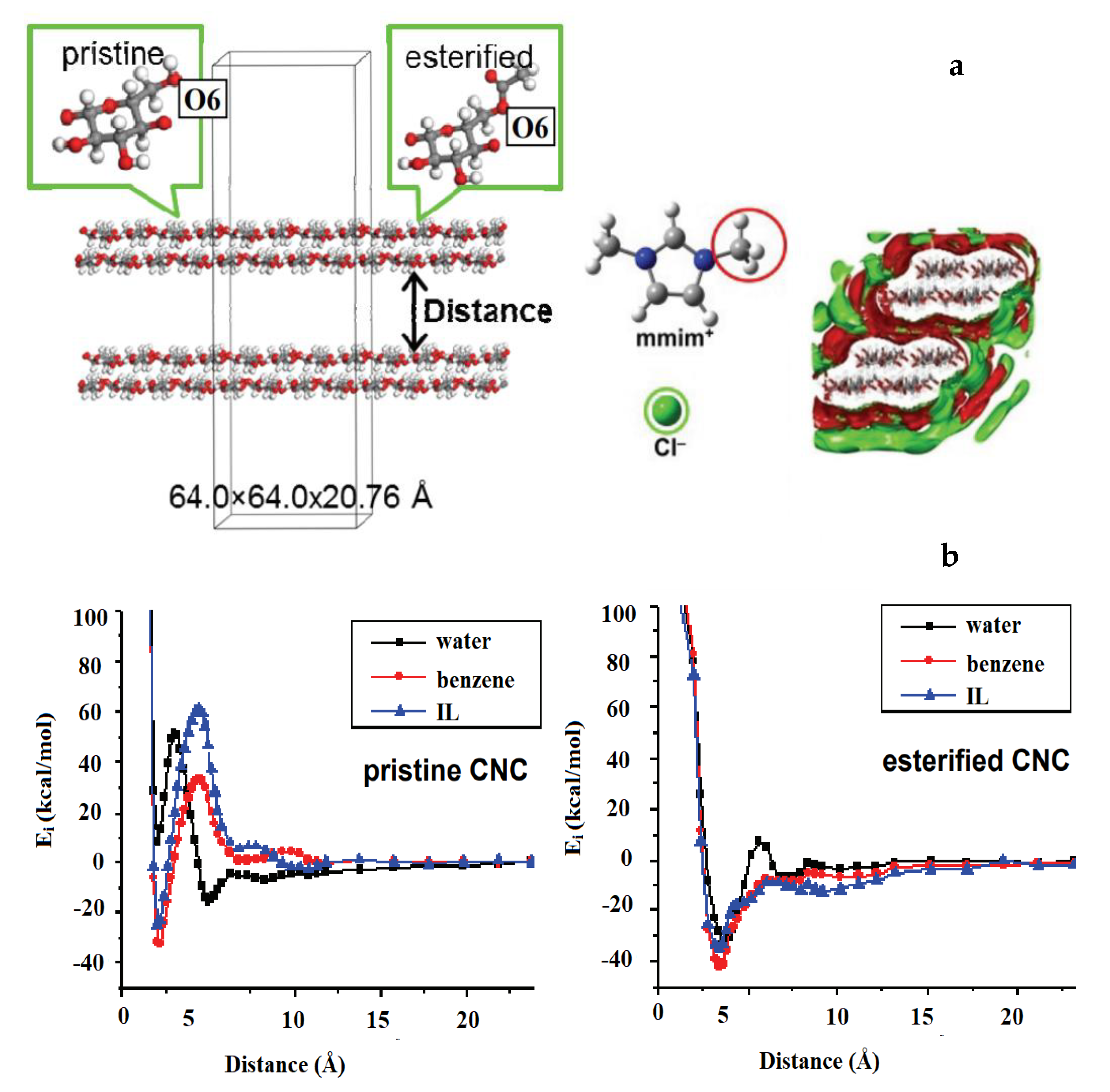
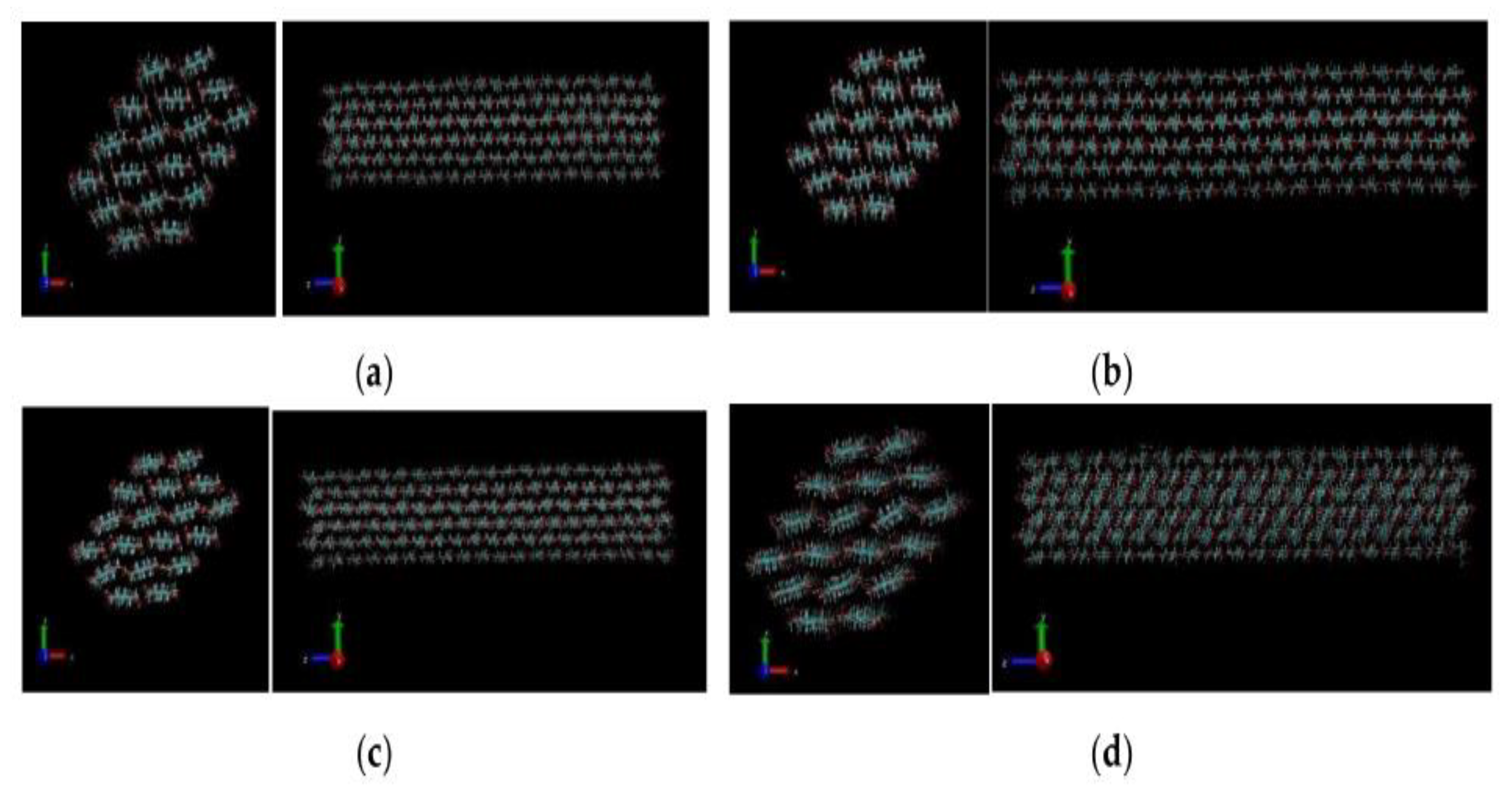
Behaviours of lignocellulosic materials when solvated or interacting with solvent molecules in addition to water were studied by Kovalenko [35]. Three-layer Iα nanocrystalline cellulose fibrils (esterified and non-esterified) of ~9 nm in length with a DP of 34 were constructed using MD. Solvation with water, benzene and ionic liquid (IL) molecules (Figure 12a) in neutral and ionic environments were studied using the 3-dimensional reference interaction site model with the Kovalenko–Hirata closure approximation (3d-RISM-KH). This method develops analytical summation of the free energy diagrams of the interaction between the macromolecule and the solvent beginning with molecular force field used. Thus, the 3D-RISM-KH integral equations for 3D site correlation functions can be obtained. Converging these site correlation functions, in turn, gives the solvation structure in terms of 3D distribution maps of solvent interaction sites around a solute macromolecule (supramolecule) of arbitrary shape. This also provides information about the solvation thermodynamics. Similar to the scale invariance of lignin structure over a limited length range. the 3d-RISM-KH method also bridges the gap between molecular structure and effective forces. However, the effectiveness of the 3d-RISM-KH is higher on multiple length scales. Specifically, in this work [35], the effective interaction (potential of mean force) plots for pristine and esterified CNC in different solvents. Similar to Iα cellulose, the Iβ cellulose is stabilized by the hydration shell. The pristine CNC disaggregation barrier increases in the order of solvents: water < benzene < IL, which indicates that dispersion is favourable in water but is not favourable in benzene and IL. This is typical for hydrophilic surfaces. For esterified CNC, the potential of mean force in benzene and IL has a lower disaggregation barrier than in water, leading to facilitated dispersion in hydrophobic solvents. The lack of significant solvent expulsion barriers in benzene and IL suggests weak solvent-solute interactions. This example demonstrates how surface modifications can be employed to tune dispersion properties of CNC in various solvents [36]. In addition to addressing the type of the surface modification, molecular simulation combined with the 3D-RISM-KH methodology allowed for the prediction of the degree of surface modification necessary to achieve a certain dispersion effect (Figure 12b).

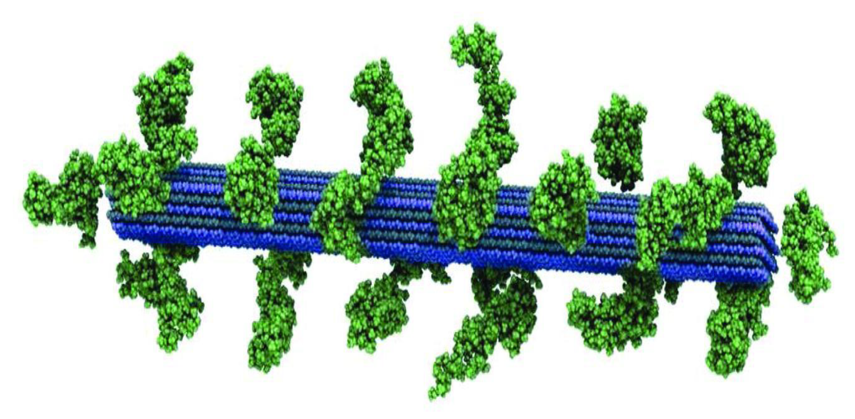
The accurate recreation of molecular mechanics is critical for the estimation of the physical properties of any simulated molecule. To this end a molecular mechanics force field was created for lignin by Petridis and Smith [23] by using the CHARMM empirical force [9] upon suitably parameterizing it. The lignocellulosic model of cellulose surrounded by lignin molecules in solution using the parameterised model in [23] built by Petridis et al. [27] is shown in Figure 13. This model was then used to probe the interactions between lignin and cellulose at the atomic level, as well as provide a way to parameterize coarse-grained mesoscale models. The constructed lignin molecules contain equal numbers of left- and right-hand linkages. The molecular weight of lignins was of the order of 10,000 or greater, and the models had a molecular weight of 13,000. Crosslinks were formed when one unit participates in more than one linkage. In total, 26 lignins were built with varying degrees of crosslinking, but the average crosslink density was chosen to be consistent with the experimental value of 0.052 obtained from spruce wood (Figure 13).

A similar parameterized CHARMM force field was applied for a multimillion atom system for lignocellulosics by Schulz et al. [37]. The main difference between the generic CHARMM force field [9] in this work and the parameterised CHARMM force field in [37] is in the expression for electrostatic potential. The general CHARMM field uses the Coulombic expression shown in Equation (20) where ε and ε₀ are the dielectric constants of the system and vacuum, q_i and q_j are the charges on atoms i and j. In [29] electrostatic potential was determined using the reaction field potential (V_rf) shown in Equation (19) where ε is the dielectric constant outside the radius rc, and r is the distance separating two charges. The reaction field potential was developed by Onsager [38] and used within the context of molecular simulation (specifically, Monte Carlo simulations by Barker and Watts [39])

$${\mathrm{V}}_{\mathrm{rf}}=\left(1+\frac{\left(\mathsf{ϵ}-1\right){\mathrm{r}}^3}{\left(2\mathsf{ϵ}+1\right){\mathrm{r}}_{\mathrm{c}}^3}\right){\mathrm{r}}^{-1}-3\frac{\mathsf{ϵ}}{{\mathrm{r}}_{\mathrm{c}}\left(2\mathsf{ϵ}+1\right)}$$

(19)

$${\mathrm{V}}_{\mathrm{C}}= \frac{1}{4{\mathsf{\pi }\mathsf{\epsilon }\mathsf{\epsilon }}_0}\frac{{\mathrm{q}}_{\mathrm{i}}{\mathrm{q}}_{\mathrm{j}}}{{\mathrm{r}}_{\mathrm{ij}}}$$

(20)

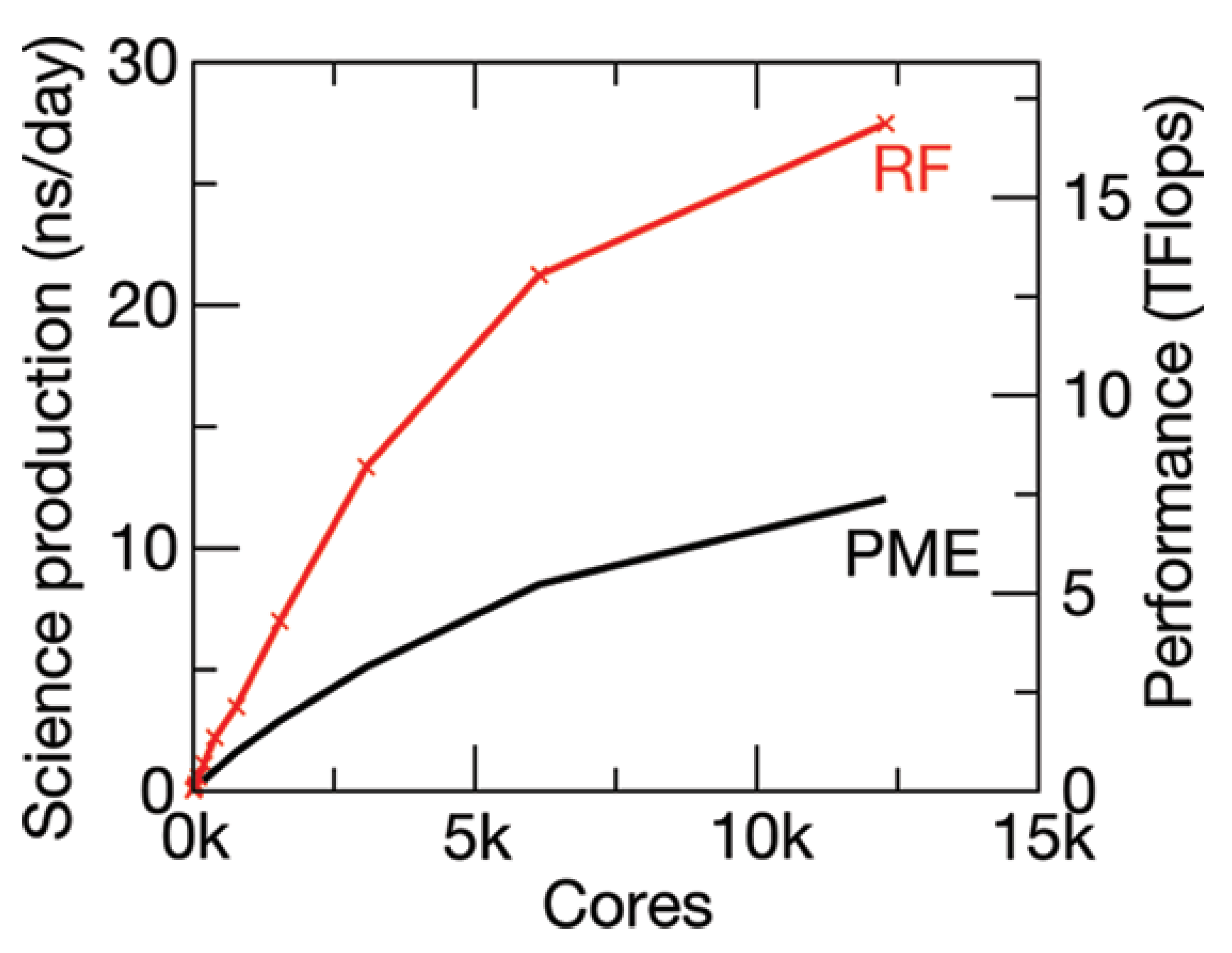
Using Equation (19), Schulz et al. [37] were able to demonstrate the scalability and efficiency of their reaction field method over the conventional particle mesh Ewald summation method. Up to three million- and five million atom simulated systems were studied and ∼30 ns/day was achieved. This represents a massive improvement on existing MD methodologies. The scalability differences between the PME and the RF method [38] can be clearly seen in Figure 14.

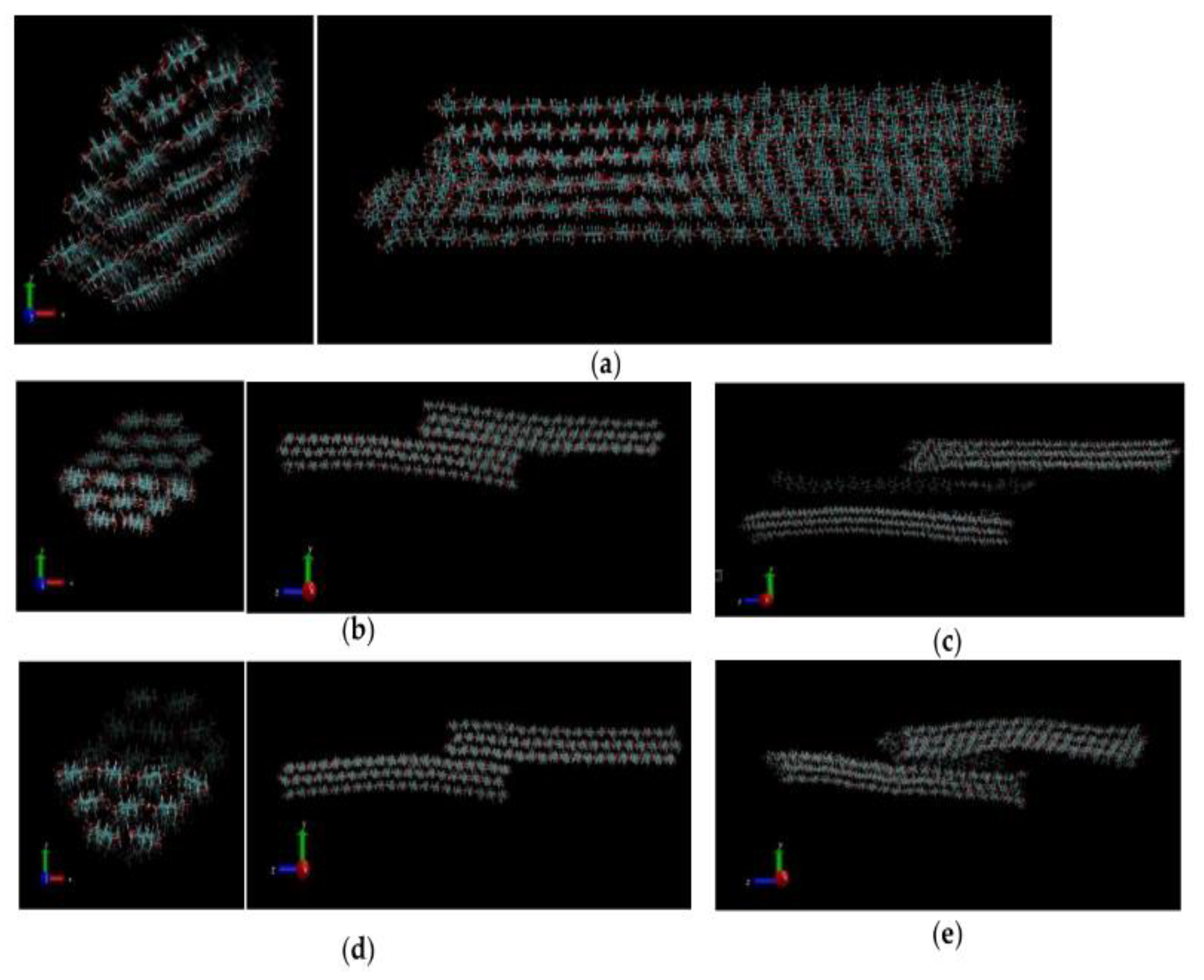
The proof of concept established by Schulz et al. in [37] showed the viability of simulation of multi-million atom lignocellulosic systems by using the reaction field method. Building on that Lindner et al. [40], built 3.31, 3.43, and 3.80 million atom lignocellulosic systems and ran the simulations on the Jaguar XT5 Petaflop Supercomputer using 40,000 cores at a peak performance of 27 ns/day similar to the work of Schulz et al. [37]. The work of Lindner et al. 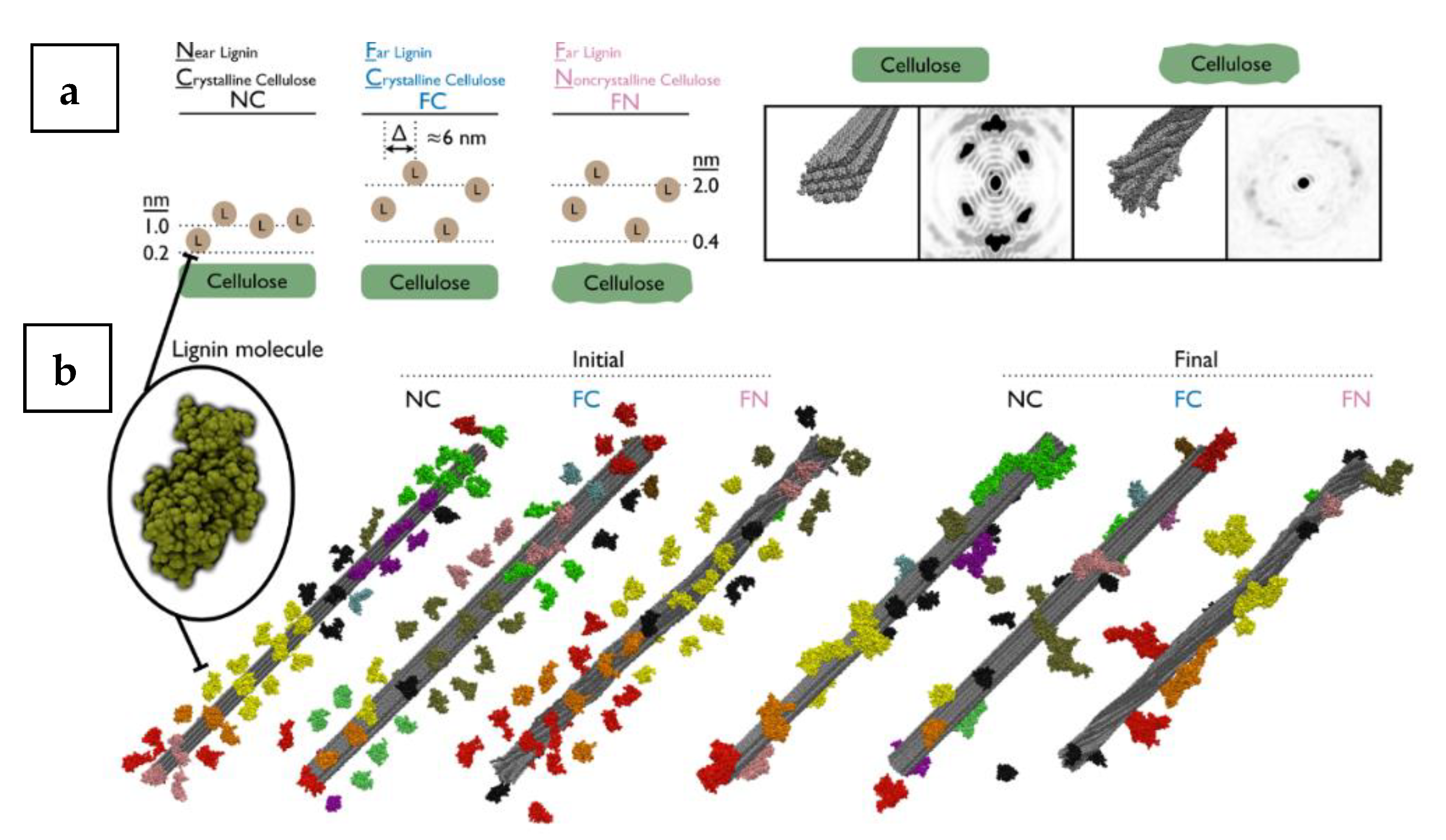[40] is one of the largest-ever atomistic biomolecular MD simulations conducted to date. The lignin molecule modelled consists of 61 monomers, corresponding to a molecular weight of 13 kDa while the cellulose fibre model consisted of 36 chains with a chain length of 160 monomers (Figure 15). The lignins were simulated with crystalline (FC, FN) and non-crystalline cellulose (NC) models. For each model, 52 lignin molecules were placed around the central cellulose fibre (at distances randomly chosen within the interval of 0.2 to 1.0 nm and 0.4 to 2.0 nm) for the NC model, the FC (crystalline cellulose with initial lignin position far from the central fibre) and FN (crystalline cellulose with initial lignin position far from the central fibre) models, respectively. The simulations were performed with the GROMACS [11] suite using the TIP3P water model and the CHARMM Carbohydrate Solution Force Field (CSFF) for cellulose and the CHARMM Lignin Force Field similar to previous works on lignocellulosics [21,34,37]. The MD simulation was able to produce simulated directional X-ray scattering peaks diagram along the fibre axis. This is shown for both the crystalline and the non-crystalline cellulose, (Figure 15a). It was found that the models with the crystalline cellulose exhibited strong Bragg peaks, which were absent in the non-crystalline model.

The results of Lindner et al. [40] shone a light on the intrinsic processes that determine the nature of lignin precipitation onto cellulose and the dependence on cellulose crystallinity thereof. Their results showed that lignin has a strong tendency toward aggregation with lignin and cellulose. The simulations also revealed that the average direct interaction energy between lignin and cellulose is independent of cellulose crystallinity. However, lignin aggregation onto non-crystalline cellulose was found to be less favourable than for the crystalline form, owing to the significantly different solvation properties of crystalline and amorphous cellulose.

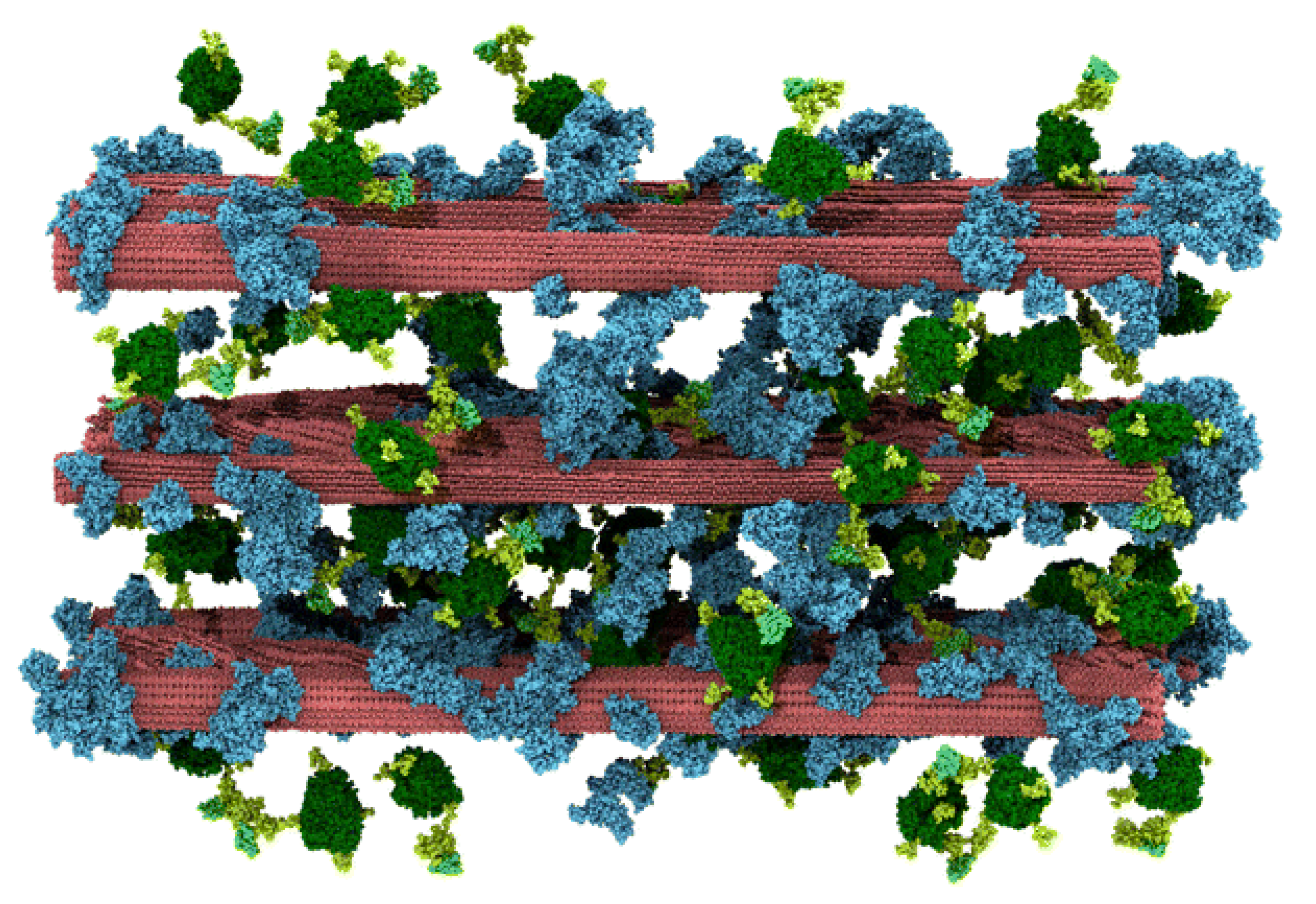
Biomass is also converted into functional products using enzymatic methods, specifically hydrolysis. This process is also inhibited by the presence of lignin similar to [40]. To this end, Vermass et al. [41] used MD for elucidating the atomistic/molecular aspects of lignin inhibition of enzymatic hydrolysis. The RFZ equation was used for electrostatic interactions similar to Schulz et al. [37]. The constructed model shown in Figure 16 represents the largest biomass MD simulation at 23.7-million atom. The total simulation time was 1312 ns. The simulations were carried out on the TITAN XC6 Supercomputer at Oak Ridge National Laboratory, using 60,000 cores at a peak performance of 45 ns/day higher than the 27 ns/day achieved in [37] and [40]. The multi-component simulation model was built to represent a pre-treated biomass system of cellulose and lignin at room temperature upon the addition of cellulolytic enzyme and is shown in Figure 16. The model consists of cellulose fibres, lignin molecules, and Cel7A cellulases. Other components of biomass, such as pectins and hemicellulose, were assumed to have been removed by dilute acid pre-treatment.

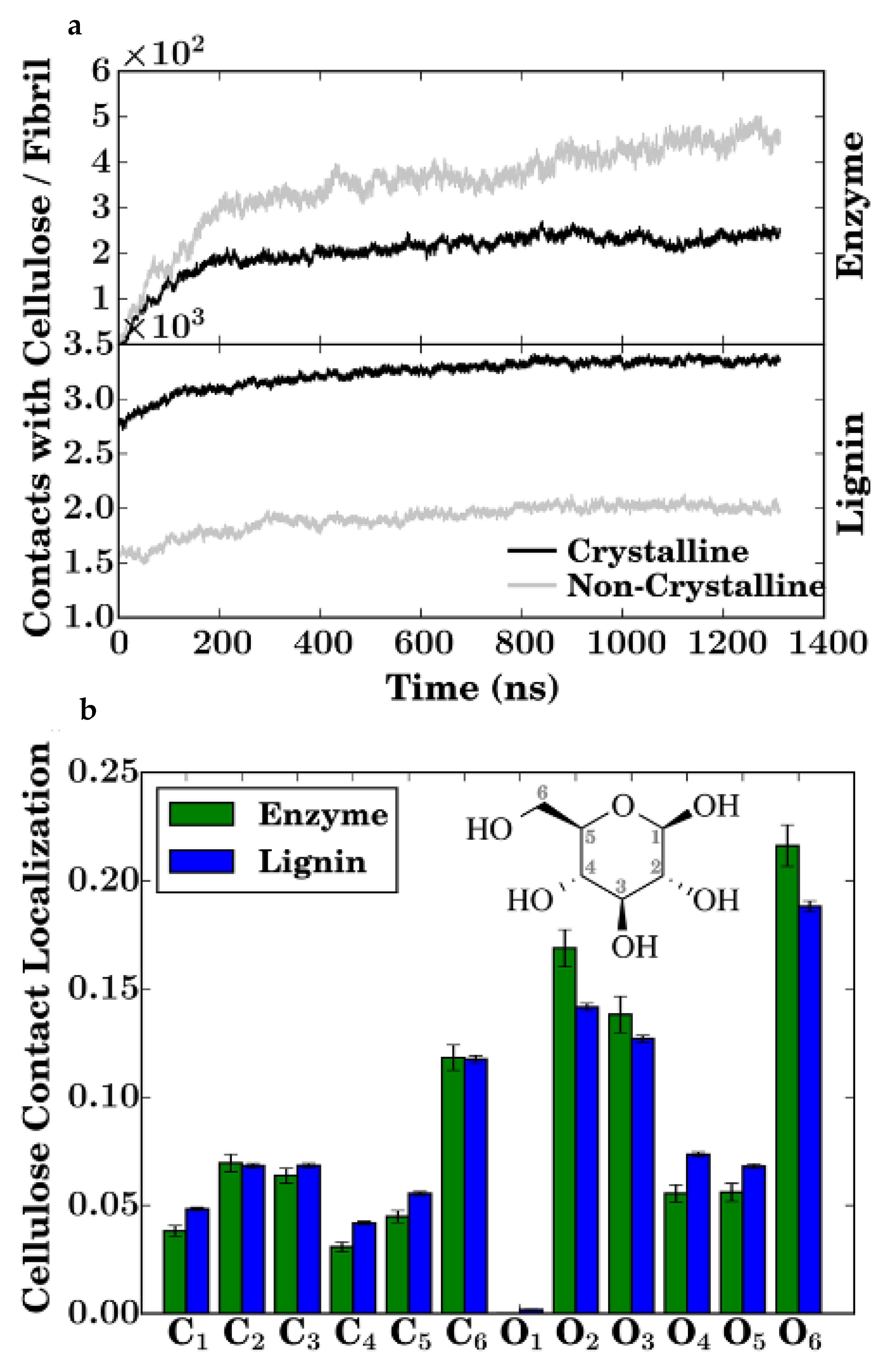
In the initial parts of the simulation, the lignin-lignin and lignin-cellulose interactions did not change significantly. As the simulation progresses a gradual increase in the number of enzymatic contacts to the lignin and cellulose phases were observed as the enzymes diffused to the lignocellulose. It was observed that the lignin mediates the formation of a fully interconnected network of cellulose, lignin, and enzyme, with each molecule linked to all others directly or indirectly. The enzymatic diffusion was also mediated by the lignin. The binding of the enzyme to cellulose or lignin led to a three orders magnitude reduction in the translational diffusion coefficient of the enzyme (∼10⁻⁶ cm²/s initially to ∼10⁻⁹ cm²/s at the end of the simulation). After equilibration, the surfaces of the cellulose fibrils in the simulated model were analysed. Similar to the process of cellulose precipitation investigated by Linder et al. [40], the enzymatic destruction of lignocellulosic biomass is also inherently dependent on the binding of the enzyme (in [41], being TrCel7A cellulase) to the cellulose. There exists a close interaction between lignin and the enzyme. 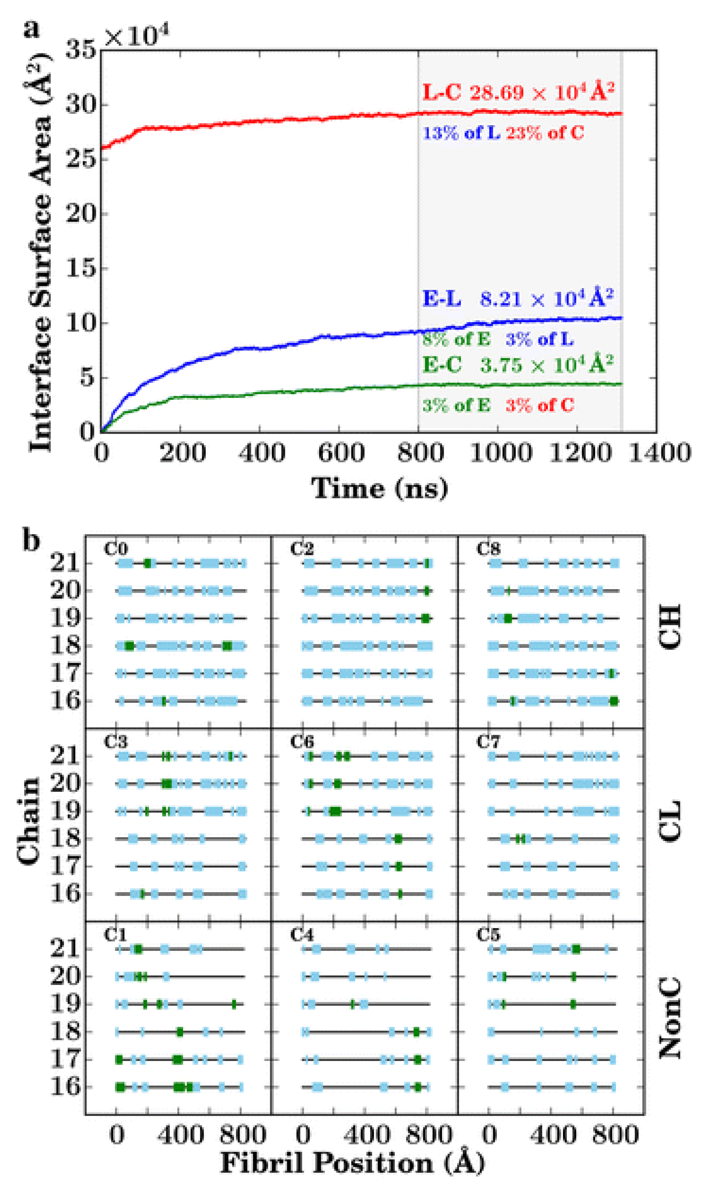This, in addition with the mediation of the enzyme diffusion by the lignin results in the lignin outcompeting the cellulose in terms of binding to the cellulose-binding module (CBM) of the enzyme (Figure 17a,b). From the simulation it could be observed that the flat hydrophobic surface on the CBM (formed by three tyrosine residues) which should promote binding to the hydrophobic surfaces of the cellulose fibres instead forms extensive contacts with the lignin. The cellulose surface, also, is crowded by the lignin with nearly 25% of the total cellulose surface area being consistently covered by lignin, significantly reducing the area accessible to the enzymes (Figure 18a,b). Therefore, the presence of lignin molecules on the cellulose surface interferes with the mechanism of cellulose hydrolysis. The lignin molecules adhere to the surface of the cellulose fibres, slow the diffusion of the enzymes and out-compete the cellulose for contact with the enzyme CDM and thus, reduce the distance an enzyme bound to cellulose can travel before its path is blocked by a lignin molecule. Large scale simulations such as this one carried out by Vermass et al. [41] and Lindner et al. [40] provide a visual and graphical view of the fine molecular interactions that, in turn, affect industrial process such as enzymatic hydrolysis.

Therefore, over the past quarter of a century, the simulation and modelling of lignocellulosic systems has come a long way. Lignocellulosic systems ranging from a few hundred to several million molecules have been constructed, simulated, validated through molecular characterization. Fine structural characteristics of these systems that control the physical and biochemical properties of the lignocellulosic systems in the presence of water and other solvents, ions and enzymes have been unearthed through a combination of MD with mathematical and visual methods. The next step is to use these validated simulations to predict mechanical behaviour of the lignocellulosic phases namely, lignin and cellulose and the lignocellulosic composites which is covered in the next section.

2.2. Mechanical Behavior Prediction of Lignocelluloics Using MD

2.2.1. Cellulosics

Cellulose fibres isolated from lignocellulosics consist of crystalline regions and amorphous regions. The elastic modulus of the crystalline regions of cellulose is quite important while aiming for its use in composites and structural applications [42]. Muthoka et al. [42] reported on the history of theoretical attempts of predicting the moduli of the different polymorphs of crystalline cellulose and noted the use of X-ray diffraction, Raman spectroscopy and Atomic Force Microscopy (AFM) for this purpose [34]. Cellulose exists in various crystalline polymorphs viz., Iα, Iβ and II and so, the first MD attempt for cellulose Young’s modulus estimation was done in 1996 [43] for cellulose Iα. In this first attempt, the simulated Young’s modulus for cellulose I was found to be 134–135 GPa [43]. Attempts on the MD based modelling of regenerated cellulose fibres was done in [22] and at room temperature, the longitudinal modulus of regenerated cellulose was found to be 155 GPa. The novelty of that work was based on the unconventional use of the constant particle number (N), constant external stress tensor (p or t) and constant enthalpy H (NpH or HtN) ensemble for the MD simulation. Elastic modulus estimation of crystalline cellulose was estimated using the COMPASS program and the PCFF force field in [44] and the reported Young’s modulus values ranged from 124 to 155 GPa. The so-called second-generation force fields were found to be superior to the first-generation ones (specifically, CVFF used in [21]) for the optimization of cellulose structure. Eichorn and Davis [45] conducted a holistic analysis of cellulose mechanical properties. Both the compressive and tensile deformation of various models of structures of crystalline regions of all cellulose polymorphs were studied by MD techniques using the proprietary COMPASS force field as in [44]. The models for cellulose Iα, Iβ and II constructed in [45] are shown in Figure 19. In order to obtain a simulated modulus value (referred to in [45] as the chain modulus), the simulation box containing the cellulose model of appropriate crystal phase was repeatedly strained and its energy minimised with respect to the atomic positions. This was done whilst maintaining the deformed cell shape, to yield the energy as a function of imposed strain. This allowed for the determination of all the elements of the compliance matrix S. S could then be inverted and the chain modulus could be calculated from the inverse of the appropriate matrix component. To ensure the appropriate starting energy, the energy of the undeformed structure, which is obtained by full minimisation of the structure with respect to atomic coordinates and lattice parameters, was needed. the minimization was performed in two steps; in the first step the atomic co-ordinates were varied using constant cell parameters and in the second step both the atomic co-ordinates and the cell parameters were allowed to vary. For cellulose Iα the modulus value obtained from analysing Figure 19a was 155 GPa while that from analysing Figure 19d was 136 GPa. For cellulose Iβ, the modulus value from analysing Figure 19b was 116 GPa while that from analysing Figure 19e was 149 GPa and finally for Cellulose II, the modulus value from analysing Figure 19c was 166 GPa while that from analysing Figure 19f was for 109 GPa.

Wu et al. [46] confirmed the anisotropy of cellulose tensile behaviour using MD. A model of Iβ cellulose was deformed in the three orthogonal directions (corresponding to the a, b, and c parameters of the cellulose unit cell) at three different strain rates. The stress–strain behaviours for each case were analysed and then used to calculate mechanical properties (including the elastic modulus value). The results showed that the elastic modulus, Poisson’s ratio, yield stress and strain, and ultimate stress and strain were highly anisotropic, thereby confirming real material behaviour. In Wu et al. [46], the cellulose unit cell was constructed using the following lattice constants- a = 0.7784 nm, b = 0.8201 nm, c = 1.0380 nm. This unit cell was then expanded 4 × 4 × 8 times in the three orthogonal directions to obtain the simulation system. The constructed simulation system was relatively small (~ 5 nm in the transverse directions and ~10 nm in the chain direction) and is shown in Figure 20.

The main difference between the work of Wu et al. [46] and the other works referenced in this review is the use of the ReaxFF reactive type force field for carrying out the MD simulation. All other works have used parameterized but non-reactive force fields (such as CHARMM, DREIDING, PCFF, etc). Using the ReaxFF force field, Wu et al. [46] claim to capture the breaking (and potentially formation) of covalent bonds due to strain. To apply strain, the simulation system was deformed in the three orthogonal directions with the deformation in each direction being performed independently. Tensile strain was applied in each direction by elongating the simulation cell by a small increment (about 0.25 %). The system was then re-equilibrated in the NPT ensemble at 1 atm of pressure applied in the two non-deformed directions in order to allow their dimensions to change. The system was strained and equilibrated repeatedly until 100 % strain was reached. By modelling large strain, i.e., beyond the initial elastic and plastic deformation, Wu et al. [46] were able to obtain the full strain response of the material and propose failure mechanisms. The strain rate of the tensile deformation was controlled by changing the equilibration time from 0.25 to 2500 ps to achieve strain rates from 10⁻² to 10⁻⁶/ps although no data for the 10⁻⁶/ps system was reported. It has to be noted that all the acquired data are values averaged over the last 10 % of simulation time at each equilibration step similar to the work in [33]. The results of Wu et al. [46] are detailed in

Table 3. Mechanical data for Cellulose Iβ using MD in all orthogonal directions. With permission from [46].

Strain Rate	10−4/ps			10−3/ps			10−2/ps
Deformation Direction	X	Y	Z	X	Y	Z	X	Y	Z
Elastic Modulus (GPa)	21.6	7.6	107.8	22.7	7.1	113.5	24.4	6.5	112.9
Yield Stress (GPa)	0.3	0.2	4.6	0.4	0.3	5.4	0.6	0.4	6.6
Yield Strain (%)	1.3	2.3	4.3	1.8	4.1	4.9	2.5	5.9	5.9
Ultimate Stress (GPa)	0.4	0.3	5.4	0.7	0.4	6.0	0.9	0.5	7.2
Ultimate Strain (%)	3.0	7.5	5.1	4.6	9.4	5.4	6.2	11.3	6.7

. Based on the simulated data, Wu et al. [38] were able to make the following observation. First, that the axial modulus values (107.8 GPa–113.5 GPa) were comparable to experimental values (105 GPa–220 GPa). Second, that the transverse moduli (21.6 GPa–24.4 GPa in x direction, 6.5 GPa–7.6 GPa in y direction) were also comparable to experimental data (2 GPa–50 GPa). Third, H- bonding dominates the response of the crystal to strain in the x-direction and H- bonds are very short-range i.e., at small strain the H- bonds are very strong but the strength of those bonds falls off quickly with increasing strain, resulting in the strain at yield in the x-direction being the smallest of the three directions. Fourth, that the ultimate stresses are comparable while the ultimate strain in the y-direction is larger than that in the x-direction. Like the yield behaviour, this was attributed to the strong, yet short ranged nature of the H-bonds resisting tension in the x-direction. Finally, for both the single chain and the cellulose Iß, the covalent bonds within the chains are strong, resulting in very large ultimate strength.

Tensile behaviour of nanocrystalline cellulose was also estimated by Muthoka et al. [42] using MD. They developed a novel steered pull MD technique wherein while applying an external force to a group of atoms, one could opt to keep other groups of atoms fixed, where various behaviours of interest could then be investigated. In this pull simulation case, Muthoka et al. [42] took into account cellulose nanofiber structure in order to investigate the mechanisms beyond its mechanical properties. By analysing the secondary molecular interactions and the H-bond network formation a better insight on molecular structure and behaviour could be obtained. This could then be exploited to enhance compatibility of nanocrystalline cellulose with other polymers to produce high performance materials with predictable tensile behaviour and moduli. The cellulose model used in [42] was a cellulose Iβ based on X-ray diffraction measurements and unit cell specification as done in [47]. A hexagonal nanocrystalline cellulose model was made with 36 chains with each chain consisting of 20 glucose residues. The force field used was an all-atom optimized potential for liquid simulations (OPLS-AA), a force field extended for carbohydrate simulations. The simulation temperature was set at 300 K. The system consisted of 7614 cellulose model atoms, 333,564 water molecules, 210 chlorine ions, and 210 sodium ions. Prior to the actual MD simulations, energy minimization and equilibration steps were carried out. Equilibrations were carried out in the NVT and NPT ensembles at 300 K. The steered pull MD runs were carried out for 200 ps also at 300 K at different pulling rates under conditions defined by case 1 (shown in Figure 21) and case 2 (shown in Figure 22).

The effect of simulated pulling on the structures under testing conditions in case 1 and case 2 are shown in Figure 23 and Figure 24 respectively. As the pulling force increases, a structure with revealing disruption in bonding is observed. This phenomenon can be ascribed to the opening up of hydrogen bonding network. Under applied force, the hydrogen bonds in the cellulose model are susceptible to disruption as stretching of the bonds leaves the chains vulnerable to possible sliding with respect to one another. In Figure 23, at low pulling force (1000 kJ/mol/nm), the disruption of the molecular structure of the atoms in the cellulose model is minimal and observed to increase as the pulling force increases with an extreme disruption depicted at 50,000 kJ/mol/nm.

In Case 2, at a low pulling force (5000 kJ/mol/nm), the cellulose model chains were observed to slowly separate along the interface of the fixed chains and the chains subjected to the pulling force. Additionally, there was no observed separation of the chains for the greater part of the simulation time. However, towards the end of the simulation time, the chains were observed to separate slowly to the extent presented in Figure 24a. The sliding mechanism of cellulose nanofibers can be attributed to successive sliding of cellulose atoms on top of each other. At 10,000 kJ/mol/nm and 50,000 kJ/mol/nm, separation was observed within the first few picoseconds of the MD simulation. Complete separation was observed at the end of the simulation at these higher pull forces. In addition, it was noted that complete separation at 50,000 kJ/mol/nm in Figure 24d,e was attained faster (within few picoseconds of simulation) than that observed at 10,000 kJ/mol/nm in Figure 24b,c.

The results of case 1 were used to build up the stress strain relationship of the simulated cellulose molecules and is shown in Figure 25. The strain values were determined by the ratio of elongation (difference of initial length from the final length) to the initial length of the non-frozen atoms where the pull force was applied. To obtain the corresponding stress to the applied force, the pull force, kJ/mol/nm was converted into Newton by relation to the Avogadro’s constant per mole and then dividing it by the cross-sectional area of the cellulose fibres simulation structure. The stress–strain relationship deduced a Young’s modulus of 161 GPa for all the 18 chains of cellulose fibres. This value of modulus obtained using the modified AA-OPLS force field for carbohydrates was a bit higher as compared to the previously achieved values using previously simulated values as in [46].

The average chain length of the cellulose nanocrystals found in real life wood samples are of the order 100–200 nm and to this end, a supra coarse-grained MD approach for estimating cellulose mechanical properties was developed by Mehandzhiyski et al. [48]. This coarse-grained approach was based on atomistic molecular dynamics simulations and was developed with the force matching coarse-graining procedure. Coarse-grained approaches are able to significantly reduce the degrees of freedom in molecular simulations and therefore to explore larger systems at a much longer time scale compared to regular atomistic MD. Through this approach, Mehandzhiyski et al. [48] were able to parameterize an OPLS-AA force field for coarse grained approaches, demonstrate the self-assembly of the cellulose nanocrystal chains and validate the developed model. The validation of the coarse-grained model developed in [48] was done through comparison with experimental and simulation results of the elastic modulus, self-diffusion coefficients and cellulose fibre twisting angle. Similar to [42], the coarse grained model in [48] initially consisted of 36 chains of cellulose Iβ arranged in hexagonal shape. The 36 chain model had dimensions of 3 × 5 nm similar to a wood derived CNC, which has a typical width of 3–5 nm [49]. The model of Mehandzhiyski et al. [48] is shown in Figure 26. All simulations were carried out with the GROMACS [11] simulation package, in an implicit solvent. The van der Waals cut-off and the neighbour list were set to 32 Å- a much higher value as compared to the other works referenced in this review (these tend to be from 8 to 12 Å). The simulation snapshots were prepared with VMD and pymol. The force field parameterization in [48] followed the least squares fitting method to minimize the objective function as shown in Equation (21). $F_{il}^{Ref}$and $F_{il}^p$ are the reference and predicted force acting on the i^th atom in the l^th configuration, respectively, and depends on the set of M parameters; N is the number of atoms in the atomistic MD configuration and L = 5000 is the total number of atomic configurations used in the fit.

$${\mathsf{\chi }}^2=\frac{1}{3\mathrm{LN}}{\displaystyle \sum }_{\mathrm{i}=1}^{\mathrm{L}}{\displaystyle \sum }_{\mathrm{i}=1}^{\mathrm{N}}{\left|{\mathrm{F}}_{\mathrm{il}}^{\mathrm{Ref}}-{\mathrm{F}}_{\mathrm{il}}^{\mathrm{p}}\left({\mathrm{g}}_{\mathrm{i}},\dots .,{ \mathrm{g}}_{\mathrm{m}}\right)\right|}^2$$

(21)

The translational diffusion coefficients were presented as a function of the cellulose nanocrystal chain length which was varied between 50 and 1200 nm. In total, 20 cellulose nanocrystal chains were placed randomly in a simulation box where the initial separation distance between the cellulose nanocrystal chains was at least 100 nm to ensure no initial interactions between the chains. The simulations were run for 1000 ns each and the diffusion coefficients D is calculated in a standard way from the mean-square displacement using the Einstein relation, as in [32,33] amongst others. The calculated diffusion coefficients of the cellulose nanocrystals showed an exponential decay with the increase of the length. They varied between 17 and ~1 × 10⁻¹² m²/s for lengths between 50 and 1200 nm, respectively. These were compared with experimental values found in [50,51,52,53] and an excellent agreement was found (Figure 27a). This way to validate polymer models using diffusion coefficients was also used for semi-crystalline polyethylene by Prasad et al. [32]. Axial modulus of a single coarse grained cellulose fibril was obtained by pulling one end of the coarse-grained model while keeping the other end fixed. A modulus value of 110 GPa (Figure 27b) was obtained which is similar to the values obtained in [43,44,45,46]. Mehandzhiyski et al. [48] went one step further and studied the self-assembly of the cellulose nanocrystal chains. They allowed the simulation to proceed from initial condition (corresponding to a cellulose volume fraction of 1% in the simulation box) to about 15,000 ns (corresponding to a cellulose volume fraction of 4.5% in the simulation box) at a pressure of 2 bar and 300 K temperature, thus simulating evaporation of the implicit solvent. The evolution of the volume fraction is shown in Figure 27c. The system obtained from the evaporation simulation (d) was subjected to a constant rate of deformation at two different rates, 2 × 10⁻⁴ nm/ps and 1 × 10⁻³ nm/ps. In the direction of the applied strain the compressibility of the box was set to zero (incompressible) and in the transverse directions was set to 4.5 × 10⁻⁵ bar⁻¹ and the pressure to P = 1 bar. The effect of the deformation on the simulation box is shown in Figure 27e. The modulus thus estimated is essentially the elastic modulus of a cellulose hydrogel. Modulus values of 7.2 MPa and 12.7 MPa were obtained for the deformations rates of 2 × 10⁻⁴ nm/ps and 1 × 10⁻³ nm/ps, respectively, which were in the range of the reported elastic modulus of cellulose hydrogels, 1–50 MPa [54,55,56,57].

The mechanical properties of cellulose with structural deformities were studied using MD by Khodayari et al. [58]. They noted that deformities (termed as dislocations) not only exist in microfibril scale (elementary fibres), but also within the cellulose nanocrystal units, connecting the crystalline regions together in series. Therefore, in [58], the mechanical properties of cellulose nanocrystal chains in the presence and absence of these dislocations was determined. Additionally, the effect of hydrogen bonding on the longitudinal tensile modulus of the fibrils is assessed. It was also shown how water can alter the surface characteristics of the cellulose nanocrystal chains, leading to changes in elastic properties and a mechanism for re-crystallization of the disordered regions within the cellulose nanocrystal units was investigated. MD was carried out using the 2018 version of GROMACS [11] suite. The GLYCAM06 force field obtained by parameterization of the AMBER [10] force field was used for carrying out the MD simulation. The steepest decent minimization algorithm is used to minimize the energy of the systems. A leap-frog algorithm was used to integrate the Newton’s equations of motion for the NVT, NPT, and production run. Constraints were applied on the bonded hydrogens through the Linear Constraint Solver (LINCS) algorithm similar to [34]. Neighbour searching was performed by the Verlet scheme, having a cut-off for short-range electrostatics and van der Waals interactions of 1.2 nm, using grid cell neighbour searching. Electrostatics were treated by the particle- mesh Ewald (PME) method. Temperature coupling is performed by a velocity rescaling thermostat, with a time constant of 0.1. Pressure couplings was applied using a Parrinello–Rahman barostat, creating isotropic pressure on the system, with a time constant of 0.1, keeping the pressure at 1 bar with a compressibility of 4.5 × 10⁻⁵ for the hydrated models. Periodic boundary conditions were applied in all directions, when water was present. A 6 × 6 Iβ crystalline cellulose model, DP 30, was built in the MATERIALS STUDIO program in a 10 × 10 × 25 nm³ simulation box. The energy minimization step was followed by a 1 ns NVT ensemble simulation and a 2 ns production run. Temperature was kept constant at 300 K under implied vacuum and in the presence of water. A schematic of the cellulose monomer unit is shown in Figure 28.

A model consisting of two crystalline sites, connected through a dislocated region in the middle was constructed to represent a dislocated cellulose chain (Figure 29). The dislocated section consisted of 10 glucose units and built through three tempering MD cycles- 1 ns at 750 K, 1 ns at 900 K, and 1 ns at 1100 K. At each step, the temperature was increased gradually so that the structure does not explode due to high kinetic energy exerted. Following these cycles, a quenching cycle for 1 ns at 300 K was performed to stabilize the model.

The elastic modulus of the models was computed by applying a constant deformation on the glucose units at the two ends of the fibrils, providing a strain rate of 0.08 ns⁻¹. The Young’s modulus for purely crystalline model of cellulose was calculated to be 146.6 ± 0.7 GPa, whereas this value dropped to 109.3 ± 0.6 GPa for the dislocated model (Figure 30). To further investigate these models, Young’s modulus of a fully dislocated model was calculated and turned out to be 80.5 ± 0.9 GPa. It was also estimated that the dislocated region showed a strain almost 1.8 times the crystalline regions. Another interesting observation was that the modulus of the dislocated cellulose could be modelled using the rule of laminates (also used extensively for transport property modelling [32,33]). Therefore, the elastic modulus of the fibrils and crystalline cellulose could be then used to measure the amount of dislocated cellulose in any given sample.

Based on the existing research, mechanical properties of cellulose have been explored extensively using MD. Size ranges of the simulated systems range from single crystals (Iα, Iβ and II polymorphs) [31,43,44,45,46], atomistic [43,46,48] and coarse-grained [58] models. MD suites such as GROMACS [48,58], VMD [48] and MATERIALS STUDIO [44,45] have been used for this purpose with force fields such as PCFF [44], COMPASS [44,45], ReaxFF [46], AMBER/GLYCAM [58] and OPLS-AA [42,46,48,58]. MD ensembles used were NVT [42,58] and NPT [42,46,58] and mathematical treatments such as force field parameterization [48,58] and compliance matrix estimation [45] were used. The mechanical properties that have been investigated include the moduli of single crystals [42,44,45,46], moduli in all orthogonal directions [46] and tensile, shear and yield behaviour by using steered pull techniques [42]. Therefore, a holistic view of cellulosics has been achieved through MD simulation.

The use of MD for the mechanical characterization of lignins is now investigated in Section 2.2.2.

2.2.2. Lignins

From Section 2.1, the use of MD for the validation of lignin and lignin-based compounds is quite established [23,27,34,37]. Lignin from wood has the potential to be the main natural source of aromatic compounds which, in turn, could be essential raw materials for use in the renewable carbon materials, plastics, resins, composites, additives, foams, surfactants, and membranes industry [59]. However, as compared to cellulosics, progress on the extraction/modification/application of lignin is quite low owing to its recalcitrance and complexity [59]. A MD analysis of this recalcitrance was done in [37,40,41] and a molecular mechanism for the inhibitory effects of lignin on the cellulosic phase of lignocellulosics was established. In addition, hydrogen bonding, intramolecular interactions, conformations in water and solvent, interactions with enzymes and thermal properties of lignin have also been simulated [20,21,27,34,37,40,41].

The first attempt at measuring the mechanical properties of Periodate and Klason extracted lignin in dry and wet conditions were conducted by Cousins [60]. They found that the as moisture content was increased from 3.6 to 12% the Young’s modulus of periodate lignin decreased linearly from 6.7 to 3.1 GPa and the shear modulus from 2.1 to 1.2 GPa. From moisture content 0 to 3.6% there are small but poorly defined increases in moduli. Klason lignin modulus values were usually much lower than the corresponding moduli for periodate lignin and the initial increase from 0 to 3% moisture content did not occur. From 3 to 12% the Young’s modulus fell from 4 to 2.3 GPa, and the shear modulus from 1.5 to 1.1 GPa [60].

A MD validation of the effect of moisture on lignocellulosics was done by Youssefian et al. [61,62]. In this section, we will concentrate on the lignin results and the results of the simulation of the lignin-carbohydrate complex and overall wood properties will be covered in Section 2.2.3. The structural model of lignin used in [61] consisted of 28 subunits of lignin proposed by Sakakibara [63]. In this model, the value of the structural units and the number of protons per C9 structural units were chosen as to be close to that of spruce milled wood lignin. The effects of moisture uptake on the simulated lignin on the density and elastic modulus was determined in [61] (Figure 31) and is compared and contrasted with hemicellulose and the so-called lignin carbohydrate complex (LCC), which will be covered in further detail in Section 2.2.3. It can be seen introducing a small amount of water (less than 2.5%) into dry LCC and lignin does not change their densities significantly whereas hemicellulose density decreases notably. As the water molecules continue permeating into these polymers, their densities decrease almost linearly. The elastic modulus of hemicellulose drops almost linearly with increasing water content whereas lignin and LCC elastic moduli increase at low water content (less than 10%) and decreases afterwards. The peaks in elastic moduli are at 2.5% and 10% MC for LCC and lignin, respectively. The effect of the water molecules are as follows: when water molecules initially permeate into the polymer, they enhance the elastic modulus of the material. This is because at low moisture contents, hydrogen bonds between the lignocellulosic chains and water molecules seem to be more favourable than water-water hydrogen bonding. Once the number of water molecules inside the material reaches a certain level, the effect of water molecules becomes regressive and the modulus of elasticity starts to decrease. at low moisture contents. Essentially, at higher moisture contents, the water molecules tend to make hydrogen bond with other water molecules and form nano-droplets inside the lignocellulosic materials.

Another attempt at simulating the thermomechanical properties of lignin was conducted in [62]. In total, 8 lignin molecules based on the structure in [64] were utilise and to estimate the Young’s modulus, the periodic structures were expanded along each direction to the maximum strain amplitude of 0.01 in 10 steps. It can be seen from

Table 4. MD simulated vs. experimental properties of lignin. With permission from [62].

System	Simulated Density (g/cm3)	Experimental Density (g/cm3)	Simulated Glass Transition Temperature- Tg (°C)	Experimental Glass Transition Temperature- Tg (°C)	Simulated Young’s Modulus (GPa)	Experimental Young’s Modulus through Nanoindentation (GPa)
Lignin	1.26 ± 0.02	1.33	140.26	97–171	5.90 ± 0.37	2–6.7

that the lignin model estimates the real densities within 5.2%. It is known that the Young’s modulus of a material is defined by its resistance to the tension or compression of atoms and molecules and is affected by factors such as interatomic and intermolecular energies per unit volume. However, for amorphous materials such as lignin, the applied stresses are mostly used to overcome the non-bonded energies between the molecules because they unwind the chains rather than directly struggle with the energies of bonds between the atoms. Therefore, at small strains, non-bonded energies were found play more important roles in determining the elastic moduli of amorphous materials and such observations could only be made under MD treatment.

The effects of moisture and temperature on lignin mechanical properties was demonstrated by Zhang et al. [65] using MD and grand canonical Monte Carlo (GCMC) simulations. Using the structure shown in Figure 32a, Zhang et al. [65] built a model of softwood lignin consisting of 9000 atoms. After energy minimization and geometry optimization, an equilibrated density of 1.33 g/cm³ similar to the experimental data in Table 4 was obtained. Using the GROMACS suite and the GROMOS53a force field (parameterised according to the method shown in [65]), GCMC calculations were done to insert water molecules into the equilibrated 9000 atom at favourable energetic locations. After every 2000 GCMC moves, another equilibration was done till about 40% water content was reached as shown in Figure 32b. An interesting result was when water percolation clusters were observed when the water content reached 8% by weight in the simulation. The clusters are shown in Figure 32c and indicate the mechanistic pathway for changes in lignin mechanical properties through hydration. Such results may only be obtained within the purview of MD simulation and is a strong indicator of the types of microstructural and molecular insights on bulk phenomena can be obtained using MD. The bulk modulus values were measured as a function of temperature and hydration as shown in Figure 32d and

Table 5. Bulk modulus of lignin from MD vs. experiments. With permission from [65].

System	Dry Bulk Modulus (GPa)	Fully Hydrated Bulk Modulus (GPa)
MD	3.7	2.5
Experimental	4.0 [60]	2.3 [60]

and it could be seen that both temperature and hydration could weaken the lignin structure and also, that an excellent agreement is seen between experimental and simulated values of bulk modulus under both dry and hydrated conditions.

Hao et al. [66] conducted an atomistic study on the mechanical behaviour of bamboo cell wall constituents. They constructed the lignin component using β-O-4 linked syringyl units and utilised the COMPASS force field of the MATERIALS STUDIO suite. After the initial microstructure was generated, equilibrated structure was generated by geometry optimization and energy minimization through conjugate gradient method at room temperature (298 K). Each model was then subjected to a 1 ns run each in the NVT ensemble at 298 K and the NPT ensemble at 298 K and 1 atm. To validate the model, values of density and elastic moduli were used similar to other works referenced in this review. The simulated density of 1.35 g/cm³ was close to the experimental range of 1.33–1.38 g/cm³, while the simulated elastic modulus value of 5.45 GPa was in the range stated by [62]. The simulated stress strain curve of the structure is shown in Figure 33. It can be seen that lignin shows an elastic (linear) deformation at the beginning of the curve (Stage i) and then transitions to a nonlinear response (Stage ii). The stress then reduces gradually with further increase in the strain (Strain iii). The stress strain behaviour of the lignin is consistent with its cross-linked polymer characteristic. Hao et al. [66] also studied the stress strain characteristics of the other two phases viz., cellulose and hemicellulose and showed that while, the cellulose fails with a sudden drop of stress in its stage iii, the stage iii of hemicellulose and lignin are relatively gradual decrease. According to [66], this indicated that the cellulose mainly provides the strength of the bamboo and the matrix of hemicellulose and lignin is present to transfer the load between the individual cellulose microfibrils.

The failed lignin structure is shown in Figure 34a while the associated conformational changes due to structural failure in the region marked ‘c’ are shown at different strains in Figure 34b–d. It could be seen that the lignin polymer chains were rotated with respect to the shrunk cross-section leading to pores generation (strain of 0.116 as shown in Figure 34c). The lignin chains were also angled to the tensile direction in the cracked lignin as in Figure 34d.

More recent efforts on using molecular simulation for determining lignin mechanical properties have used reactive force fields such as ReaxFF by López-Albarrán et al. [63]. First, two organoslv lignins (Ln_India and Ln_Miscanthus), one kraft lignin (Ln_CO₂) and one depolymerized organosolv lignin (Ln_Depol) were analysed using MALDI-TOF (matrix assisted laser desorption ionization time-of-flight) mass spectroscopy for identifying the molecular masses of the oligolignol fragments in the lignins. Then, an oligolignol-cellulose complex was built in ChemBioOffice ultra software version 11.0.1 using the molecular fragments identified through MALDI-TOF. A Iβ cellulose crystal similar to [46] was used for this purpose and the oligolignols consisted of two and three units. The interaction energies between the oligolignols and the cellulose were measured through the course of the MD simulations. These interaction energies were then directly related with the experimental Young’s moduli obtained thermomechanical analysis. The simulation methodology was as follows: 1 molecule of oligolignol was placed randomly on the surface of the cellulose model in an NVT ensemble using the ReaxFF force field. The run was done up to 2 ns. After the MD simulation, an energy minimization was performed within a suitable convergence threshold. The coupling energy (EC) between each oligolignol and the cellulose surface was estimated in a simulation box, as the total energy difference between the minimized cellulose-oligolignol complex and the sum of the energies of the optimized cellulose surface and the gas-phase oligolignol molecule. The progress of the simulation is shown in Figure 35. Once again, excellent agreement is found between the simulated and experimental values of Young’s modulus (Figure 36).

It is clear that the extent of work done for the mechanical characterization of cellulose via MD as in Section 2.2.1 is much higher than the number of efforts for simulating the mechanical properties of the lignin the work. This may be due to the hierarchical nature of the wood microstructure making it difficult to extract lignin without deteriorating its structure [59] and as a consequence, lignin in solution having a different composition to the native lignin (protolignin) found in wood which depends on the extraction process used [67]. According to Zhou et al. [59], lignin is less studied by MD modelling, probably due to the amorphous nature of the lignin and the absence of parameterised force fields. A concerted effort by the group of Petridis and Smith [23,34] has resulted in specific force fields for lignin equilibration but these have been instead used for structural validation and the use of MD for estimating thermomechanical lignin characteristics such as its modulus values, therefore, are fairly limited.

However, the work that has been done so far is quite detailed and systematic and has helped uncover many molecular aspects of lignin that influence its bulk material properties. The effect of hydration [59] on the elastic moduli of lignins has been quantified. Mechanistic pathways, models for percolation and hygrothermomechanical weakening of lignin structures have been simulated through MD and GCMC calculations [65]. The contextualization of lignin’s role within the cell walls by studying simulated stress strain patterns and conformational changes within the crack region has been achieved [65]. Force fields similar to those mentioned in Section 2.2.1 have been utilised in NVT and NPT ensembles. Similar to Wu et al. [46], a ReaxFF force field was utilised to estimate the mechanical properties of oligolignols [63]. This novel method correlated the interaction energies between the oligolignols and the cellulose substrate to the Young’s modulus of a real life oligolignol based adhesive bond. The use of such an approach can potentially reveal more details about the lignocellulosic interface.

Detailed analysis of the use of MD for the mechanical characterization of the lignocellulosic interface and the lignin carbohydrate complex (LCC) will now be conducted in Section 2.2.3.

2.2.3. Combined Lignocellulosic and Lignin Carbohydrate Complexes

In the thick S2 cell wall layers of plants and trees (shown in Figure 37), interaction exists between the individual cellulose nanofibrils in the form of hydrogen bonds. This produces microfibrils, which, in turn, are embedded in an amorphous matrix of hemicellulose–lignin [68]. This results in a tightly interconnected polymer network consisting of numerous non-covalent (hydrogen, hydrophobic, van der Waals) and covalent bonds [69].

The S2 layer is composed of roughly 40–50% cellulose, 25–35% hemicelluloses and 18–35% lignin, with the cellulose fibrils wound at a slight angle (the microfibrillar angle, MFA), typically 10–30° to the vertical axis, resulting in a helicoidal organization of the fibrils. The lignin and hemicelluloses are covalently linked through the formation of a lignin–carbohydrate complexes (LCC). The complex comprises benzyl-ether, benzyl-ester, and phenylglycoside bonds [69]. Although in low proportion, the covalent linkages between lignin and polysaccharides would likely favour formation of additional noncovalent interactions between the polymers and thus, play a central role in determining the mechanical and physical properties of wood [68,69].

A seminal work on the mechanical behaviour emphasizing on Young’s modulus estimation and interfacial properties of the so-called lignin carbohydrate complex was conducted by Youseffian and Rahbar [62]. In [62], the molecular phenomena underpinning the stiffness of bamboo fibrils were elucidated using state of the art molecular simulation approaches. All MD simulations were conducted using the COMPASS force field [15]. The cellulose model was built off a monoclinic unit cell with parameters similar to [45]. The lignin models comprised of eight lignin molecules (individual DP of 28) using the model of Sakakibara [64]. The hemicellulose models comprised of four hemicellulose chains (having both L-arabinofuranose type and 4-O-methyl-D-glucuronic acid type sidechains). To create LCC structures, the correct number of mixing chains of the bamboo components needed to be calculated. To this end, four hemicellulose chains were randomly crosslinked by three lignin molecules to create an LCC structure. Lignin, hemicellulose and LCC (lignin-carbohydrate complex) models were placed on amorphous cellulose and eight substrates of crystalline cellulose which are representing eight possible faces of microfibrils (Figure 38). Each cellulose substrate had been subjected to an NPT dynamic simulation at a temperature higher than cellulose melting point (700 K for 50 ps) followed by an NPT at room temperature for 50 ps to equilibrate. The NVT dynamic simulations for the LCC model was conducted at 300 K with 1 fs time step for 1.2 ns and the adhesion energies were calculated from the final trajectories.

The glass transition temperatures (T_g) of the systems were estimated first by increasing the system temperature to 700 K and slowly bringing it down to 100 K at the rate of 0.5 K/ps while the temperature and pressure were controlled by the Nose thermostat and Berendsen barostat, respectively. In 48 random steps, the system was equilibrated with NPT dynamics for 25 ps and the results were recorded to create the specific volume-temperature curves. These curves were used to compute the glass transition temperatures of hemicellulose, LCC and lignin. To estimate the Young’s modulus value, the periodic structures were expanded along each direction to the maximum strain amplitude of 0.01 in 10 steps. In each step the stresses were obtained from virial stress expression which is commonly used to relate the computed stress in molecular dynamics to continuum stresses.

Simulated data of the T_g, densities and Young’s moduli are shown in

Table 6. Density, glass transition temperature and Young’s modulus values obtained from MD simulations and experiments. With permission from [62].

Property	Value for Simulated LCC [62]
Simulated density (g/cm3)	1.34 ± 0.02
Simulated glass transition temperature- Tg (°C)	166.11
Simulated Young’s Modulus (GPa)	6.93 ± 0.31

and can be compared to the experimental data shown in Table 4. It can be seen amongst the density values there is a 4–5% difference between simulated and experimental values and this is attributed to the simulations being conducted under an assumed vacuum being used in the simulation while the experiments measurements are done under atmospheric pressure. The computed glass transition temperature for LCC, presented in Table 6, falls between the obtained values for hemicellulose (186.06 °C) and lignin (140.26 °C) which are in good agreements with the experimental data. In terms of Young’s modulus values, the simulated data for lignin (5.90 ± 0.37 GPa) and hemicellulose (8.40 ± 0.15 GPa) were quite similar to the Pinus radiata lignin and hemicellulose (consisting of arabino-4-O-methylglucuronoxylan which have a close structure to bamboo hemicellulose). The LCC modulus was found to have a Young’s modulus values that is between the Young’s moduli of hemicellulose and lignin. From a molecular structure perspective, it is found that the hydrogen bonds bear the stresses in the system and as more hydrogen bonds connect more atoms a stiffer system is created. Amongst, the lignin, hemicellulose and LCC, the hemicellulose with a 1.08 × 10⁸ J/m³ hydrogen bond energy density had the highest Young’s modulus among the three materials while LCC with a hydrogen bond energy density of 7.51 × 10⁷ J/m³ has a higher Young’s modulus than lignin with a 4.46 × 10⁷ J/m³ hydrogen bond energy density.

An interesting result from [62] was that the nanostructure of a wood fibre is organized in such a way that when compressed in the direction perpendicular to the cellulose microfibrils, hemicellulose, or possibly the similarly structured amorphous cellulose, has more influence on the elastic response than lignin. Conversely, in the direction parallel to the cellulose microfibrils the lignin has a larger effect than the hemicellulose on the elastic response.

Assemblies of LCC/LCC, LCC/amorphous cellulose and amorphous cellulose/amorphous cellulose layers were modelled in NVT dynamic simulations at 300 K for 1.2 ns and the interaction energies (E_adh) were computed. A schematic of the lignocellulosic system modelled by Youseffian and Rahbar [62] with the specific interaction energies obtained post simulation is shown in Figure 39.

The schematic is constructed in such a way that the applied stress can detach either layers of LCC/LCC, interfaces of LCC/crystalline cellulose, LCC/amorphous cellulose, or the stress can fracture the cellulose microfibril. From the trends, it is seen that the adhesive interaction energy at the interface of LCC layers is the highest among all the regions. The amorphous regions exhibit the lowest adhesive interactions; hence, their interface strength is likely to determine the strength of overall strength of bamboo fibrils. Thus, using MD underpinning mechanisms behind the stiffness in bamboo fibrils could be elucidated. To investigate the interaction energies at the interfaces between cellulose microfibrils and hemicellulose, LCC and lignin, twenty-four different assemblies of lignin, hemicellulose and LCC on top of cellulose substrates were created, each of which simulates the interaction between one of the materials and one face of the eight possible faces of cellulose microfibrils. The cellulose substrates were fixed in all directions whereas the top layers were free to move during the simulations. The adhesion energies were calculated from the simulation trajectories by subtracting the cellulose substrate energy (E_sub) and the matrix energy (E_mat) from the total energy (E_tot) of each assembly (E_adh = E_tot − (E_mat + E_sub)).

Kulasinski et al. [70] constructed a simplified, three-phase MD model consisting of crystalline cellulose microfibrils, non-crystalline hemicellulose (galactoglucomannan) and lignin. The MD simulations were carried out with Gromacs 5.0.4 suite and Gromos 53a6 force field, the leap frog algorithm was used for integrating Newton’s equations of motion with the Nosé–Hoover thermostat and Parrinello–Rahman anisotropic barostat. The cellulose molecules are arranged in four microfibrils, in a two-by-two array. Each microfibril consisted of 36 cellulose chains, each 10 cellobiose units long, arranged in a rectangle form of 6 × 6 chains. In order to preserve the experimental cellulose to hemicellulose ratio, the cellulose phase was then surrounded by 10 hemicellulose chains, each 10 units long (Figure 40).

In terms of the lignin, two basic units, paracoumaryl and coniferyl alcohol, were constructed and then inserted in a simulation box at random positions, preserving the ratio of 1:9 (paracoumaryl to coniferyl). Next, the inserted units were covalently bonded to each other using the following link types in terms of percentage of total number of crosslinks: β-O-4 50%, α-O-4 12.5%, β-4 12.5%, 5-5 12.5% and 5-O-4 12.5%, where the labels 1-6, α, β, and γ denote carbon atoms (Figure 41)

The method for building the structure shown in Figure 40d was as follows: First, the crystalline cellulose cores (position restrained so as to stay in one place) were arranged in a square matrix, preserving the experimental crystal-to-crystal distances. Then, 46 chains of hemicellulose were inserted one by one in a way that minimizes the potential energy. Once the deposition of the hemicellulose chains around crystalline cellulose was done (Figure 40b), the cellulose-hemicellulose system was energy-minimized, equilibrated at constant temperature (300 K) and a compressive stress (100 MPa) for 1 ns, until the hemicellulose chains were adjacent to the crystalline cellulose cores and no large pores were visible in the hemicellulose phase. The system was then equilibrated at stress-free conditions for another 1 ns. In the next stage, 56 lignin molecules were deposited randomly in the space surrounding the cellulose-hemicellulose system (Figure 40c). As in the previous step, the system was first energy-minimized and then compressed at 100 MPa and 450 K, helping the interfaces overcome local potential barriers until the lignin molecules occupied the space around the cellulose-hemicellulose system more or less evenly.

In order not to disorder the crystalline cellulose, its atoms were position-restrained only when the system were at T = 450 K. The system was once more energy-minimized and annealed from 450 K down to 300 K for 2 ns in NPT ensemble at zero stress and full periodic boundary conditions. Finally, the system was relaxed for a 20 ns in NPT at 300 K and zero pressure. The resulting model (Figure 40d) had a volume of 516 nm³, had 37,716 atoms and an average density of 1.34 g cm⁻³, close to the experimentally value of 1.49–1.53 g cm⁻³. The slight variation was attributed to the underestimation of cellulose crystal density by the Gromos 53a6 force field.

Once the system had been equilibrated the mechanical weakening and Young’s modulus values were estimated in Figure 42 and detailed in

Table 7. Properties of the microfibril and S2 cell wall models in dry and saturated states. With permission from [70].

Property	Microfibril			S2
	x	y	z	x	y	z
Young’s Modulus (dry, GPa)	5.01	5.21	76.80	1.42	1.61	58.70
Young’s Modulus (saturated, GPa)	0.86	0.99	61.80	0.36	0.27	44.70
Shear Modulus (dry, GPa)	1.85	4.74	4.31	0.63	1.34	0.88
Shear Modulus (saturated, GPa)	0.31	1.85	0.98	0.01	0.17	0.01
Dry density (g/cm3)	1.352			1.342

. The insertion of water molecules was used to act a probe for all of these parameters. Roughly 6000 water molecules were introduced into the simulation box one by one (each insertion followed by 100 ps equilibration). A stress was then applied to the equilibrated model and the Young’s and shear moduli were estimated (Figure 42). All directions display the same type of weakening behaviour, although the amount of modulus decrease clearly differs between x/y and z-direction. In the perpendicular directions (x, y) the Young’s modulus of the S2 layer decreases in a power-law manner, from 1.5 GPa at the dry state down to 0.3 GPa at full saturation, a drop of roughly 80%. The weakening in z -direction is, however, much less pronounced although still measurable. The modulus along the chains decreases from 59 GPa at the dry state down to roughly 45 GPa, equivalent to a drop of 23% which is much less than in x/y-direction. The presence of lignin (being the softest phase amongst the 3) made the structure vulnerable to weakening at any moisture content. The lignin-hemicellulose interface comprised of the LCC as studied in ⁶² also contributed to the weakening. In terms of the value of dry modulus in longitudinal direction, as well as the shape of the weakening curves, both found a good agreement with experimental estimations from Salmen et al. [71].

Only few MD studies in addition to [61,62,70] have been conducted to simulate the plant cell wall with all cellulose, lignin, and hemicellulose, as well as the deformation mechanism. This is definitely due to the complexity and relatively low amount of computational information available as far as equilibration of such complex systems is concerned. There are the attempts by Hao et al. [66] and Buehler et al. [72,73] using a parameterised CHARMM force field [72] for a lignocellulosic system and a coarse grain developed wood cell wall model with only cellulose fibrils and hemicellulose and considering only weak interactions between cellulose and hemicellulose [73].

An atomistic model for crack formation in crystalline and amorphous lignocellulosic phases was proposed by Hao et al. [66] by individual simulations of the cellulose, lignin and hemicellulose phases. Using the COMPASS force field, the constructed cellulose and hemicellulosic phases (in addition to the lignin details have been explained in Section 2.2.2, Figure 33 and Figure 34), a strain increment was applied along the z direction to model the uniaxial tensile deformation. An illustration of the tensile deformations is shown in Figure 43.

In [72] a comprehensive model of wood cell wall with cellulose, hemicellulose and lignin was built. In this model, the cellulose and lignin were covalently connected through hemicellulose, but not any direct contact. To build the system cellulose unit cells were copied to form a block of 4 layers of cellulose in the (110) plane. Each layer had 6 chains and each chain consists of 10 covalently bonded glucose rings. Periodic boundaries were applied in all directions and each chain is covalently connected across the boundary in the chain extending direction. Equilibration of the model was done by a 1 ns NPT run (1 atm, 293 K) and 1 ns under the NVT ensemble (293 K). Once the cellulose block was equilibrated, it was cleaved into two parts, each has two (110) layers, and moved apart (Figure 44a). In this way, two (110) cellulose surfaces facing each other are created and the space between them was to be filled by the hemicellulose and the lignin. For each cellulose surface, in total 22 hemi-cellulose segments were added per hemicellulose layer, 3 of the 10 Araf (L-Arabinofuranosyl) residues were selected to be connected with ferulate moieties that bridged the hemicellulose with lignin. The lignin molecules were then packed into the system sequentially with random positions and orientations and an equilibration with high temperature (800 K) was performed to thoroughly distribute the units. An energy minimization was per-formed after each bond-forming and once every five bonds were formed an equilibration under NVT ensemble with high temperature (800 K) was performed in order to sample the structure. Additional equilibration was also performed after the forming of desired number of β-O-4 linkages. Once the model is built according to the above steps, it was given one final equilibration in order to reduce the artificial effects introduced during the building procedure. The model had a layered structure with a thickness of 8 nm, with cellulose sheets forming the bottom and top layers, while hemicellulose and lignin filling the gap in between (Figure 44e,g). It was also found out that the system deforms in an elastic–plastic motion under shear loading. The elastic motion might be due to a combination of H-bond breaking and reforming and the fact that van der Waals force is still effective in that range. On the other hand, the plastic motion might be due to the breakage of both H-bond and covalent bonds, plus being out of the van der Waals force’s effectiveness range.

In [73], the effects of varied fibril angles were found to be very important, and the normalized force-strain relationships were predicted (Figure 45). While no estimation of modulus values was done, this study did reveal that the stick–slip motion (Figure 46) of the hemicellulose along the cellulose fibrils that resulted in permanent deformation of biomass materials.

Recent efforts on the use of MD for lignocellulosic systems have concentrated on the accurate recreation of lignocellulosic interfaces in the cell walls of plants and trees in what is known as the S2 section of the cell wall. The importance of the S2 section has been demonstrated in [68,69]. The work of Youseffian and Rahbar [61,62] on simulating the LCC and the lignocellulosic interface in the presence of hydration has helped uncover subtle interfacial behaviours that govern the mechanical properties at the interface. In [61,62], a correlation was achieved between the adhesive interaction energy between the various individual lignocellulosic phases viz., the LCC-crystalline cellulose interface and the amorphous cellulose- LLC interface and the over mechanical properties. By doing so, Youseffian and Rahbar [61,62] were able to elucidate the molecular origin of stiffness amongst bamboo fibrils. Essentially, as the weakest part of the fibril governs its stiffness, Youseffian and Rahbar [61,62] were also able to identify the key interfaces within the S2 cell wall microstructure that drive the mechanical behaviours of lignocellulosic systems.

Secondly, using coarse-grained approaches similar to [48], lignocellulosic systems could be studied for their orthogonal mechanical properties at high hydration and dry conditions [70,72]. The coarse-grained approach could also be applied for deducing the effects of fibril twist angle, stress–strain behaviour of single fibrils and permanent fibril deformation at the molecular level [73].

Finally, mechanisms of crack formation within lignocellulosic and molecular conformational at the crack position could help deduce very fine microstructural factors that drive structural failure in lignocellulosic systems.

Thus, while the overall work in the MD simulation of lignocellulosic phase is limited, similar to the use of MD for lignin simulations as in Section 2.2.2, the work that has been conducted has been able to estimate critical aspects that drive the thermomechanical properties of lignocellulosic systems.

3. Conclusions

Owing to their simple methodology, MD simulations are an excellent way to visualize, model and predict molecular interactions. These molecular interactions are a critical influence on the overall bulk material properties. The second advantage of the use of MD simulations is their inherent scalability. These interactions can be defined by suitable polynomial equations referred to as force fields. The biggest limitation for the use of MD in simulating complex systems is the development of force field equations with low computational intensity and time requirements. This can be addressed in one of two ways:

• Using a parameterized force field that can accurately recreate the inter and intra molecular interactions in the built MD system. These so-called parameterized force fields can be validated using physical properties such as density and crystalline unit cell parameters and compared with experimentally obtained properties of model compounds.
• The use of massive systems comprised of typically several million atoms effectively simulating all the atoms represented in the real-life structures.

Extensive progress has been made in both the area of force field parameterization and high-performance computing/supercomputing since the late 1960s and this has led to multiple improvements to the scope and scale of MD simulations. This has also been aided by the parallel inventions of multiple structural validation techniques such as QENS, SAXS and improvements in microscopy and crystallographic technologies.

In this review, we have covered the progress in the use of MD simulations for lignocellulosic systems. While MD simulations have existed in one form or the other for more than 50 years, the use of MD for lignocellulosics has only been noticed in literature over the past 30 years. The initial attempts in the early to mid-1990s used systems of several hundred to a few thousand items and simulation time was in the ps regime. These attempts often used classical 1st generation force fields which was due to the non-availability of suitable parameterization techniques. However, even with such scale limitations several important results about the nature of lignin, cellulose and the lignocellulosic interface were obtained. Using these pioneering results, in conjunction with improvements in parameterization methods, computing power has ensured that not only massive systems (systems with several million atoms) can be simulated but also simulation times of up to 15,000 ns, which is several orders of magnitude higher than those from even 10 years ago or the historical ps range in the 1960s, can be achieved.

Thus, the combination of customized/parameterized force fields, high performance computing, scalable MD simulations has helped unearth molecular mechanisms behind critical lignocellulosic system phenomena such as recalcitrance, enzymatic inhibition, hygrothermomechanical weakening, diffusion and stress–strain relationships. Both the individual phases of lignin and cellulose and the lignin-carbohydrate complexes have been extensively investigated and their properties predicted with high accuracy using these improved MD simulations.

Taking into account the current rate of progress such as the development of systematic coarse grained MD simulations, a highly representative molecular system of structural components of wood itself such as the S2 cell walls may be constructed, simulated and validated.