Structural Optimization of Locally Continuous Fiber-Reinforcements for Short Fiber-Reinforced Plastics

Abstract

The integration of continuous fiber-reinforced structures into short or long fiber-reinforced plastics allows a significant increase in stiffness and strength. In order to make the best possible use of the high stiffness and strength of continuous fiber-reinforcements, they must be placed in the direction of load in the most stressed areas. A frequently used tool for identifying the most heavily loaded areas is topology optimization. Commercial topology optimization programs usually do not take into account the material properties associated with continuous fiber-reinforced hybrid structures. The anisotropy of the reinforcing material and the stiffness of the base material surrounding the reinforcement are not considered during topology optimization, but only in subsequent steps. Therefore in this publication, existing optimization methods for hybrid and anisotropic materials are combined to a new approach, which takes into account both the anisotropy of the continuous fiber-reinforcement and the stiffness of the base material. The results of the example calculations not only show an increased stiffness at the same material input but also a simplification of the resulting reinforcement structures, which allows more economical manufacturing.

1. Introduction

Depending on the level of mechanical requirements, different fiber lengths are used in components made of fiber-reinforced plastics (FRP). Short fiber-reinforced plastics (sFRP) offer only low stiffness and strength. They allow production by injection molding, which is characterized by low cycle times and high cost-effectiveness. In addition, parts made of sFRP can have a very high degree of part complexity. Details such as ribs or inserts can be integrated within one manufacturing step. Thus, sFRP can be used to produce components for high-volume applications. The other extreme in the spectrum of FRP are materials reinforced with unidirectional, continuous fibers. They offer high stiffness and strength at a low density. They are typically manufactured with a high degree of manual labor or a limited design freedom, which in addition to the high material costs, also causes high manufacturing costs [1]. Therefore, unidirectional, continuous fiber-reinforced plastics (cFRP) are generally used in high-performance and high cost areas i.e., aerospace and motorsports applications.

The hybrid approach pursues the goal of combining the advantages of both classes of materials and simultaneously reduce the disadvantages. By combining sFRP with cFRP structures with excellent mechanical properties can be created with high production rate and a part complexity similar to parts made of sFRP. The synergy of both materials can be maximized by placing the cFRP material only where its effect to stiffness and strength is optimal and to use sFRP in all other areas of the structure.

By using topology optimization methods the geometry of the continuous fiber-reinforced structure and therefore the stiffness of the hybrid part can be improved or the volume of needed cFRP can be reduced. Thus, the optimized hybrid structure has the same mechanical properties at lower costs, because less expensive reinforcement material is needed [2].

The state of the art optimization approaches [3,4,5] used in industry do not consider the correct material properties. The optimization is performed for single-phase, isotropic structures. The anisotropy of the continuous fiber reinforcement and the stiffness of the sFRP are neglected. In order to take the anisotropy of the material into account in the optimization of the variable-axis cFRP structure, several approaches already exist that concurrently optimize the fiber orientation and the topology of the structure [6,7,8,9,10]. These optimization methods have in common that the fiber angle and the topology are optimized simultaneously and not sequentially. This is important because the optimal fiber angle and the optimal topology influence each other. The approach of [8] is explained in more detail in Section 5. The optimized structures [6,7,8,9,10] are truss structures consisting solely of cFRP material.

In this work, a hybrid structure made of cFRP in combination with a sFRP is to be optimized. Even for the consideration of several materials with different stiffness, approaches are known [11]. A multi-phase optimization algorithm based on Bidirectional Evolutionary Structural Optimization (BESO) [11] is presented in Section 6.

The aim of this work is to combine these known approaches for anisotropic materials [6,7,8,9,10] and multi-phase structures [11] into an approach that takes into account the anisotropy of the continuous fiber reinforced phase and the stiffness of the short fiber reinforced injection molding material. A method is developed that provides optimal results especially for hybrid material combinations of cFRP and sFRP. (see Section 7). The presented algorithm is then applied to different numerical examples in Section 8 and the results for different material combinations and different algorithms are compared and discussed in Section 9 and Section 10.

2. Manufacturing

In the field of manufacturing technology, there are several developments to combine continuous fiber-reinforced materials with short or long fiber-reinforced materials. With the help of automated manufacturing processes, it is possible to produce continuous fiber-reinforced structures in line with the load path. Examples for the different manufacturing techniques are:

• Tailored fiber placement [3];
• Fiber patch placement [12];
• Continuous fiber-reinforced 3D-printing [13,14,15];
• Composite tape laying [16];
• 3D-winding [16].

Various works are also known for the combination of the continuous fiber-reinforced structure with short or long fiber-reinforced compression or injection molding compounds. Thermoplastic, short or long fiber-reinforced materials are combined with thermoplastic, continuous fiber-reinforced materials in studies by Fraunhofer ICT [5,17]. A similar approach is pursued in the MAI Skelett project. A roof bow is designed and manufactured [18]. Extruded, unidirectional reinforced profiles are inserted along load paths and then overmolded with a thermoplastic compound.

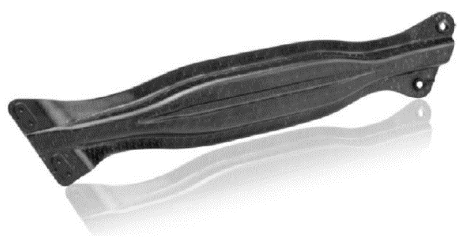
Within the “SpriForm” project, the Institute for Composite Materials in Kaiserslautern developed a process in which a continuous fiber-reinforced organic sheet is formed and overmolded in one process step [19]. A side impact door beam was developed that combines the high strength of continuous fibers with the design freedom of injection molding (Figure 1).

In the field of locally, continuously reinforced thermosets, extensive research was carried out for unidirectionally reinforced sheet molding compounds at the Karlsruhe Institute of Technology with focus on manufacturing [2] and characterization [20].

3. Optimization of Hybrid Structures

The optimization of reinforcement structures, within the hybrid structure, is often referred to as “load-path compatible design”. The first approach is an engineering estimation. For example, components subjected to bending loads can be divided into areas subjected to tensile, compressive and shear loads and the fiber reinforcement can be aligned accordingly.

A more precise option is stress analysis. Load paths can be defined using the finite element method (FEM). However, there is no generally valid definition of load paths [21]. Marhadi and Venkataraman summarize some approaches using two-dimensional continuum structures as an example. A common approach is the use of topology optimization to identify highly stressed areas. These areas are then reinforced with a high strength and/or high stiffness material within the hybrid structure.

This procedure concerning structures manufactured by the tailored fiber placement process is displayed in Figure 2 and explained in [3]. In the first step, topology optimization is carried out for the given design space and under the boundary conditions. The resulting structure is then assumed as the volume of the reinforcement structure. In a second step, material optimization is performed within this volume to determine the orientation of the anisotropic material. The final result is an optimized structure with optimized material orientation.

Strategies for optimizing topology and material orientation are presented in detail in Section 4 and Section 5.

4. Isotropic Topology Optimization

In the following, topology optimization in general will be explained, as it is an important element of the further developed strategy for optimizing cFRP in hybrid structures.

The aim of topology optimization is to find the best possible material distribution within a given design space, taking into account loads, boundary conditions and constraints. For structural-mechanical problems, the goal is usually to minimize the compliance of the structure.

Besides exact analytical optimizations [22], which mainly serve as reference solutions and are only known for simple standard problems, topology optimizers based on the FEM have become widely accepted. The three most commonly used methods are solid isotropic material with penalization (SIMP) [23], evolutionary structural optimization (ESO) [24,25] and the level set method [26]. For SIMP and ESO, in order to obtain the optimal solution for a limited volume of solid material, the basic idea is to decide for each element whether it should consist of void or solid material. Thereby solid material has the stiffness of the material used for the component and the void material has a stiffness of almost zero. This problem can only be solved directly with a very high numerical effort [26]. To reduce this effort in the SIMP algorithm, the discrete variables are replaced by continuous ones. A power-law interpolation is used to penalize intermediate densities to obtain a solution consisting of elements close to solid and void properties. In addition to SIMP, several empirical concepts that base on the idea of iteratively removing inefficient material exist. This basic idea is used in the ESO method [24]. The concept is extended in the BESO [11] where additionally efficient material can be added simultaneously.

In this paper, the BESO method is implemented because of its high-quality topology solutions, computational efficiency and ease of implementation [27]. It is explained in detail below. In order to maximize the stiffness of the structure, the strain energy must be minimized. This is expressed in Equation (1) where compliance $\mathrm{C}$ is the objective function that should be minimized. Here f and u are the applied force and displacement vectors.

$$\min : \mathrm{C}=\frac{1}{2}{\mathrm{f}}^{\mathrm{t}}\mathrm{u}$$

(1)

The BESO algorithm solves the optimization problem using a discrete variable, thus the elemental density can only be ${\mathrm{x}}_{\mathrm{i}}=1$ for solid elements or ${\mathrm{x}}_{\mathrm{i}}={\mathrm{x}}_{\min }$ for void elements. ${\mathrm{x}}_{\min }$ typically is a very small value, e.g., 0.001.

$${\mathrm{x}}_{\mathrm{i}}=1{ \mathrm{or} \mathrm{x}}_{\min }$$

(2)

The volume of all elements within the design space is constrained to the target volume ${\mathrm{V}}^{*}$ with the volume of each element ${\mathrm{v}}_{\mathrm{i}}$ and the relative density ${\mathrm{x}}_{\mathrm{i}}$.

$${\mathrm{V}}^{*}={{\displaystyle \sum }}_{\mathrm{i}=1}^{\mathrm{N}}{\mathrm{x}}_{\mathrm{i}}{\mathrm{v}}_{\mathrm{i}}$$

(3)

Whether an element consists of solid or void material depends on the element sensitivity ${\mathrm{a}}_{\mathrm{i}}$. The sensitivity for void or solid elements is calculated according to Equation (4).

$${\mathrm{a}}_{\mathrm{i}}=\{\begin{array}{cc}\frac{1}{2}{\mathrm{u}}_{\mathrm{i}}^{\mathrm{T}}{\mathrm{K}}_{\mathrm{i}}^1{\mathrm{u}}_{\mathrm{i}}& \mathrm{when} {\mathrm{x}}_{\mathrm{i}}=1\\ 0& \mathrm{when} {\mathrm{x}}_{\mathrm{i}}={\mathrm{x}}_{\min }\end{array}$$

(4)

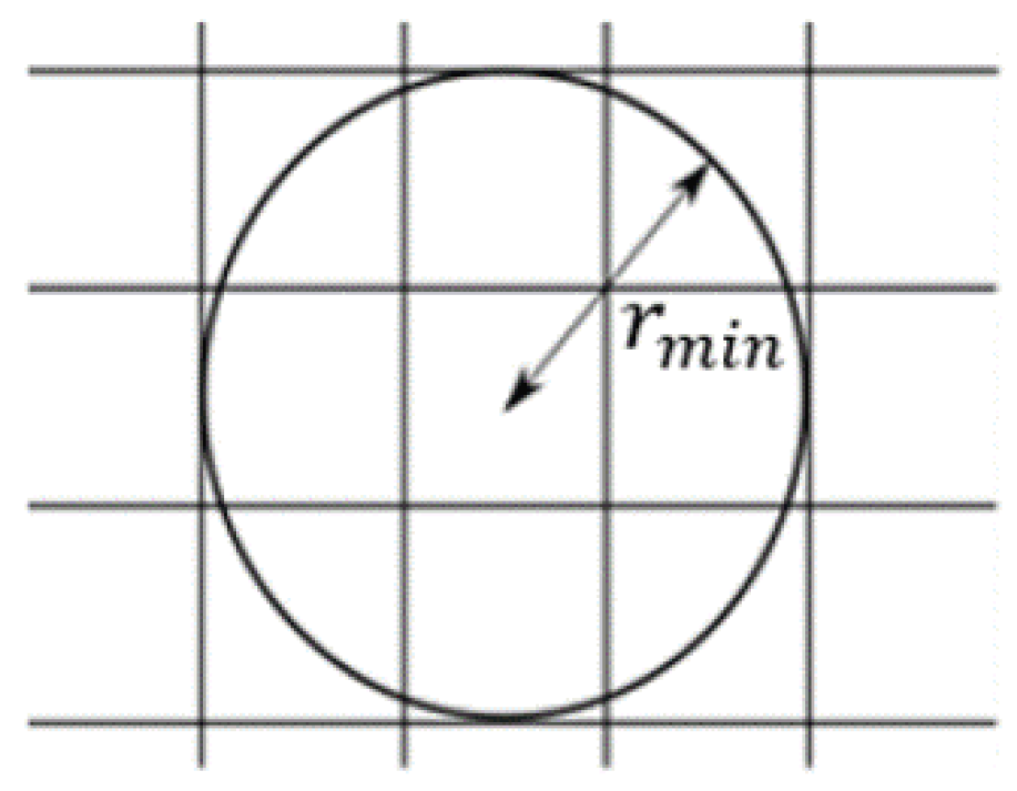
To avoid numerical instabilities, the calculated sensitivities are spatially filtered. For this purpose, there are several approaches [28]. In the following, the popular approach of Sigmund [29] is used. If element i lies within the filter-radius ${\mathrm{r}}_{\min }$ as displayed in Figure 3 the filtered sensitivities ${\mathrm{â}}_{\mathrm{i}}$ are calculated according to Equation (5).

$${\mathrm{â}}_{\mathrm{i}}=\frac{{{\displaystyle \sum }}_{\mathrm{j}=1}^{\mathrm{M}}\mathrm{w}\left({\mathrm{r}}_{\mathrm{ij}}\right){\mathrm{a}}_{\mathrm{j}}^{\mathrm{n}}}{{{\displaystyle \sum }}_{\mathrm{j}=1}^{\mathrm{M}}\mathrm{w}\left({\mathrm{r}}_{\mathrm{ij}}\right) }$$

(5)

The sensitivities are weighted linearly with the weighting function $\mathrm{w}\left({\mathrm{r}}_{\mathrm{ij}}\right)$ depending on the distance r and the defined filter-radius ${\mathrm{r}}_{\min }$.

$$\mathrm{w}\left({\mathrm{r}}_{\mathrm{ij}}\right)\{\begin{array}{cc}{\mathrm{r}}_{\min }-{\mathrm{r}}_{\mathrm{ij}}& \mathrm{for} { \mathrm{r}}_{\mathrm{ij}}<{\mathrm{r}}_{\min }\\ 0& \mathrm{for} {\mathrm{r}}_{\mathrm{ij}}\ge {\mathrm{r}}_{\min }\end{array}$$

(6)

To improve the convergence behavior, the sensitivities are additionally filtered over the optimization history. According to Equation (7), the mean value of the sensitivity of the current iteration k and the previous iteration k − 1 is formed. The weighting of the iterations can be adjusted to adapt to the convergence behavior.

$${\tilde{\mathrm{a}}}_{\mathrm{i}}=\frac{1}{2}\left({\mathrm{â}}_{\mathrm{i},\mathrm{k}}+{\mathrm{â}}_{\mathrm{i},\mathrm{k}-1}\right)$$

(7)

The optimization starts with a model that consists completely of solid material. Until the target volume ${\mathrm{V}}^{*}$ is reached the volume is reduced successively in every iteration depending on the evolutionary ratio $\mathrm{ert}$.

$${\mathrm{V}}_{\mathrm{k}}={ \mathrm{V}}_{\mathrm{k}-1}\left(1-\mathrm{ert}\right) \mathrm{if} {\mathrm{V}}_{\mathrm{k}}>{ \mathrm{V}}^{*}$$

(8)

To decide which elements consist of void or solid material a limit value for ${\mathrm{a}}_{\mathrm{th}}$ is defined. This threshold is chosen to achieve the target volume ${\mathrm{V}}_{\mathrm{k}}$ for the current iteration. If the element sensitivity is greater than the threshold value ${\mathrm{a}}_{\mathrm{th}}$, the element is assigned solid material.

$${\mathrm{a}}_{\mathrm{i}}>{ \mathrm{a}}_{\mathrm{th}}$$

(9)

If the sensitivity is below the threshold the element is assigned void material.

$${\mathrm{a}}_{\mathrm{i}}\le { \mathrm{a}}_{\mathrm{th}}$$

(10)

From iteration to iteration the volume ${\mathrm{V}}_{\mathrm{k}}$ is further reduced until the target volume ${\mathrm{V}}^{*}$ is reached. The optimization is terminated when the termination criterion (11) is fulfilled.

$$\mathrm{error}=\frac{\left|{{\displaystyle \sum }}_{\mathrm{i}=1}^{\mathrm{N}}\left({\mathrm{C}}_{\mathrm{k}-\mathrm{i}+1}-{\mathrm{C}}_{\mathrm{k}-\mathrm{N}-\mathrm{i}+1}\right)\right|}{{{\displaystyle \sum }}_{\mathrm{i}=1}^{\mathrm{N}}{\mathrm{C}}_{\mathrm{k}-\mathrm{i}+1}} \le \mathsf{\tau }$$

(11)

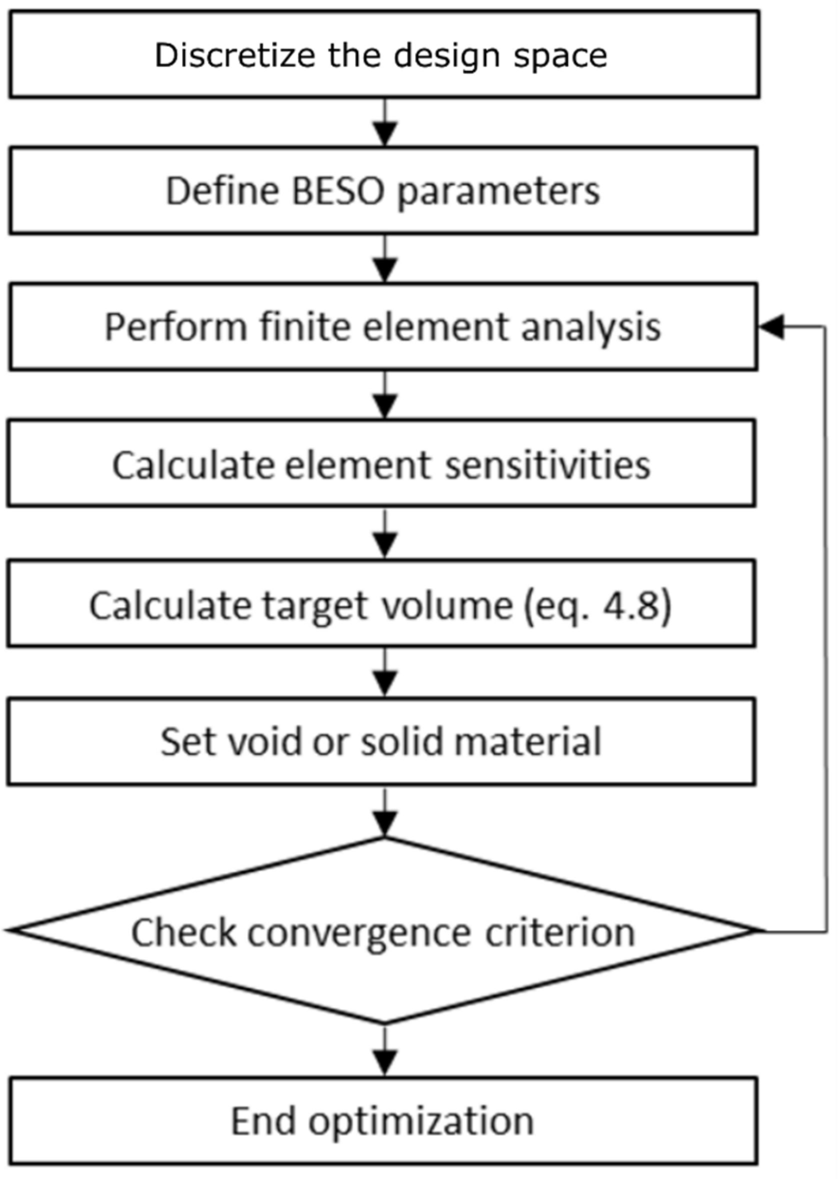
The complete procedure of the BESO method is summarized in Figure 4 as a pseudo flow chart.

5. Topology Optimization for Anisotropic Materials

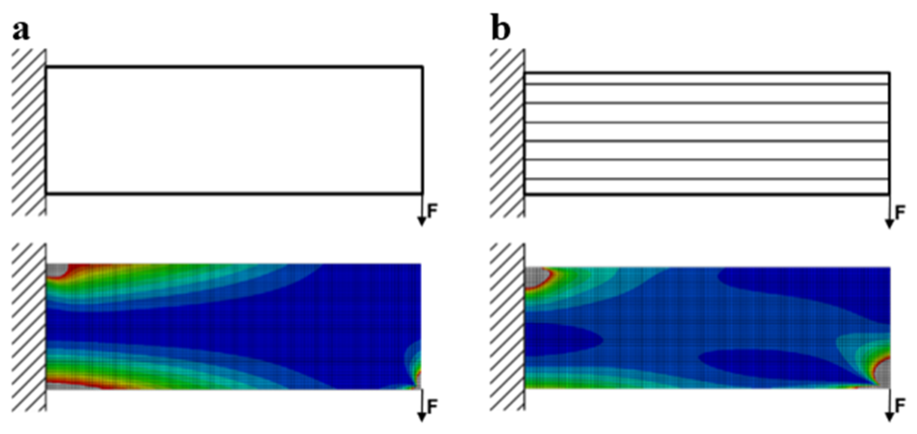
In topology optimization, the sensitivity for each element—in this case the strain energy—is evaluated for the assignment of void or solid material. If the anisotropy of the material is taken into account the strain energy distribution is different from that of an isotropic material, as Figure 5 shows for the example of a cantilever beam.

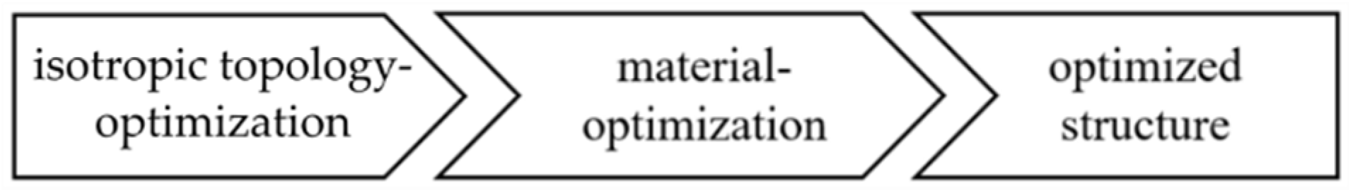
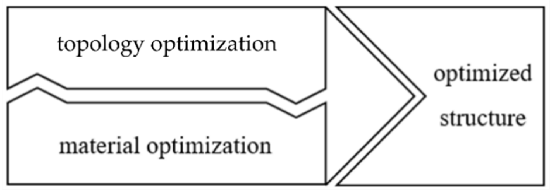
In order to take the fiber orientation of the anisotropic material into account, a fiber orientation must be assigned for every iteration. To find a reasonable orientation, a fiber angle optimization is performed in each iteration. The procedure for topology optimization is shown in Figure 6. The fiber angle optimization is carried out in conjunction with topology optimization and not sequentially (compare Figure 2).

Various approaches are applied to optimize the material orientation. In addition to the optimization of the orientation as a parameter [10], there is the analytical approach of orienting the material in the direction of the maximum principal stresses. For a sufficiently fine mesh, this method is a particularly efficient procedure because within a few iterations an optimal result can be found [7].

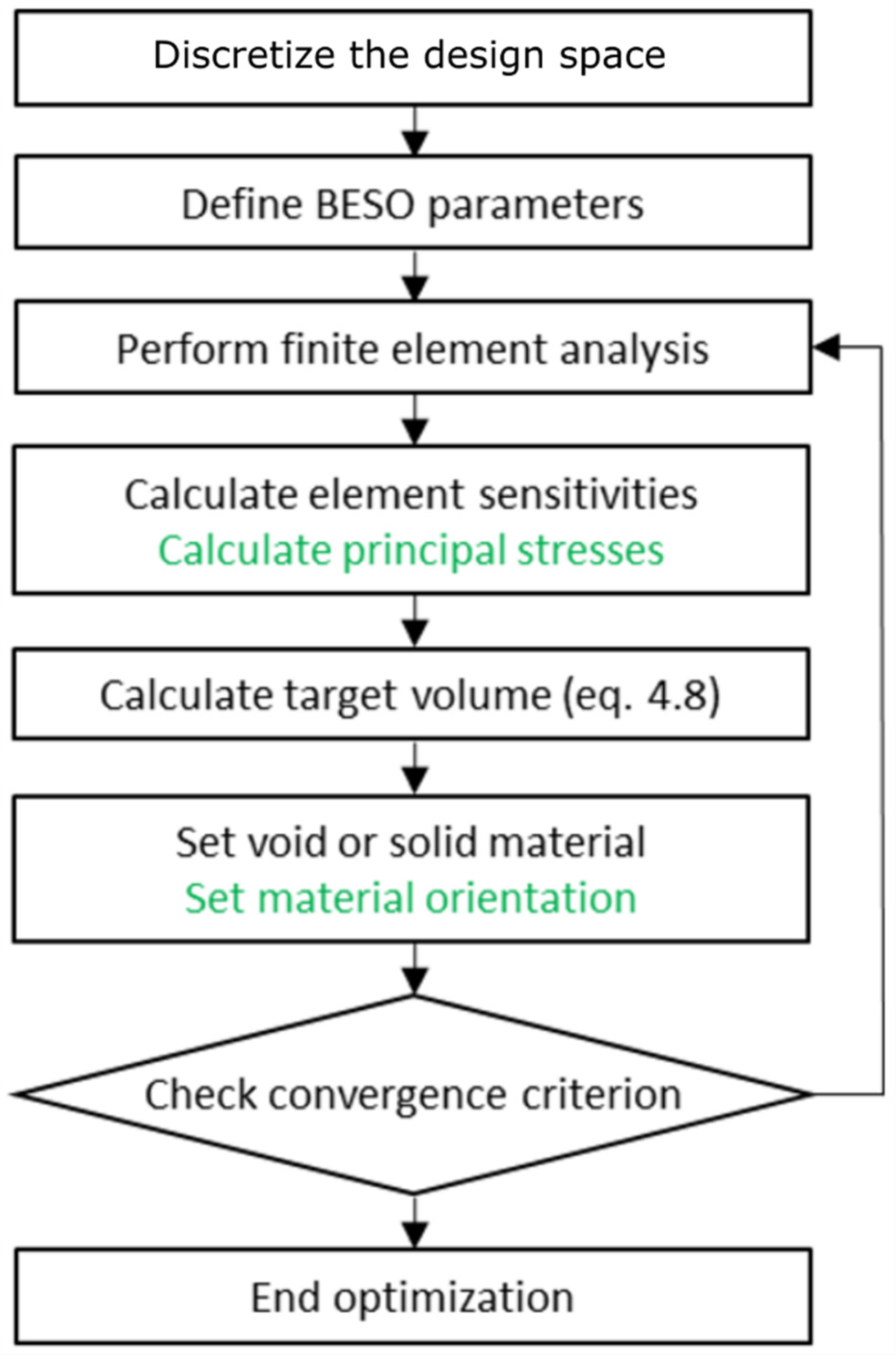
Approaches that combine material orientation in the direction of the principal stresses with the BESO method are already known from Safonov [8] and Yan [30]. Here an additional step is integrated into the BESO algorithm, which adapts the fiber-angle to the state of stress as shown in Figure 7 compared to Figure 4.

First, the direction of the maximum absolute principal normal stress is determined. Then the direction is assigned to the respective element as local material orientation. The local fiber orientation must be taken into account when calculating the sensitivity a_i. This is done by the stiffness matrix K_i (see Equation (4.4)).

6. Topology Optimization for Multiphase Structures

Hybrid structures consist of multiple materials with different stiffnesses. These different stiffnesses must be taken into account both within the FE calculation and in the calculation of sensitivities. For topology optimization, this means that the stiffness of the void elements is not nearly zero but corresponds to the stiffness of the base material (here sFRP). The stiffness of the solid material corresponds to that of the cFRP reinforcement material.

In the following, an approach of Huang and Xie [11] is included which allows the optimization of multiple materials using the BESO method. For the calculation of the sensitivities, Equation (4) is replaced by formula (12), which takes the different stiffnesses into account. ${\mathrm{E}}_{\mathrm{i}}$ is the the Young’s modulus of the respective material. For ${\mathrm{E}}_2\ll { \mathrm{E}}_1$ of the material and $\mathrm{p}\to \infty$ Equation (12) corresponds to Equation (4).

$${\mathrm{a}}_{\mathrm{i}}=\{\begin{array}{l}\mathrm{for} \mathrm{material} 1:\\ \frac{1}{2}\left[1-\frac{{\mathrm{E}}_2}{{\mathrm{E}}_1}\right]{\mathrm{u}}_{\mathrm{i}}^{\mathrm{T}}{\mathrm{K}}_{\mathrm{i}}^1{\mathrm{u}}_{\mathrm{i}}\\ \mathrm{for} \mathrm{material} 2:\\ \frac{1}{2}\frac{{\mathrm{x}}_{\min }^{\mathrm{p}-1}\left({\mathrm{E}}_1-{\mathrm{E}}_2\right)}{{\mathrm{x}}_{\min }^{\mathrm{p}}{\mathrm{E}}_1+\left(1 -{\mathrm{x}}_{\min }^{\mathrm{p}}\right){\mathrm{E}}_2}{\mathrm{u}}_{\mathrm{i}}^{\mathrm{T}}{\mathrm{K}}_{\mathrm{i}}^2{\mathrm{u}}_{\mathrm{i}}\end{array}$$

(12)

The number of different materials can be further increased according to [12]. The sensitivities are filtered both locally and historically according to Equations (5) and (7) in paragraph 4. The whole procedure is presented in more detail with numerical examples in [11].

7. Topology Optimization of Multiphase Anisotropic Reinforcement Materials

The application described in this paper is a material combination of material assumed to be isotropic (sFRP) and an anisotropic reinforcement material (cFRP). For sFRP local fiber orientations are not considered for simplification. Otherwise, an injection molding simulation would have to be performed in each iteration of the optimization in order to calculate the local fiber orientations within the sFRP. This would greatly increase the numerical effort. Therefore, the material properties of the sFRP have to be averaged. The error due to this simplification is relatively small compared to neglecting the anisotropy of the cFRP, due to the fact that the degree of anisotropy of the cFRP is much larger than the degree of anisotropy of the sFRP.

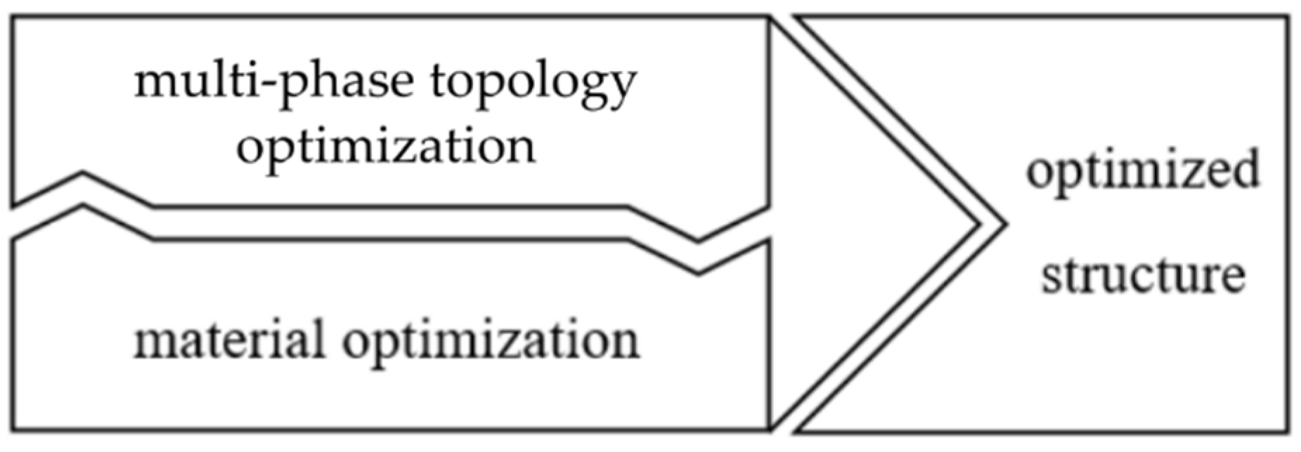
The algorithm described below was developed to optimize this material combination. In order to achieve this the most important material properties (anisotropy of cFRP and stiffness of sFRP) should be included within the optimization. Therefore, the optimization approaches presented in Section 5 and Section 6 are combined. The principle procedure is shown in Figure 8. The multi-phase topology optimization and the material optimization are carried out in each iteration. This simultaneously takes into account the stiffness of the base material and the anisotropy of the continuous fiber reinforcement.

In this approach the entire design space is filled with cFRP or sFRP. Therefore, for the target volumes of the continuous fiber-reinforced material ${\mathrm{V}}_1^{*}$ and the short fiber-reinforced material ${\mathrm{V}}_2^{*}$ the Equation (13) applies.

$${\mathrm{V}}_1^{*}+{ \mathrm{V}}_2^{*}=1$$

(13)

Fiber angle optimization is performed for the orthotropic material in each iteration (see Section 5) by evaluating the vector of absolute maximum principal normal stress for each element and setting it as the new fiber orientation for the next iteration.

The steps of this procedure are explained in detail below.

• Step 1: The available design space is discretized with an FE mesh and boundary conditions are specified.
• Step 2: BESO parameters V*, ert and p are defined.
• Step 3: Initialization of the model. A list of neighboring elements with elements and element distance r is created. The list of elements and distance between the elements is needed later for filtering sensitivities. This step only occurs at the beginning of the optimization and is not repeated in every iteration.
• Step 4: The FE calculation is carried out in Abaqus.
• Step 5: For every element, the vector of the maximum absolute principal stress is calculated from the result of the previous calculation. The local material coordinate system is oriented in the direction of the calculated vector.
• Step 6: From the result of the FE calculation the element sensitivities are calculated according to Equation (6.1). Afterward, the sensitivities are filtered spatially (Equation (4.5)) and over the optimization history (Equation (4.7)).
• Step 7: The target volume for the next iteration is calculated according to Equation (4.8) depending on ert and ${\mathrm{V}}_{\mathrm{k}}$ as long as V* is not reached.
• Step 8: cFRP and sFRP (which is assumed to be isotropic for simplification) are defined as solid and void material (see Equations (4.9) and (4.10))
• Step 9: The convergence criterion is monitored. If the convergence criterion (4.11) is fulfilled, the calculation is terminated. If it is not fulfilled, the process starts again at step 4.

8. Design Problem

To demonstrate the effect of considering anisotropy and stiffness of different materials the algorithm shown in Figure 7 and described in Section 7 is implemented in Abaqus using a Python script. A classic example is used to visualize the effects. A cantilever beam clamped on one side under vertical force load as displayed in Figure 9 serves as an example problem. The design space has a length of 150 mm and a height of 50 mm.

In order to evaluate the proposed method for different geometries and load cases, comparative calculations are carried out for the problems shown in Figure 10. In each case, the results of an isotropic topology optimizer are compared with those of the anisotropic and hybrid optimizer.

All examples are considered as plane problems and are discretized with S8R shell elements of edge length 2 mm. Small deformations are assumed for the FE calculation of the structures. Materials and displacements are calculated as linear elastic. The optimization aims to find the stiffest possible solution with a target volume V* = 40% of the continuous fiber-reinforced material. A filter radius of r_min = 6 mm is chosen for the filter function in Equation (5). The evolutionary ratio is set to ert = 1.5.

9. Results

The results for different algorithms with and without consideration of the anisotropy of the reinforcement material and the stiffness of the base material are compared qualitatively. The procedure shown in Figure 2 serves as a reference, where first a topology optimization for an isotropic material and then a material optimization is performed.

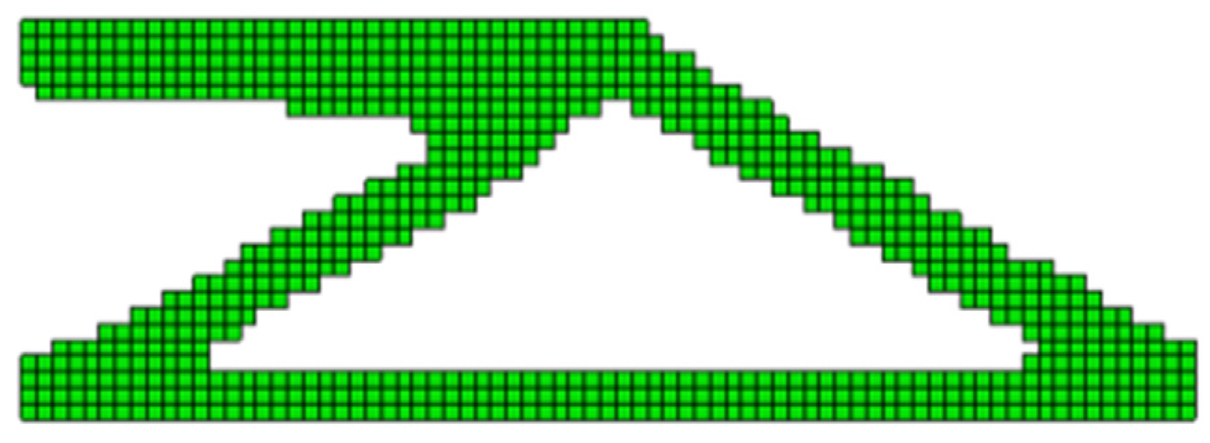
The BESO algorithm in Section 4 is used for this purpose. For the solid material, an isotropic material with Young’s modulus of ${\mathrm{E}}_1=12,500 \mathrm{MPa}$ is assumed. The void stiffness is almost zero with ${\mathrm{E}}_2=0.001 \mathrm{MPa}$. The result of the isotropic optimization is the typical truss structure in Figure 11.

In the next step, the anisotropy of the cFRP reinforcement material is included within the optimization. For the solid material a stiffness ${\mathrm{E}}_{1\Vert }=100,000 \mathrm{MPa}$ in fiber direction and ${\mathrm{E}}_{1\perp }=10,000 \mathrm{MPa}$ in transverse fiber direction is assumed. These values correspond to a unidirectional C-fiber reinforced plastic. The stiffness of the void material is still assumed to be almost 0, ${\mathrm{E}}_2=0.001 \mathrm{MPa}$. For this purpose, the procedure is described in Section 5. In each iteration, in addition to the assignment of void and solid material, the material orientation for every element is adapted according to the respective principal normal stress.

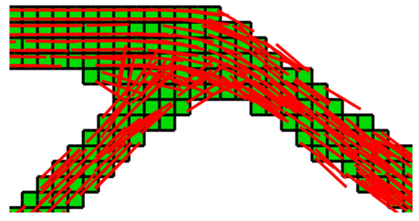
The material orientation for solid elements of the optimized structure can be seen in Figure 12. The fiber-orientation follows the direction of the struts of the reinforcement structure. This generally applies to all optimization results presented in the following. The consideration of the anisotropy of the solid material tends to lead to simpler structures with fewer struts and thus fewer junctions (Figure 13). This happens because multi-axial stress states occur in the nodal regions, which leads to low stiffness in the anisotropic material.

In a final step, both the anisotropy of the reinforcement material and the stiffness of the base material are considered concurrently. For this purpose, as explained in Section 7, the approaches from Section 5 and Section 6 are combined. For the solid material the stiffnesses ${\mathrm{E}}_{1\Vert }=100,000 \mathrm{MPa}$ in longitudinal direction and ${\mathrm{E}}_{1\perp }=10,000 \mathrm{MPa}$ transverse to the fiber direction is assumed. An isotropic material with a stiffness ${\mathrm{E}}_2=12,500 \mathrm{MPa}$ is assumed as base material, which corresponds to a highly filled sFRP (e.g., PA6-GF40).

In the following, the influence of the stiffness of the base material is quantitatively estimated. Comparative calculations with different stiffnesses for the base material are presented.

The result in Figure 14 shows that for such stiff base materials, by taking into account the stiffness of the void elements, struts in the mainly shear-loaded area can be avoided. This results in a much simpler reinforcement structure compared to the optimization result in Figure 11.

Figure 15 shows exemplary results of the optimization for Young’s modulus of the base material of (a) 2500 MPa, (b) 7500 MPa and (c) 12,500 MPa. The results show that as Young’s modulus of the base material increases, the more reinforcing material is transferred from the shear-loaded areas to the tensile and compressive loaded areas. The results for different optimization algorithms are summarized in

Table 1. Comparison of the performed optimizations. As reference a cantilever beam made of sFRP with an ${\mathrm{E}}_2=12,500 \mathrm{MPa}$ (a) is used here. A significant increase in stiffness can be achieved by inserting a continuous fiber reinforcement (${\mathrm{E}}_{1\Vert }=100,000 \mathrm{MPa}$, ${\mathrm{E}}_{1\perp }=10,000 \mathrm{MPa}$). For (b) the reinforcement structure was optimized using a BESO algorithm for isotropic materials. Variant (c) shows the result when the anisotropy of the fiber reinforcement is taken into account. In (d), both the anisotropy of the fiber reinforcement and the stiffness of the injection molding material were included in the optimization. This allows to increase the stiffness even further for the same amount of material.

Material	Optimization	Result	Stiffness Increase Factor
a sFRP without continuous fiber-reinforcement	-		reference
b sFRP with continuous fiber-reinforcement	Standard isotropic BESO algorithm neglecting stiffness of sFRP		approx. 5.5
c sFRP with continuous fiber-reinforcement	Anisotropic BESO algorithm with concurrent fiber-angle optimization neglecting stiffness of sFRP		approx. 5.5
d sFRP with continuous fiber-reinforcement	Anisotropic BESO algorithm with concurrent fiber-angle optimization considering the stiffness of the base-material		approx. 6.1

. In reference a, the cantilever beam described in Section 8 consists entirely of sFRP with a modulus of elasticity of 12,500 MPa. By substituting 40% of the part volume with a continuous fiber reinforcement (${\mathrm{E}}_{1\Vert }$ = 100,000 MPa, ${\mathrm{E}}_{1\perp }$= 10,000 MPa), the stiffness of the part can be significantly increased. In case b the layout of the reinforcement was optimized using an isotropic topology optimizer without considering the stiffness of the base material. Thus the stiffness of the component can be increased by a factor of 5.5.

Additionally, the anisotropy of the reinforcing material is taken into account in c. This also results in an increase in component stiffness by a factor of 5.5, so no further increase is achieved, but a qualitatively simpler structure with fewer struts could be reached.

Finally, the different material properties were completely modeled during the optimization in d. This includes the anisotropy of the continuous fiber-reinforcement as well as the stiffness of the base material. Thus, the component stiffness can be increased by a factor of 6.1 compared to the reference. In addition, the structure is further simplified.

The influence of the stiffness of the base material will be quantitatively estimated in the following. Comparative calculations with different stiffnesses for the base material are presented. The stiffness of the optimized structure is calculated for a base material with various elastic moduli, in order to evaluate the influence on the stiffness. The results are compared to the stiffness of the reference optimization result in Figure 11. To ensure comparability, after the optimization of the reference for isotropic material, a fiber angle optimization is performed and the anisotropic material is assigned. Additionally, the material properties of the base material of the corresponding optimization calculation are assigned.

Figure 16 shows the stiffness of various optimized structures as a function of the respective Young’s modulus of the base material. As a reference, the stiffness of a reinforcing structure that has been optimized without considering the anisotropy and stiffness of the base material is given (compare Table 1b).

With increasing Young’s modulus of the base material, the structures not only differ more and more clearly from the reference in terms of quality (see Figure 15), but the stiffness also increases more when the material properties are taken into account. The higher the Young’s modulus of the sFRP the less cFRP-material is needed to carry the shear load between tension and compression loaded regions. Therefore more cFRP can be located at the top and at the bottom of the cantilever beam and the moment of inertia of the cFRP-structure is increased.

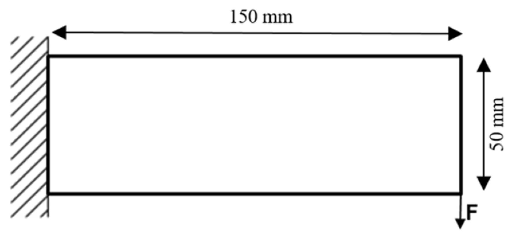
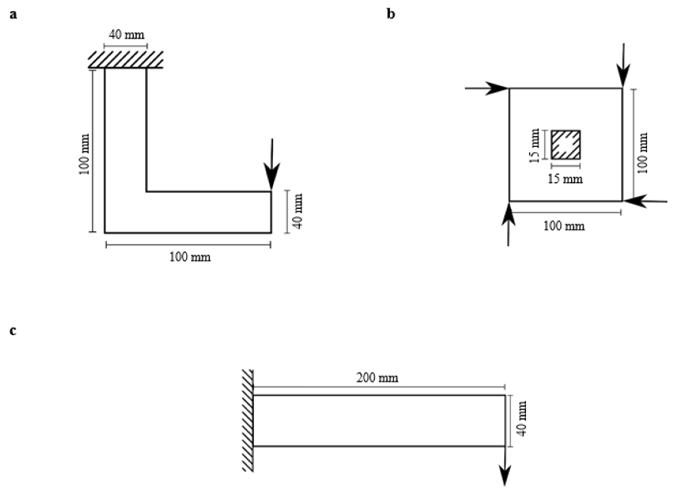
To demonstrate the effect of the new hybrid anisotropic optimizer compared to an isotropic optimizer, the load cases shown in Figure 10 are calculated with the boundary conditions given in Section 8. The longitudinal stiffness of the cFRP material is ${\mathrm{E}}_{1\Vert }$ = 100,000 MPa. The stiffness of the sFRP assumed to be isotropic is ${\mathrm{E}}_2$ = 20,000 MPa.

Figure 17 shows the results for these three load cases. It can be seen that both the differences in resulting topology and achievable stiffness between the optimization algorithms strongly depend on the particular geometry and load case. In example a, there is only a 2.8% increase in the achievable stiffness. In contrast, the resulting topologies are very different. Less shear-loaded struts result as a solution because, compared to the single-phase, isotropic optimizer, the shear stiffness of the sFRP is already taken into account during optimization. The material is arranged more strongly in tension and compression loaded areas instead. In the case of the very stiff sFRP used here (${\mathrm{E}}_2$ = 20,000 MPa), this even results in the continuous fiber structure no longer forming a continuous structure between force introduction and fixed constraint. B shows the square design domain with a central square rigid support [21]. By taking into account the hybrid and anisotropic material properties, the stiffness can be increased by 6.3%. The isotropic topology optimizer results in a truss-like solution. In contrast, the hybrid, anisotropic optimizer does not show any pronounced junction points. This leads to a more uniform curvature of the cFRP material. Example c is a cantilever beam with an aspect ratio of 5. Here, an increase in stiffness of 25.5% can be achieved compared to the isotropic topology optimizer. The resulting reinforcement structure has no connection at all between tensile and compressive loaded regions of cFRP. The shear load is transferred entirely by sFRP. Thus, cFRP can be located entirely in the uniaxially loaded areas.

10. Discussion

The comparison of the different algorithms has shown that the FE-calculations within the optimization have to be carried out with the parameters of the later used materials. In order to achieve converging solutions for non-isotropic, non-single-phase problems, the optimization algorithm described in Section 4, Section 5 and Section 6 were combined to a new approach which is explained in Section 7. It was shown that the consideration of the material properties leads to significant differences in the optimization results.

Figure 16 outlines how much potential of hybrid material combinations is lost with regard to the achievable stiffnesses for the same material input. Especially high stiffnesses of the base material lead to large differences. At a stiffness of the base material of 20,000 MPa (e.g., PA6-CF30) the difference is 17%. This is particularly important since local continuous fiber-reinforcements are mainly used when an increase of the fiber volume fraction of sFRP is no longer sufficient to achieve the required mechanical properties.

Besides the quantitative differences in the achievable stiffnesses, there are also qualitative differences (see Figure 11, Figure 13 and Figure 14). Optimization results that take into account the anisotropy of the cFRP and stiffness of the base material tend to have fewer struts. Therefore they are less complex to manufacture, which allows a more economical production of hybrid structures.

In the calculations presented, the stiffness of the cantilever beam is always the goal of the optimization. In the following steps, the strength should also be considered. It is to be expected that in addition to the strength of the continuous fiber reinforcement and the base material, the interface between the two materials is also of great importance.

For hybrid problems, the base material and the continuous fiber reinforcement are included in the optimization so far. Additionally, the multi-material approach according to Huang and Xie [11] can be extended by any number of materials. Thus, materials with different Young’s moduli (e.g., different fiber volume fractions of the continuous fiber reinforced plastic) could be included within the optimization. By allowing different materials the stress level within the structure could be further uniformed.