Article

Obtaining the Dimensions and Orientation of 2D Rectangular Flakes from Sectioning Experiments in Flake Composites

by
Thanasis D. Papathanasiou
1,*,
Andreas Tsiantis
1 and
Yanwei Wang
2,3
1
Department of Mechanical Engineering, University of Thessaly, 383-34 Volos, Greece
2
Department of Chemical and Materials Engineering, School of Engineering and Digital Sciences, Nazarbayev University, Nur-Sultan 010000, Kazakhstan
3
Laboratory of Computational Materials Science for Energy Applications, Center for Energy and Advanced Materials Science, National Laboratory Astana, Nur-Sultan 010000, Kazakhstan
*
Author to whom correspondence should be addressed.
J. Compos. Sci. 2022, 6(5), 142; https://0-doi-org.brum.beds.ac.uk/10.3390/jcs6050142
Submission received: 30 March 2022 / Revised: 28 April 2022 / Accepted: 9 May 2022 / Published: 13 May 2022
(This article belongs to the Special Issue Feature Papers in Journal of Composites Science in 2022)

Abstract

:
Recently, we developed and reported the statistical validity of two methods for determining the planar aspect ratios of two-dimensional (2D) rectangular flakes in composites from the statistics of intersection lengths: one method is based on the maximum intersection length, and the other on the average intersection length. In this work, we show that these methods are valid and robust not only for flakes having isotropic, random in-plane orientations, but for the more general situations of planar orientations ranging from unidirectional (misalignment angle ϵ = 0 ), to partially aligned ( 0 < ϵ < π / 2 ), to flakes of isotropic, random-in-plane orientations ( ϵ = π / 2 ). We prove, by Monte Carlo simulations and by numerical sectioning experiments, the validity of the proposed methods for characterizing the extent of the partial alignment (the misalignment angle ϵ ) of 2D rectangular flakes in composites, based again on the statistics of the intersection lengths; this information can be obtained from cross-sections of composite samples used in optical or electron microscopy or using tomographic imaging techniques. The performance of these techniques was tested using blind experiments in numerically sectioned composites which contained up to 10 6 individual flakes, and was found to be very good for a wide range of flake aspect ratios.

1. Introduction

Two-dimensional (2D) microstructures, e.g., flakes, plates, tapes and ribbons, offer unique properties as reinforcements for composite materials, and composites with such planar reinforcements already received considerable attention in the 1950s, as summarized in several early reviews [1,2,3,4]. By incorporating glass, silicon carbide (SiC), graphite, mica, clay or metallic flakes into a polymer matrix, flake-filled polymeric composites may offer significant processing and property advantages, such as high-dimensional stability and low warpage in molding [5,6], uniform in-plane mechanical properties and superior mechanical performance for 2D loading [2,3,7]; and nonstructural advantages, such as electrical insulating [8], conductive coating (with metallic flakes) [9], enhanced thermal conductive performance [10], corrosion protection [11], sound insulation [12] and appearance and color control [13]. In recent years, research activities on flake composites have been further boosted by the advent of and advances in graphene flakes and other 2D layered materials as fillers [14,15,16,17,18,19,20,21].
Flake-filled composites have found uses as barrier materials for food and electronics packaging [22,23,24,25,26], where the objective is to hinder the diffusion of oxygen, CO2 or other vapors to and from a container while maintaining all the advantages of formability and design afforded by plastic materials. One additional advantage is that the geometries in which such barrier property improvement is to be realized are very similar to those in which the mechanical superiority of flake-filled systems is also evident, such as in plates, shells, cylinders and pipes; therefore, barrier improvement can be combined with good mechanical performance [22,23,24,25,26,27]. We have recently demonstrated [28,29] that, in the particular case of flakes of rectangular shape, the barrier efficiency of the resulting composite is a very strong function of the planar flake aspect ratio. The assumption of a certain shape, size or orientation is very common in the technical literature, especially when models for material properties are developed and/or when numerical simulations are carried out. However, it introduces a serious source of uncertainty, since the actual shapes and sizes of flakes in composites are usually not known a-priory. Therefore, the development of techniques for determining the dimensions of flake particles (in our case, the width and aspect ratio) from information that can be readily obtained experimentally is highly desirable.
Besides size and shape, knowledge of particle orientation is essential for correct prediction of the properties of composites which incorporate slender particles, such as fibers and flakes. In fact, obtaining the orientation of elongated particles in composite materials is a long-standing problem in composite science. Composite parts are typically imaged by physically sectioning the composite and observing a fracture surface or a polished cross-section using optical or scanning/transmission electron microscopy [30,31,32,33], or by tomographic sectioning techniques. This problem has been handled in sufficient detail in cases of fibrous composites, in 2D cross-sections of which the fibers appear as circles or ellipses, depending on their orientations with respect to the sectioning plane [34,35,36,37,38,39,40]. In the case of composites in which the reinforcing particles have a thin, planar shape (flake composites), flake orientation can be especially difficult to characterize experimentally. As noted by Gaska et al. [26], while the cryo-fracturing method is widely used to expose fillers (graphene flakes in their study) in thermoplastic nanocomposites, the alignment was not clearly visible when only cryo-fracturing was used. In general, the problem of obtaining the orientation of flakes from data obtained in a typical sectioning experiment has not been solved yet.
Recently, we have presented two methods for the determination of the lateral dimensions of thin rectangular flakes [41] from the distribution of lengths of the lines representing the intersection of flakes with a sectioning plane. The first method finds the aspect ratio r from the diagonal D of the rectangle, assuming that D max ( H ) , subject to a user-defined accuracy threshold, where H is the vector of intersection lengths. The second method finds the aspect ratio r from the average length H a v of the flake cross-sections and is valid in the range 1 < r < 15 . These methods are extended in this work to systems in which the flakes assume random in-plane alignment in the interval [ ϵ , + ϵ ] , with 0 < ϵ < π / 2 . In addition to demonstrating that the methods are valid and robust for flakes having random in-plane orientations, we develop here a methodology that allows for the determination of the extent of flake misalignment in partially-aligned flake systems from knowledge of the statistics of intersection lengths. The performance of our techniques was tested using blind experiments in numerically sectioned composites and was found to be very good.

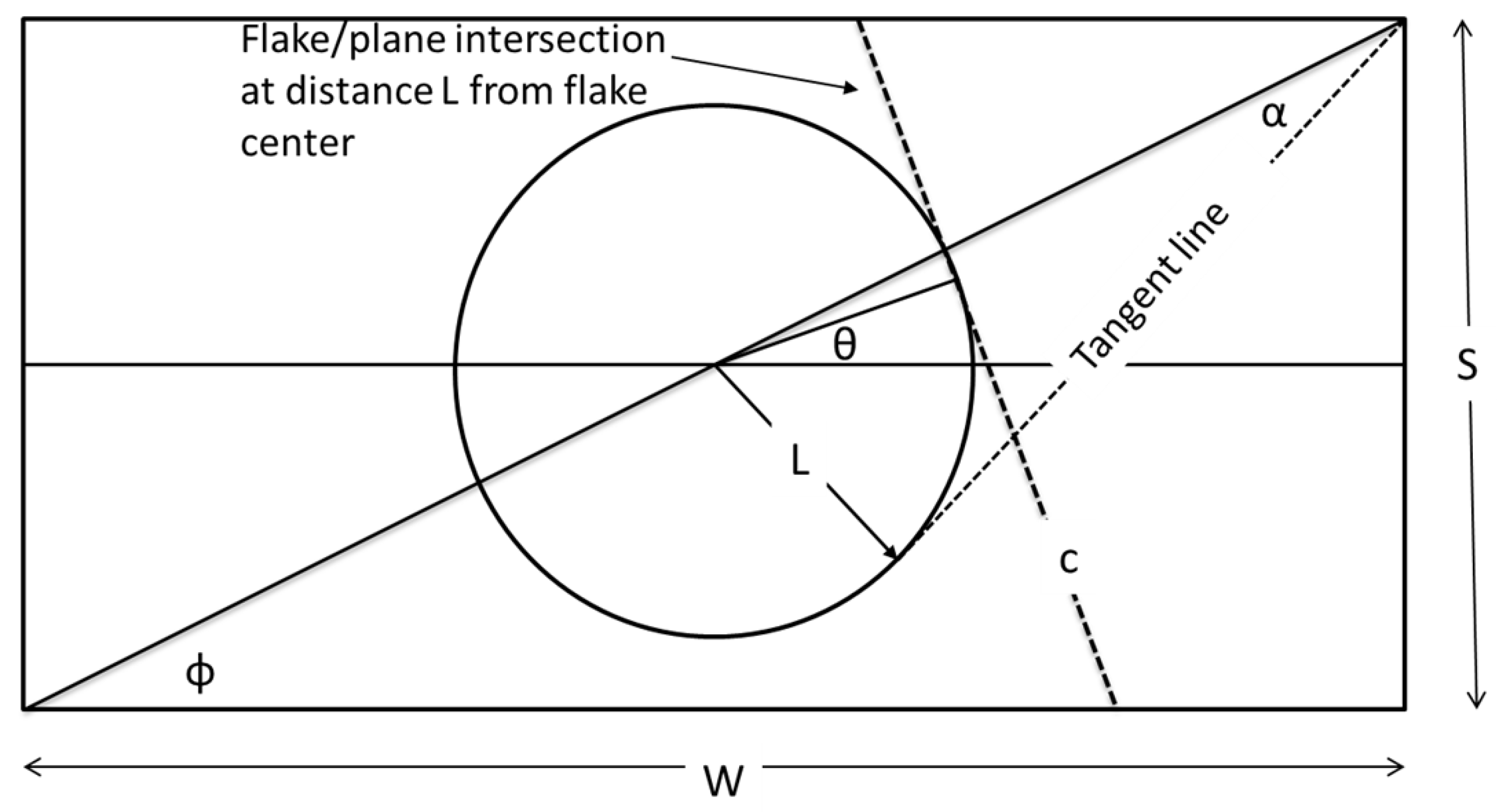
2. Theoretical Model and Methods

This work focuses on partially-aligned 2D rectangular flakes in composites. The flakes are of rectangular shape of and of uniform size. We denote by S the short side and by W the long side of the rectangle, its aspect ratio r = W / S and diagonal length D = S 2 + W 2 . Flakes planes are parallel to the X-Y plane and have in-plane orientations, described by the angle θ varying in the interval [ ϵ , + ϵ ] in the X-Y plane. Figure 1 presents top views of the sample geometries showing flakes with the aspect ratio r = 3 , oriented at different intervals [ ϵ , + ϵ ] around the y-axis.
Three-dimensional representative volume elements (3D RVEs) containing flakes were generated using an in-house random sequential addition (RSA) algorithm, as described in Ref. [42], wherein the flakes are allowed to assume random in-plane orientations. A fail-safe mechanism is implemented by which the calculation stops if a specified number of attempts ( O ( 10 9 )) is exceeded. More details on geometry generation and numerical sectioning are reported in Ref. [41]. In the present work, we studied flakes with partial in-plane alignment with the orientation angle in the interval [ ϵ , + ϵ ] , where 0 < ϵ < π / 2 . In comparison, Ref. [41] focused on the two limiting cases of ϵ = 0 (i.e., flakes are unidirectional) and ϵ = π / 2 (i.e., flakes have isotropic, random in-plane orientations).
On the assumptions that flakes are of rectangular shape and flakes in different layers are parallel to each other, we note that these assumptions are very much consistent with the current state-of-the-art in the area of flake composites. Due to their planar shape, flakes in a composite produced through a flow-processing technique will be expected to assume orientations parallel to each other, with only minimal out-of-plane misalignment [43]. This will be more true for flakes deposited using coating or lithographic techniques. However, we are not aware of any experimental data that will support or disprove this hypothesis.
Numerical samples of 3D RVEs were generated by setting the value of flake number density N / Δ V and flake width S and aspect ratio r. Numerical sectioning experiments (Figure 2) were carried out to obtain the H statistics—histogram, H a v for each sample and H for an ensemble of K = 10 samples in each case. In Figure 2 the process is illustrated. It is obvious that the distance between the cutting planes must be > 2 W to avoid counting the same flake twice between cutting planes.
In the following, we investigate the case in which the flakes show a preferred orientation, described by the angle θ varying in the interval [ ϵ , + ϵ ]. Since the angle formed between the sectioning plane and the long axis of the rectangle is π / 2 + θ , for ϵ = 0 , we derive the unidirectional case, in which all flakes are oriented with their long axis perpendicular to the sectioning plane, and for ϵ = π / 2 , we recover the case of random-in-plane orientations examined earlier. Our earlier analysis has shown that the intersection lengths can be calculated as [41]:
  • 0 < θ < θ 1
    H = S cos ( θ )
  • θ 1 < θ < θ 2
    H = D 2 L cos ( ϕ θ ) cos ( ϕ θ ) sin ( 2 θ )
  • θ 2 < θ < θ 3
    H = W sin ( θ )
  • θ 3 < θ < θ 4
    H = D + 2 L cos ( ϕ + θ ) cos ( ϕ + θ ) sin ( 2 θ )
  • θ 4 < θ < π
    H = S cos ( θ )
where θ 1 = π / 2 α ϕ , θ 2 = π ϕ arccos ( 2 L / D ) , θ 3 = π / 2 α + ϕ and θ 4 = π / 2 + α + ϕ , and the two angles α = arcsin ( 2 L / D ) and ϕ = arctan ( S / W ) = arctan ( r 1 ) as shown in Figure 3. The algorithm described in Equations (1)–(5) is directly applicable with the provision that the angle ( θ ) takes random values in the interval [ ϵ , + ϵ ], where 0 < ϵ < π / 2 .

3. Results and Discussion

Figure 4 shows the distribution of intersection lengths, for flakes of aspect ratio r = 2 , 5 , 10 and at various ϵ values. In each case, 2 × 10 5 random pairs of (L, θ ) were used in obtaining the histograms. It is clear that, as in the case of random-in-plane orientations, the highest frequency of intersection lengths coincides with the short side of the rectangle ( H / S = 1 ), and this offers a means of determining S. Contrary to what was observed in [41], for the case of ϵ = π / 2 , there is no secondary peak in the H-histogram.
It is evident from Figure 4a that max ( H ) is a function of ϵ , and it is clear from Figure 4b that max ( H ) is independent of the aspect ratio r. These observations form the basis of a method for the determination of ϵ from max ( H ) , as described in the following subsections.

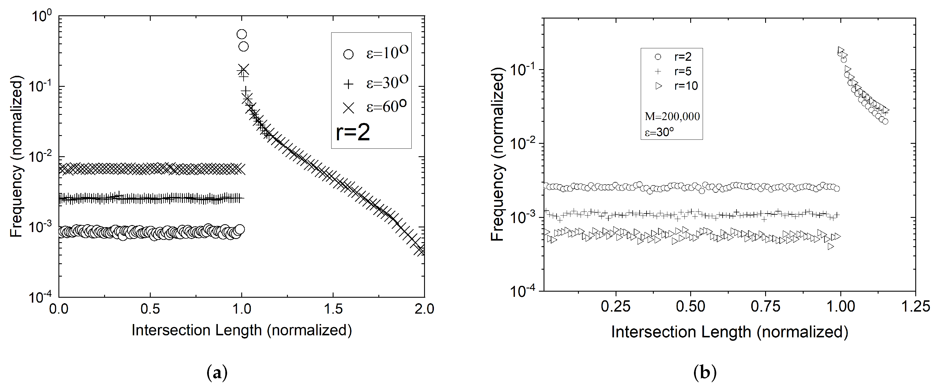
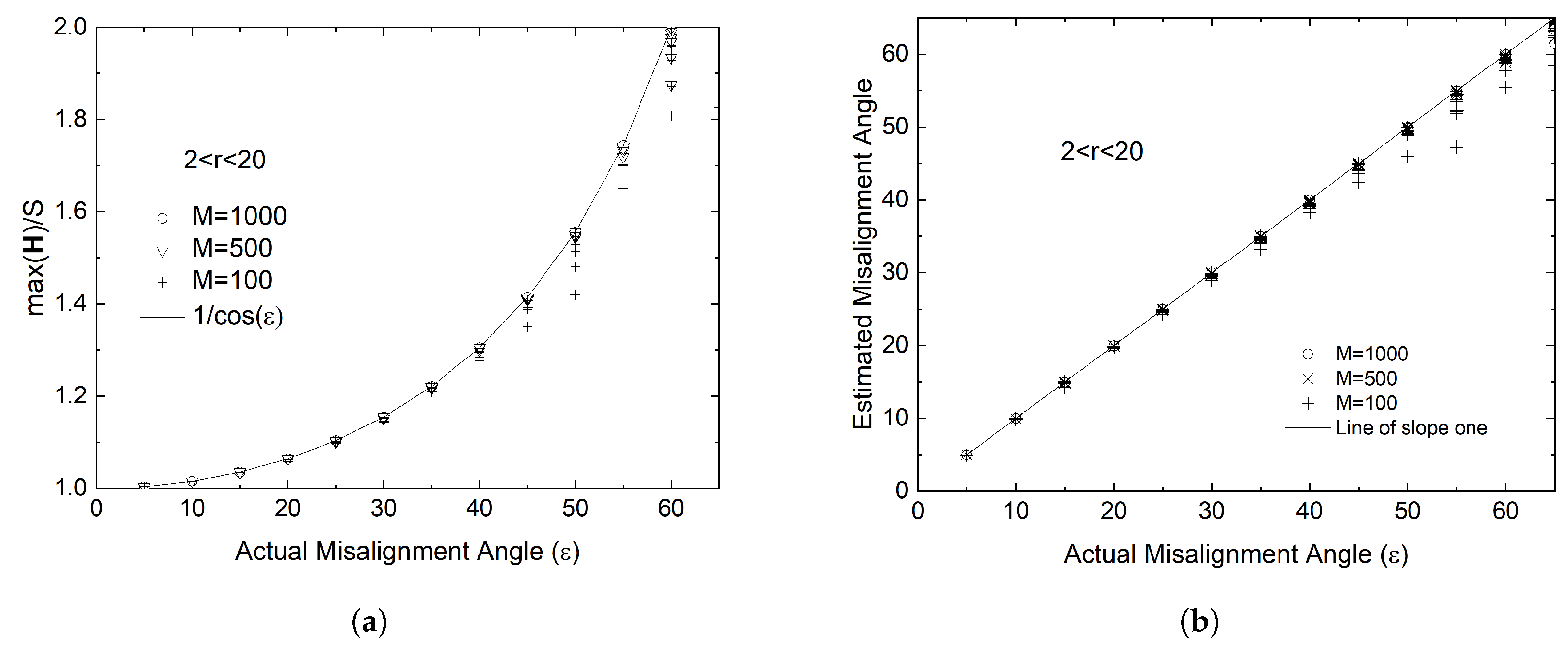
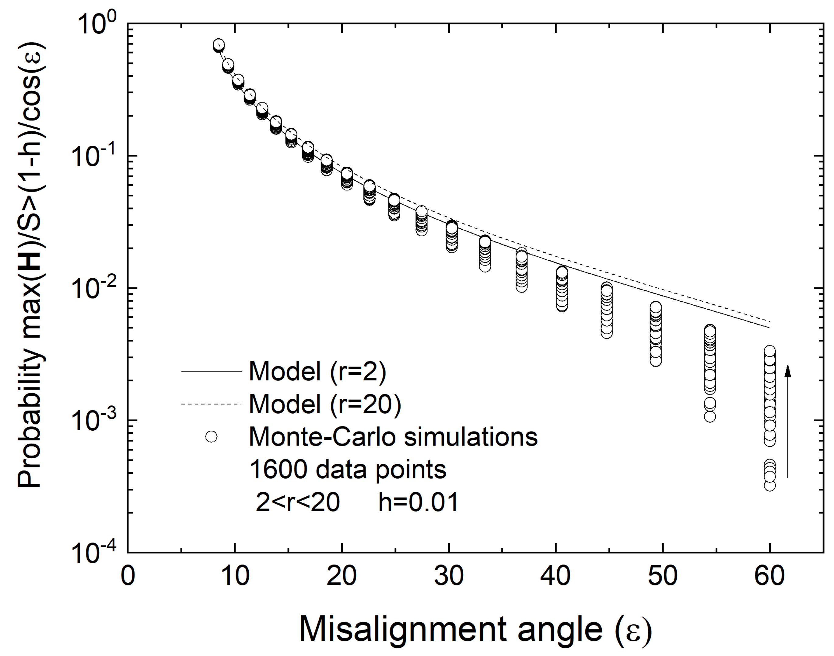
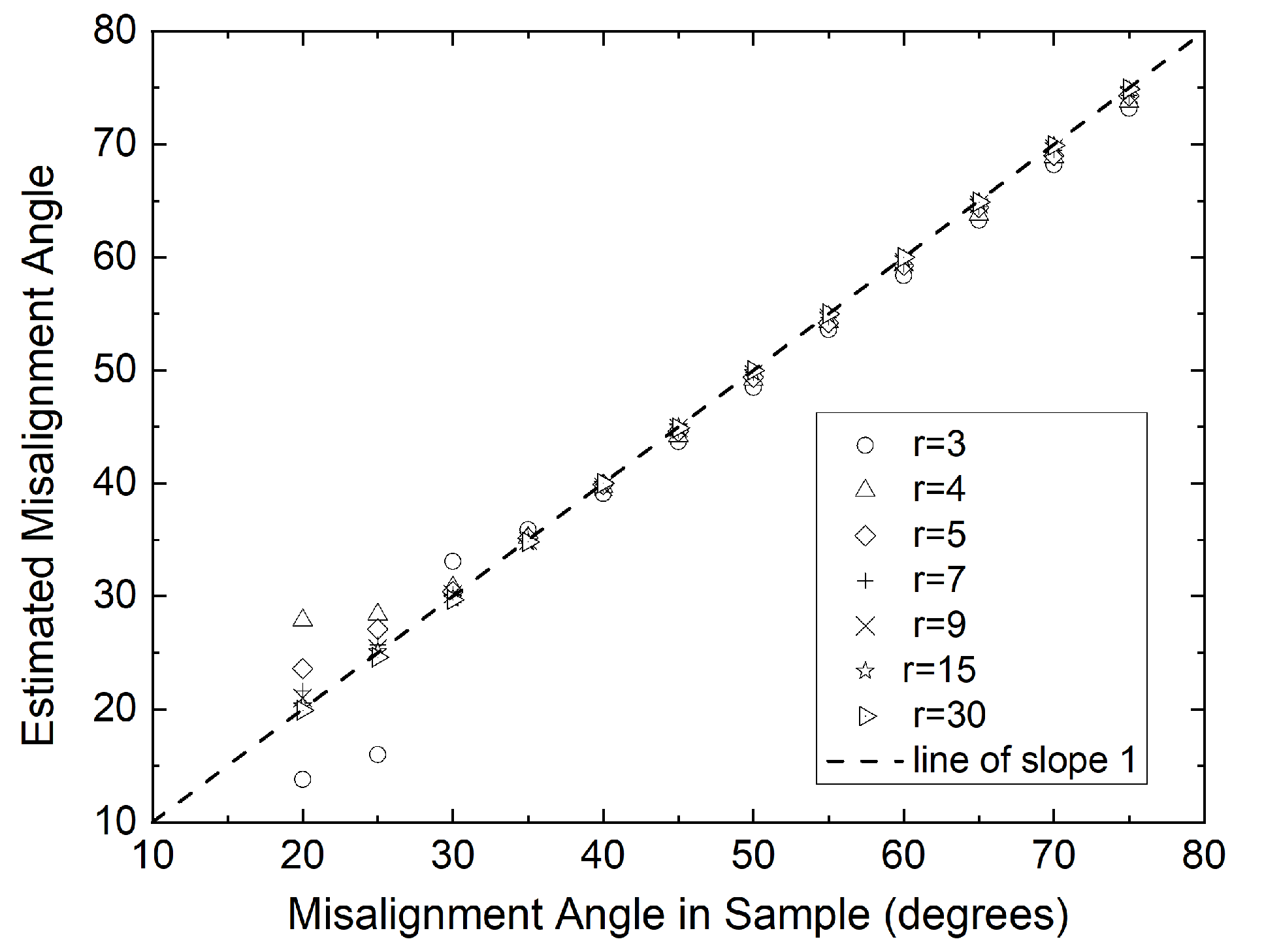
3.1. Determination of Partial Flake Alignment from the Maximum Intersection Length max(H)

With reference to Figure 3, it can be seen that for 0 < ϵ < ω , where ω = arccos ( S / D ) = arccos 1 / 1 + r 2 is the angle between the vertical and the diagonal of the rectangle, the cutting plane intersects the two opposite long sides of the rectangle, and it will be H = S / cos θ , as in Equations (1)–(5). For an infinitely large sample size, the maximum value of H will occur for the lowest value of cos θ . Since ϵ < θ < ϵ , it will be max ( H ) = S / cos ϵ , which is only a function of ϵ . This result is only valid for ϵ < ω ; however, this is not a very restrictive requirement, since for r = 1 , ω = 45 , and for r = 2 , ω = arccos ( 1 / 5 ) = 63 , increasing further as r increases. For r = 5 , 10 and 20, the values of ω are 78 . 7 , 84 . 3 and 87 . 2 respectively. For the following discussion, and for the sake of brevity, we will use the above result for all flakes of r 2 and for ϵ 63 . However, the same approach can be used for larger values of ϵ as long as the range of acceptable flake aspect ratios is appropriately reduced. For r 5 , for example, the method is suitable for all ϵ 78 . 7 . Obviously, for slender ribbons, the approach is valid for all ϵ < π / 2 ; in that case we recover an approach similar to that used to determine the extent of misalignment in long cylinders [34,44].
We have carried out simulations based on the model of Equations (1)–(5), supported by numerical sectioning experiments, in order to investigate the practical utility of such a correlation between max ( H ) and ϵ . The results are shown in Figure 5. As expected, with increasing M, the data approaches the curve max ( H ) = S / cos ϵ , which, as elaborated above, is the maximum achievable intersection length at each level of ϵ . For a finite sample size M, it will be max ( H ) S / cos ϵ , subject to a user-defined accuracy threshold. This can be used to derive an estimate of the maximum misalignment angle as
ϵ e s t = arccos max ( H ) / S
This approach will always underestimate the actual misalignment angle ϵ . Figure 5a gives an appreciation of the sample size needed to achieve this. It is clear that, as a result of the restricted range of θ , the probability of finding acceptable max ( H ) is much higher than in the case of flakes having random in plane orientations [41], and the required sample sizes are significantly smaller. Figure 5b is a parity graph between the actual ϵ used in the simulations and the value back-calculated from max ( H ) . It is clear that the calculation is accurate even for very small sample sizes for small ϵ and for all aspect ratios studied. As ϵ increases, progressively larger sample sizes are required.
Further insights and justification of the results of Figure 5 can be gained by estimating the probability of having intersection lengths, H, that satisfy
( 1 h ) S cos ϵ < H < S cos ϵ
where h is an accuracy threshold. Since H = S / cos θ , subject to the requirement that L < W / 2 , as shown in Equations (1)–(5), Equation (7) is equivalent to requiring
arccos cos ϵ 1 h < θ < ϵ
With θ uniformly distributed in the interval [ ϵ , + ϵ ] , the probability of satisfying Equation (7) is
P = 1 1 ϵ arccos cos ϵ 1 h r 1 + r 2
Equation (9) offers a means of assessing the sample size required to use max ( H ) as a proxy for ϵ . The key result is that the probability is only a very weak function of r, and also that it drops rapidly with increasing ϵ .
The probability of achieving intersection lengths that satisfy Equation (7) is also computed using MC simulations based on the model of Equations (1)–(5). The results are compared to the predictions of Equation (9) in Figure 6. According to Equation (9), this probability is only weakly dependent on the flake aspect ratio. The MC results show that this is indeed the case for small to moderate ϵ values ( ϵ < 30 for h = 0.01 ), but that the flake aspect ratio becomes a factor at higher degrees of misalignment. Specifically, the probability of satisfying Equation (7) is the lowest at r = 2 and increases rapidly with r, approaching the prediction of Equation (9) at higher r values. These results explain the relatively small sample size required to achieve good accuracy in the calculation of ϵ for ϵ < 30 , as shown in Figure 5.

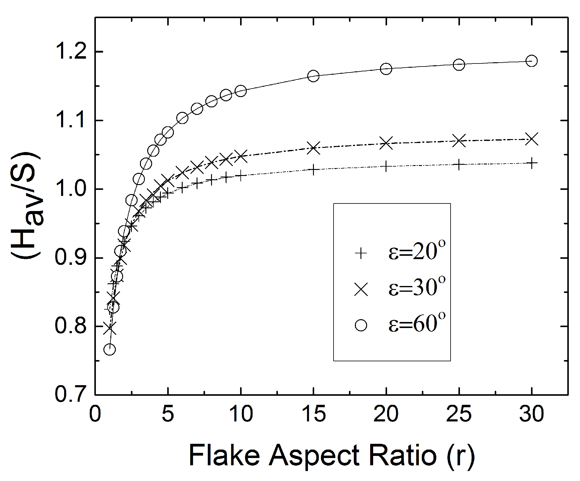
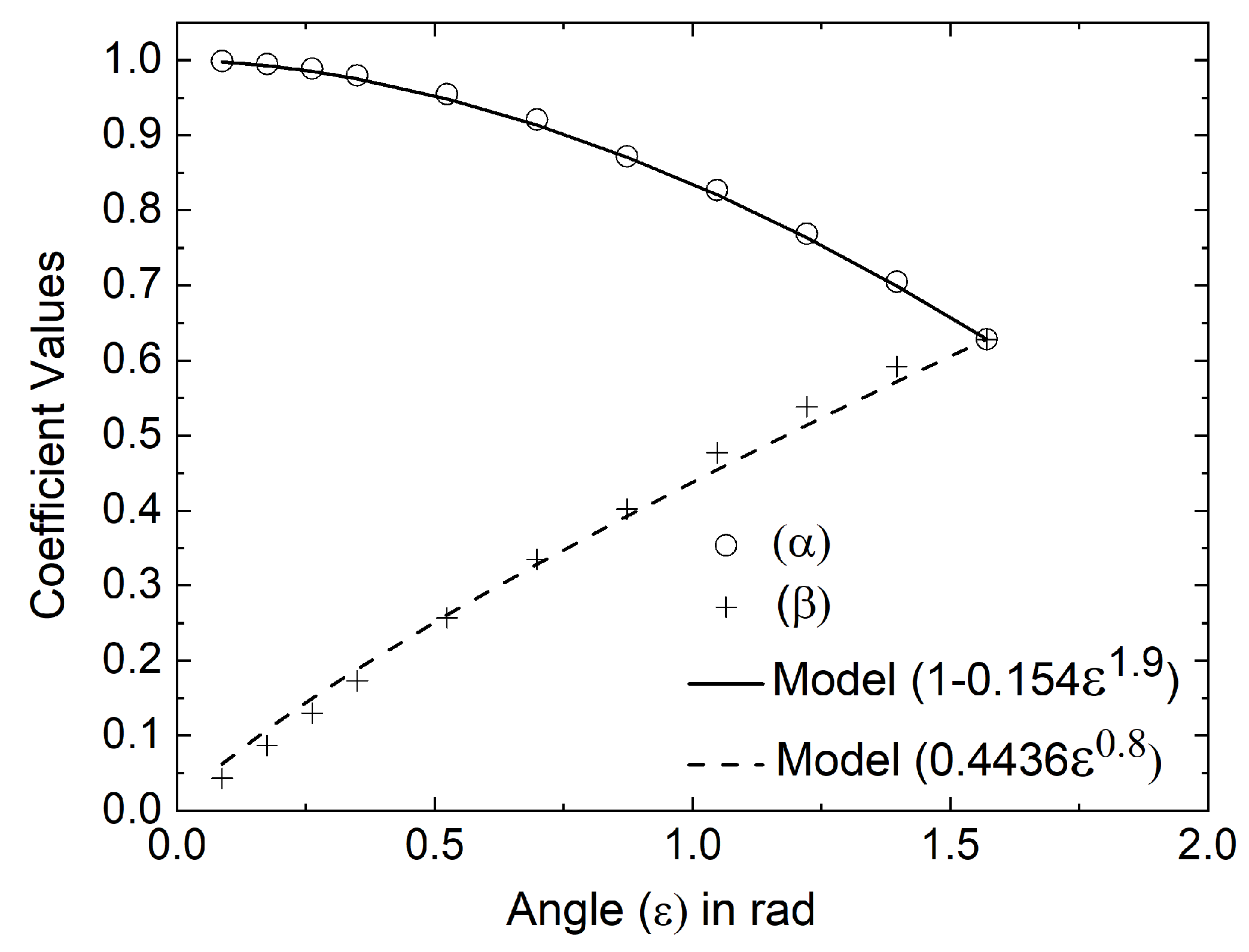
3.2. Estimation of Flake Aspect Ratio and/or Misalignment Angle from the Average Intersection Length

The average intersection length H a v can be computed in a manner similar to the case of flakes having random-in-plane orientations. Figure 7 shows the results for various values of ϵ . It is clear that in this case that H a v is a function of both ϵ and r. We found that a similar functional form describes the dependency of H a v on r, at all levels of ϵ , as was found earlier when ϵ = π / 2 [41]—namely,
H a v S = r α ( ϵ ) r + β ( ϵ )
where the coefficient functions α ( ϵ ) and β ( ϵ ) take the form
α ( ϵ ) = 1 π 2 π 2 π 1.9 ϵ 1.9 = 1 0.1541 ϵ 1.9
β ( ϵ ) = 2 π 1.8 ϵ 0.8 = 0.4436 ϵ 0.8
These fits were designed so that H a v will satisfy the following conditions:
(i)
At ϵ = 0 (flake axis perpendicular to the cutting plane), H a v / S = 1 ;
(ii)
At ϵ = π / 2 (flakes having random in plane orientations), we recover α = β = 2 / π and H a v / S = ( π / 2 ) r / ( r + 1 ) , as found in Ref. [41].
These coefficients are plotted as functions of misalignment angle ϵ in Figure 8.
Equation (10) suggests a scaling by which a master curve can be derived. This is obtained by plotting the average intersection length H a v as H a v α ( ϵ ) r + β ( ϵ ) vs. r, where α ( ϵ ) and β ( ϵ ) are computed from Equations (11) and (12) at each level of the misalignment angle ϵ . The result of this scaling should be a straight line of unit slope. This is shown in Figure 9, in which the results of 900 MC simulations with 0 < ϵ < π / 2 and 1 < r < 21 are plotted, as suggested by Equation (10), for two sample sizes, namely, M = 500 and M = 2000 . The availability of Equation (10) offers the possibility of determining the flake aspect ratio (r) from knowledge of H a v and of the extent of flake misalignment ( ϵ ). In this case, the determination is unambiguous for r < 15 , but progressively deteriorates at higher r, requiring larger sample sizes, in a similar manner as discussed in our previous work for the case of ϵ = π / 2 [41].
Another intriguing possibility offered by Equation (10) is the determination of the extent of misalignment ϵ from knowledge of the average intersection length H a v and of the flake aspect ratio r. To obtain an estimate of ϵ , one has to solve the non-linear algebraic equation of the form of Equation (10), where the coefficient functions α ( ϵ ) and β ( ϵ ) are given by Equations (11) and (12) above. We tested the performance and limits of this approach by numerical sectioning experiments in actual three-dimensional flake systems exhibiting random in-plane flake orientations in the interval [ ϵ , + ϵ ] , such as those shown in Figure 2.
The parity graph of Figure 10 shows the results and the range of ( r , ϵ ) , in which the proposed method can reliably predict the extent of misalignment from knowledge of H a v and r. It is clear that the method is most accurate at larger ϵ values, and for the sample sizes ( M 10 4 ) used in Figure 10, the method is most accurate for ϵ > 35 . Together with the method based on max ( H ) presented earlier (Figure 5), which is most efficient at small ϵ values, these two methods form a complete set of tools that allows the determination of ϵ for the entire range [ π / 2 < ϵ < π / 2 ] and for all flake aspect ratios r > 2 .

4. Conclusions

In this work, we have presented two methods for determining the range of flake misalignment ϵ using the average intersection length H a v and the maximum intersection length max ( H ) . The former is more accurate at larger ϵ , while the latter method, based on max ( H ) , is more accurate at small ϵ . Together, these form a tool set that allows the determination of ϵ for the entire range of π / 2 < ϵ < π / 2 and for all flake aspect ratios r > 2 .
The effect of random in-plane orientation was included in our analysis and results; however, it is not currently possible to deal with flakes having three-dimensional random orientations. This is not a serious limitation, since, due to their planar shape, flakes usually form layered structures with only modest out-of-plane orientations [43].
The focus of our work was on rectangular flakes of all aspect ratios, ranging from squares to thin fiber-like filaments. Our work did not consider poly-disperse systems, such as those that will result when flake attrition is significant. In addition, our work cannot be applied to systems in which the flakes have irregular shapes. Such systems are currently very poorly characterized and more research is needed in this direction.

Author Contributions

Conceptualization and methodology, T.D.P. and A.T.; investigation and analysis, T.D.P., A.T. and Y.W.; writing—original draft preparation, T.D.P. and A.T.; writing—review and editing, T.D.P., A.T. and Y.W. All authors have read and agreed to the published version of the manuscript.

Funding

This research received no external funding.

Data Availability Statement

The raw/processed data required to reproduce these findings cannot be shared at this time as the data also form part of an ongoing study.

Acknowledgments

The authors would like to acknowledge the support of the Greek Research and and Technology Network (GRNET) for the computational time granted in the National HPC facility ARIS. Website: https://hpc.grnet.gr/ (accessed on 27 March 2022).

Conflicts of Interest

The authors declare no conflict of interest.

Abbreviations

The following abbreviations are used in this manuscript:
2Dtwo-dimensional
3Dthree-dimensional
MCMonte-Carlo
RSArandom sequential addition
RVErepresentative volume element

References

  1. Bower, C.M.; Landy, R.A.; Calfee, J.D. Tapes and Ribbons in Composites; Technical Report; Monsato Research Corp: St. Louis, MO, USA, 1965; Available online: https://apps.dtic.mil/sti/citations/AD0488384 (accessed on 27 March 2022).
  2. Padawer, G.E.; Beecher, N. On the Strength and Stiffness of Planar Reinforced Plastic Resins. Polym. Eng. Sci. 1970, 10, 185–192. [Google Scholar] [CrossRef]
  3. Rexer, J.; Anderson, E. Composites with planar reinforcements (flakes, ribbons)—A review. Polym. Eng. Sci. 1979, 19, 1–11. [Google Scholar] [CrossRef]
  4. Thomas, S.; Joseph, K.; Malhotra, S.K.; Goda, K.; Sreekala, M.S. Polymer Composites, Macro-and Microcomposites; John Wiley & Sons: Hoboken, NJ, USA, 2012; Volume 1. [Google Scholar]
  5. Newman, S.; Meyer, F. Mica composites of improved strength. Polym. Compos. 1980, 1, 37–43. [Google Scholar] [CrossRef]
  6. Fenton, M.; Hawley, G. Properties and economics of mica-reinforced plastics related to processing conditions. Polym. Compos. 1982, 3, 218–229. [Google Scholar] [CrossRef]
  7. Bigg, D.M. Mechanical properties of particulate filled polymers. Polym. Compos. 1987, 8, 115–122. [Google Scholar] [CrossRef]
  8. Feng, C.P.; Bai, L.; Bao, R.Y.; Liu, Z.Y.; Yang, M.B.; Chen, J.; Yang, W. Electrically insulating POE/BN elastomeric composites with high through-plane thermal conductivity fabricated by two-roll milling and hot compression. Adv. Compos. Hybrid Mater. 2018, 1, 160–167. [Google Scholar] [CrossRef]
  9. Genetti, W.B.; Yuan, W.L.; Grady, B.P.; O’rear, E.A.; Lai, C.L.; Glatzhofer, D.T. Polymer matrix composites: Conductivity enhancement through polypyrrole coating of nickel flake. J. Mater. Sci. 1998, 33, 3085–3093. [Google Scholar] [CrossRef]
  10. Zhai, S.; Zhang, P.; Xian, Y.; Zeng, J.; Shi, B. Effective thermal conductivity of polymer composites: Theoretical models and simulation models. Int. J. Heat Mass Transf. 2018, 117, 358–374. [Google Scholar] [CrossRef]
  11. Jadhav, N.; Vetter, C.A.; Gelling, V.J. The effect of polymer morphology on the performance of a corrosion inhibiting polypyrrole/aluminum flake composite pigment. Electrochim. Acta 2013, 102, 28–43. [Google Scholar] [CrossRef]
  12. Xia, L.; Wu, H.; Guo, S.; Sun, X.; Liang, W. Enhanced sound insulation and mechanical properties of LDPE/mica composites through multilayered distribution and orientation of the mica. Compos. Part Appl. Sci. Manuf. 2016, 81, 225–233. [Google Scholar] [CrossRef]
  13. Inci, E.; Topcu, G.; Guner, T.; Demirkurt, M.; Demir, M.M. Recent developments of colorimetric mechanical sensors based on polymer composites. J. Mater. Chem. C 2020, 8, 12036–12053. [Google Scholar] [CrossRef]
  14. Xu, M.; Liang, T.; Shi, M.; Chen, H. Graphene-like two-dimensional materials. Chem. Rev. 2013, 113, 3766–3798. [Google Scholar] [CrossRef] [PubMed]
  15. Liu, P.; Cottrill, A.L.; Kozawa, D.; Koman, V.B.; Parviz, D.; Liu, A.T.; Yang, J.; Tran, T.Q.; Wong, M.H.; Wang, S.; et al. Emerging trends in 2D nanotechnology that are redefining our understanding of “Nanocomposites”. Nano Today 2018, 21, 18–40. [Google Scholar] [CrossRef]
  16. Khan, K.; Tareen, A.K.; Aslam, M.; Wang, R.; Zhang, Y.; Mahmood, A.; Ouyang, Z.; Zhang, H.; Guo, Z. Recent developments in emerging two-dimensional materials and their applications. J. Mater. Chem. C 2020, 8, 387–440. [Google Scholar] [CrossRef]
  17. Kilikevičius, S.; Kvietkaitė, S.; Mishnaevsky, L.; Omastová, M.; Aniskevich, A.; Zeleniakienė, D. Novel hybrid polymer composites with graphene and Mxene nano-reinforcements: Computational analysis. Polymers 2021, 13, 1013. [Google Scholar] [CrossRef]
  18. Zhang, Z.; Du, J.; Li, J.; Huang, X.; Kang, T.; Zhang, C.; Wang, S.; Ajao, O.O.; Wang, W.J.; Liu, P. Polymer nanocomposites with aligned two-dimensional materials. Prog. Polym. Sci. 2021, 114, 101360. [Google Scholar] [CrossRef]
  19. Naseem, S.; Wießner, S.; Kühnert, I.; Leuteritz, A. Layered Double Hydroxide (MgFeAl-LDH)-Based Polypropylene (PP) Nanocomposite: Mechanical Properties and Thermal Degradation. Polymers 2021, 13, 3452. [Google Scholar] [CrossRef]
  20. R Manu, B.; Gupta, A.; H Jayatissa, A. Tribological Properties of 2D Materials and Composites—A Review of Recent Advances. Materials 2021, 14, 1630. [Google Scholar] [CrossRef]
  21. Rana, S.; Singh, V.; Singh, B. Recent trends in 2D materials and their polymer composites for effectively harnessing mechanical energy. iScience 2022, 103748. [Google Scholar] [CrossRef]
  22. Yang, C.; Smyrl, W.H.; Cussler, E.L. Flake alignment in composite coatings. J. Membr. Sci. 2004, 231, 1–12. [Google Scholar] [CrossRef]
  23. Idris, A.; Muntean, A.; Mesic, B. A review on predictive tortuosity models for composite films in gas barrier applications. J. Coat. Technol. Res. 2022, 1–18. [Google Scholar] [CrossRef]
  24. Zid, S.; Zinet, M.; Espuche, E. Modeling diffusion mass transport in multiphase polymer systems for gas barrier applications: A review. J. Polym. Sci. B Polym. Phys. 2018, 56, 621–639. [Google Scholar] [CrossRef] [Green Version]
  25. Boldt, R.; Leuteritz, A.; Schob, D.; Ziegenhorn, M.; Wagenknecht, U. Barrier Properties of GnP–PA-Extruded Films. Polymers 2020, 12, 669. [Google Scholar] [CrossRef] [PubMed] [Green Version]
  26. Gaska, K.; Kádár, R.; Rybak, A.; Siwek, A.; Gubanski, S. Gas barrier, thermal, mechanical and rheological properties of highly aligned graphene-LDPE nanocomposites. Polymers 2017, 9, 294. [Google Scholar] [CrossRef] [PubMed]
  27. Chen, X.; Papathanasiou, T.D. Barrier properties of flake-filled membranes: Review and numerical evaluation. J. Plast. Film. Sheeting 2007, 23, 319–346. [Google Scholar] [CrossRef]
  28. Tsiantis, A.; Papathanasiou, T.D. A general scaling for the barrier factor of composites containing thin layered flakes of rectangular, circular and hexagonal shape. Int. J. Heat Mass Transf. 2020, 157, 119962. [Google Scholar] [CrossRef]
  29. Tsiantis, A.; Wang, Y.; Huang, X.; Papathanasiou, T.D. From flakes to ribbons: The barrier factor of composites containing flakes of rectangular shape. J. Compos. Mater. 2022, 56, 181–198. [Google Scholar] [CrossRef]
  30. Decker, J.J.; Meyers, K.P.; Paul, D.R.; Schiraldi, D.A.; Hiltner, A.; Nazarenko, S. Polyethylene-based nanocomposites containing organoclay: A new approach to enhance gas barrier via multilayer coextrusion and interdiffusion. Polymer 2015, 61, 42–54. [Google Scholar] [CrossRef]
  31. Spencer, M.W.; Hunter, D.L.; Knesek, B.W.; Paul, D.R. Morphology and properties of polypropylene nanocomposites based on a silanized organoclay. Polymer 2011, 52, 5369–5377. [Google Scholar] [CrossRef]
  32. Zhang, D.; Zhan, Z. Strengthening effect of graphene derivatives in copper matrix composites. J. Alloys Compd. 2016, 654, 226–233. [Google Scholar] [CrossRef]
  33. Adak, B.; Joshi, M.; Butola, B.S. Polyurethane/clay nanocomposites with improved helium gas barrier and mechanical properties: Direct versus master-batch melt mixing route. J. Appl. Polym. Sci. 2018, 135, 46422. [Google Scholar] [CrossRef]
  34. Clarke, A.; Davidson, N.; Archenhold, G. Mesostructural characterisation of aligned fibre composites. In Flow-Induced Alignment in Composite Materials; Papathanasiou, T.D., Bénard, A., Eds.; Elsevier: Amsterdam, The Netherlands, 1997; pp. 230–292. [Google Scholar]
  35. Da Costa, J.P.; Oprean, S.; Baylou, P.; Germain, C. Stereological estimation of orientation distribution of generalized cylinders from a unique 2D slice. Microsc. Microanal. 2013, 19, 1678–1687. [Google Scholar] [CrossRef] [PubMed] [Green Version]
  36. Clarke, A.; Eberhardt, C. The representation of reinforcing fibres in composites as 3D space curves. Compos. Sci. Technol. 1999, 59, 1227–1237. [Google Scholar] [CrossRef]
  37. Eberhardt, C.; Clarke, A.; Vincent, M.; Giroud, T.; Flouret, S. Fibre-orientation measurements in short-glass-fibre composites—II: A quantitative error estimate of the 2d image analysis technique. Compos. Sci. Technol. 2001, 61, 1961–1974. [Google Scholar] [CrossRef]
  38. Bale, H.; Blacklock, M.; Begley, M.R.; Marshall, D.B.; Cox, B.N.; Ritchie, R.O. Characterizing three-dimensional textile ceramic composites using synchrotron X-ray micro-computed-tomography. J. Am. Ceram. Soc. 2012, 95, 392–402. [Google Scholar] [CrossRef]
  39. Lee, Y.; Lee, S.; Youn, J.; Chung, K.; Kang, T. Characterization of fiber orientation in short fiber reinforced composites with an image processing technique. Mater. Res. Innov. 2002, 6, 65–72. [Google Scholar] [CrossRef]
  40. Martín-Herrero, J.; Germain, C. Microstructure reconstruction of fibrous C/C composites from X-ray microtomography. Carbon 2007, 45, 1242–1253. [Google Scholar] [CrossRef] [Green Version]
  41. Papathanasiou, T.D.; Tsiantis, A.; Wang, Y. A Novel Method for the Determination of the Lateral Dimensions of 2D Rectangular Flakes. Materials 2022, 15, 1560. [Google Scholar] [CrossRef]
  42. Tsiantis, A.; Papathanasiou, T.D. A novel FastRSA algorithm: Statistical properties and evolution of microstructure. Phys. Stat. Mech. Its Appl. 2019, 534, 122083. [Google Scholar] [CrossRef]
  43. Papathanasiou, T.D.; Bénard, A. (Eds.) Flow-Induced Alignment in Composite Materials; Woodhead Publishing: Cambridge, UK, 2021. [Google Scholar]
  44. Barwick, S.C.; Papathanasiou, T.D. Identification of fiber misalignment in continuous fiber composites. Polym. Compos. 2003, 24, 475–486. [Google Scholar] [CrossRef]
Figure 1. Top view of sample geometries showing flakes oriented at different intervals [ ϵ , + ϵ ] around the y-axis. (a) ϵ = 15 , (b) ϵ = 45 . In both images the aspect ratio r = 3 . For visual clarity, only a few flakes are shown. In the sectioning experiments used to validate the results of this work, each composite contained up to 10 6 individual flakes.
Jcs 06 00142 g001
Figure 2. Schematic showing a numerical sectioning experiment. (a) 3D RVE containing flakes with their planes parallel to the X-Z plane and having random orientations in the X-Y plane. Shown as well are the sectioning planes. (b) The sectioning planes showing only the flake intersections as lines of variable length. The number of sections defines the ensemble size (here K = 4 ). The number of intersections (lines) in each frame, defines the sample size (here M 50 for clarity). Reprinted from Papathanasiou et al. [41].
Jcs 06 00142 g002
Figure 3. Basic geometrical features of the problem. The intersection between the cutting plane and the plane of the flake (line (c) in the schematic) will be tangent to a circle of radius L, centered at the center of the flake. The counter-clockwise angle formed between the long axis of the rectangle and line c is π / 2 + θ . Thus, θ = 0 corresponds to line (c) being perpendicular to the long axis of the rectangle, and, when θ = π / 2 , line (c) is parallel to the long axis of the rectangle. Reprinted from Papathanasiou et al. [41].
Jcs 06 00142 g003
Figure 4. (a) Histograms of intersection lengths, normalized by dividing with the short side (S) of the rectangle, for flakes of aspect ratio r = 2 and three levels of ϵ values and (b) constant ϵ = π / 6 and three values of r. In each case, the number of bins is 100. The logarithmic axis is used for the frequency of intersection lengths, since, when ϵ is small, the overwhelming majority of intersection lengths are S ; very few intersections have lengths less or greater than S. It is obvious that the peak occurs at H / S = 1 and also that there is no secondary peak when ϵ < π / 2 . In each case, 2 × 10 5 random pairs of (L, θ ) were used in obtaining the histograms. It is also clear from (b) that max ( H ) is independent of r, and from (a) it is evident that max ( H ) is a function of ϵ .
Jcs 06 00142 g004
Figure 5. (a) Results of MC simulations, illustrating a correlation between max ( H ) and ϵ (in degrees), obtained for 2 < r < 20 , and for various sample sizes M. The correlation is valid for any r 2 and 0 < ϵ < 60 and for sample size M 10 3 . (b) Parity graph between the actual misalignment angle ϵ and the value of ϵ e s t computed from Equation (6).
Jcs 06 00142 g005
Figure 6. The probability of achieving intersection lengths that satisfy Equation (7) at the 1 % level ( h = 0.01 ), as a function of the misalignment angle ϵ . Lines show the predictions of Equation (9) for two values of r. Points are results of MC simulations, using 2 × 10 5 random pairs of (L, θ ) and 5 repetitions at each level of r and ϵ . Since it must be cos ϵ / ( 1 h ) < 1 in Equation (9), it follows that for h = 0.01 that allowable values of ϵ are ϵ > 8 . 1 . The vertical arrow next to the column of the MC data at ϵ = 60 indicates the direction of increasing the aspect ratio r ( 2 < r < 20 ).
Jcs 06 00142 g006
Figure 7. Comparison between the average intersection length H a v / S predicted from Equation (10) (lines) and values computed from numerical sectioning experiments (points) for various values of ϵ and r.
Jcs 06 00142 g007
Figure 8. Dependence of the coefficients α and β of Equation (10) on ϵ and the model fits suggested by Equations (11) and (12).
Jcs 06 00142 g008
Figure 9. Computational results for H a v , plotted as suggested by Equation (10). Each data point was obtained from one sample having M flake intersections with flakes of aspect ratio r and random orientation in the interval [– ϵ , + ϵ ], 0 < ϵ < π / 2 . While the scatter around the line of unit slope is slightly higher at larger values of r and for a smaller sample size M, the best fit lines through all data have slopes that are very close to 1.
Jcs 06 00142 g009
Figure 10. Parity graph between misalignment angle in the actual sample (in degrees, horizontal axis) and the back-calculated ϵ obtained by solving Equation (10) in which H a v and r are known (vertical axis). Data points indicate results from samples at various values of r, as indicated, and for the ϵ corresponding to the horizontal axis. Data points falling close to the line of slope one (shown) indicate reliable algorithm predictions. In all cases, sample size M 10 4 .
Jcs 06 00142 g010
Publisher’s Note: MDPI stays neutral with regard to jurisdictional claims in published maps and institutional affiliations.

