High-Dimensional LASSO-Based Computational Regression Models: Regularization, Shrinkage, and Selection

Abstract

Regression models are a form of supervised learning methods that are important for machine learning, statistics, and general data science. Despite the fact that classical ordinary least squares (OLS) regression models have been known for a long time, in recent years there are many new developments that extend this model significantly. Above all, the least absolute shrinkage and selection operator (LASSO) model gained considerable interest. In this paper, we review general regression models with a focus on the LASSO and extensions thereof, including the adaptive LASSO, elastic net, and group LASSO. We discuss the regularization terms responsible for inducing coefficient shrinkage and variable selection leading to improved performance metrics of these regression models. This makes these modern, computational regression models valuable tools for analyzing high-dimensional problems.

1. Introduction

The increasing digitalization of our society and progress in the development of new measurement devices has led to a flood of data. For instance, data from social media enable the development of methods for their analysis to address relevant questions in the computational social sciences [1,2]. In biology or the biomedical sciences, novel sequencing technologies enable the generation of high-throughput data from all molecular levels, including mRNAs, proteins, and DNA sequences [3,4]. Depending on the characteristics of the data, appropriate analysis methods need to be selected for their interrogations. One of the most widely used analysis methods is regression models [5,6]. Put simply, this type of method performs a mapping from a set of input variables to output variables. In contrast to classification methods, the output variables for regression models assume real values. Due to the fact that many application problems come in this form, regression models find widespread applications across many fields, e.g., [7,8,9,10,11].

In recent years, several new regression models have been introduced that extend classical regression models significantly. The purpose of this paper is to review such regression models, with a special focus on the least absolute shrinkage and selection operator (LASSO) model [12] and extensions thereof. Specifically, in addition to the LASSO, we will discuss the non-negative garrotte [13], Dantzig selector [14], Bridge regression [15], adaptive LASSO [16], elastic net [17], and group LASSO [18].

Interestingly, despite the popularity of the LASSO, there are only very few reviews available about this model. In contrast to previous reviews about this topic [9,19,20,21], our focus is different with respect to the following points. First, we focus on the LASSO and advanced models related to the LASSO. Our aim is not to cover all regression models but regularized regression models centered around the LASSO (the concept of regularization has been introduced by Tikhonov to approximate ill-posed inverse problems [22,23]). Second, we present the necessary technical details of the methods to the level where they are needed for a deeper understanding. However, we do not present all details especially if they are related to the proof of properties. Third, our explanations aim at an intermediate level of the reader by providing also background information frequently omitted in advanced texts. This should ensure that our review is useful for a broad readership from many areas. Fourth, we use a data set from economics to discuss properties of the methods and to cross-discuss differences among them. Fifth, we will provide information about the practical application of the methods by providing information about availability of implementations for the statistical programming language R. In general, there are many software packages available in different implementations and programming languages but we focus on R because the more statistics oriented literature favors this programming language.

This paper is organized as follows. In the next section, we present general preprocessing steps we use before a regression analysis and we discuss an example data set we use to demonstrate the different models. Thereafter, we discuss ordinary least squares regression and ridge regression because we assume that not all readers will be familiar with these models but an understanding of these is necessary in order to understand more advanced regression models. Then we discuss the non-negative garrotte, LASSO, Bridge regression, Dantzig selector, adaptive LASSO, elastic net, and group LASSO, with a special focus on the regularization term. The paper finishes with a brief summary of the methods and conclusions.

2. Preprocessing of Data and Example Data

We begin our paper by briefly providing some statistical preliminaries needed for the regression models. First, we discuss some preprocessing steps used for standardizing the data for all regression models. Second, we discuss data we are using to demonstrate the differences of the different regression models.

2.1. Preprocessing

Let us assume we have data of the form $({\mathit{x}}_i,y_i)$ with $i\in \{1,\dots ,n\}$, where n is the number of samples. The vector ${\mathit{x}}_i$ corresponds to the predictor variables for sample i, whereas ${\mathit{x}}_i={(X_{i1},\dots ,X_{ip})}^T$ and p is the number of predictors, furthermore $y_i$ is the response variable. We denote by $\mathit{y}\in {\mathbb{R}}^n$ the vector of response variables and by $\mathit{X}\in {\mathbb{R}}^{n\times p}$ the predictor matrix. The vector $\mathit{\beta }={({\beta }_1,\dots ,{\beta }_p)}^T$ gives the regression coefficients.

The predictors and response variable shall be standardized, which means:

$$\begin{array}{ccc}\hfill {\overline{x}}_j& =& \frac{1}{n}\sum _{i=1}^n{X}_{ij}=0\mathrm{for}\mathrm{all}j\hfill \end{array}$$

(1)

$$\begin{array}{ccc}\hfill {\overline{s}}_j^2& =& \frac{1}{n}\sum _{i=1}^n{X}_{ij}^2=1\mathrm{for}\mathrm{all}j\hfill \end{array}$$

(2)

$$\begin{array}{ccc}\hfill \overline{y}& =& \frac{1}{n}\sum _{i=1}^n{y}_i=0\hspace{1em}\hspace{1em}\hspace{1em}\hspace{1em}\hfill \end{array}$$

(3)

Here ${\overline{x}}_j$ and ${\overline{s}}_j^2$ are the mean and variance of the predictor variables and $\overline{y}$ is the mean of the response variables.

In order to study the regularization of regression models, we need to solve optimization problems which are formulated in terms of norms. For this reason, we review in the following the norms needed for the subsequent sections. For a real vector $\mathit{x}\in {\mathbb{R}}^n$ and $q\ge 1$ the Lq-norm is defined by

$$\begin{array}{c}\hfill {\parallel \mathit{x}\parallel }_q={\left(\sum _{i=1}^n{\left|x_i\right|}^q\right)}^{\frac{1}{q}}.\end{array}$$

(4)

For the special case $q=2$ one obtains the L2-norm (also known as Euclidean norm) and for $q=1$ the L1-norm. Interestingly, for $q<1$ Equation (4) is defined but no longer a norm in the mathematical sense.

We will revisit the L2-norm when discussion ridge regression and the L1-norm for the LASSO. The infinity norm, also called maximum norm, is defined by

$$\begin{array}{c}\hfill {\parallel \mathit{x}\parallel }_{\infty }=\underset{i}{max}\left|x_i\right|.\end{array}$$

(5)

This norm is used by the Danzig selector.

For $q=0$ one obtains the L0-norm which corresponds to the number of non-zero elements, i.e.,

$$\begin{array}{c}\hfill {\parallel \mathit{x}\parallel }_0=\#\mathrm{non}-\mathrm{zero}\mathrm{elements}.\end{array}$$

(6)

2.2. Data

In order to provide some practical examples for the regression models, we use a data set from [24]. The whole data set consists of 156 samples for 93 economic variables about inflation indexes and macroeconomic variables of the Brazilian econnomy. From these we select 7 variables to predict the Brazilian inflation. We focus on 7 variables because these are sufficient to demonstrate the regularization, shrinkage, and selection of the different regression models we discuss in the following sections. Using more variables leads quickly to cumbersome models that require much more effort for their understanding without providing more insights regarding the focus of our paper.

3. Ordinary Least Squares Regression

We begin our discussion by formulating a multiple regression problem,

$$\begin{array}{c}\hfill y_i=\sum _{j=1}^p{X}_{ij}{\beta }_j+{ϵ}_i.\end{array}$$

(7)

Here $X_{ij}$ are p predictor variables that are linearly mapped onto the response variable $y_i$ for sample i. The mapping is defined by the p regression coefficients ${\beta }_j$. Furthermore, the mapping is effected by a noise term ${ϵ}_i$ assuming values in $\sim N(0,{\sigma }^2)$. The noise term summarizes all kinds of uncertainties, e.g., measurement errors.

In order to see the similarity between a multiple linear regression, having p predictor variables, and a simple linear regression, having one predictor variable, one can write Equation (7) in the form:

$$\begin{array}{c}\hfill y_i={\mathit{x}}_i^T\mathit{\beta }+{ϵ}_i\end{array}$$

(8)

Here ${\mathit{x}}_i^T\mathit{\beta }$ is the inner product (scalar product) between the two p-dimensional vectors ${\mathit{x}}_i={(X_{i1},\dots ,X_{ip})}^T$ and $\mathit{\beta }={({\beta }_1,\dots ,{\beta }_p)}^T$. One can further summarize Equation (8) for all samples $i\in \{1,\dots ,n\}$ by

$$\begin{array}{c}\hfill \mathit{y}=\mathit{X}\mathit{\beta }+ϵ.\end{array}$$

(9)

Here the noise terms assumes the form $ϵ\sim N(0,{\sigma }^2{\mathit{I}}_n)$ whereas ${\mathit{I}}_n$ is the ${\mathbb{R}}^{n\times n}$ identity matrix.

The solution of Equation (9) can be formulated as an optimization problem given by

$$\begin{array}{c}\hfill {\widehat{\mathit{\beta }}}^{OLS}=argmin{\parallel \mathit{y}-\mathit{X}\mathit{\beta }\parallel }_2^2.\end{array}$$

(10)

The ordinary least squares (OLS) solution of Equation (10) can be analytically calculated assuming X has full column rank, which implies that $X^{T}X$ is positive definite, and is given by

$$\begin{array}{c}\hfill {\widehat{\mathit{\beta }}}^{OLS}={\left({\mathit{X}}^T\mathit{X}\right)}^{-1}{\mathit{X}}^T\mathit{y}.\end{array}$$

(11)

If X has not full column rank the solution cannot be uniquely determined.

Limitations

Least squares regression can perform very badly when there are outliers in the data. For this reason it can be very helpful in performing outlier detection in the data before the analysis is performed and removing the outliers from the data before applying it to the regression model. A reason why least squares regression is so sensitive to outliers is that this model does not perform any form of coefficient shrinkage of regression coefficients as, e.g., the LASSO. For this reasons coefficients can become very large as a result of such outliers without a limiting mechanism built into the model.

Another factor that can lead to a bad performance is the correlation between predictor variables. The disadvantage of the regression model is that it does not perform any form of variable selection to reduce the numbers of predictor variables as, e.g., ridge regression or LASSO. Instead, it uses the variables specified as input to the model.

The third factor that can reduce the performance is called heteroskedasticity or heteroscedasticity. It refers to varying (non-constant) variances of the error term in dependence on the sampling region. One particular problem caused by heteroskedasticity is that it leads to inefficient and biased estimates of the OLS standard errors and, hence, results in biased statistical tests of the regression coefficients [25].

In summary, ordinary least squares regression neither performs shrinkage nor variable selection, which can lead to problems as discussed above. For this reason, advanced regression models have been introduced to guard against such problems.

4. Ridge Regression

The motivation for improving OLS is the fact that the estimates from such models have often a low bias but a large variance. This is related to the prediction accuracy of a model because it is known that either by shrinking the values of regression coefficients or by setting coefficients to zero the accuracy of a prediction can be improved [26]. The reason for this is that by introducing some estimation bias the variance can be actually reduced.

Ridge regression has been introduced by [27]. The model can be formulated as follows.

$$\begin{array}{ccc}\hfill {\widehat{\mathit{\beta }}}^{RR}& =& argmin\left\{\frac{1}{2n}\sum _{i=1}^n{(y_i-\sum _j{x}_{ij}{\beta }_j)}^2+\lambda {\parallel \mathit{\beta }\parallel }_2^2\right\}\hfill \end{array}$$

(12)

$$\begin{array}{cc}=& argmin\left\{\frac{1}{2n}\mathrm{RSS}\left(\mathit{\beta }\right)+\lambda {\parallel \mathit{\beta }\parallel }_2^2\right\}\hspace{1em}\hspace{1em}\hspace{1em}\hfill \end{array}$$

(13)

$$\begin{array}{cc}=& argmin\{\frac{1}{2n}\parallel {\mathit{y}-\mathit{X}\mathit{\beta }\parallel }_2^2+\lambda {\parallel \mathit{\beta }\parallel }_2^2\}\hspace{1em}\hfill \end{array}$$

(14)

Here $\mathrm{RSS}\left(\mathit{\beta }\right)$ is the residual sum of squares (RSS) called the loss of the model, ${\lambda \parallel \mathit{\beta }\parallel }_2^2$ is the regularization term or penaltyd, and $\lambda$ is the tuning or regularization parameter. The parameter $\lambda$ controls the shrinkage of coefficients. The L2-penalty in Equation (12) is sometimes also called Tikhonov regularization.

Ridge regression has an analytical solution which is given by

$$\begin{array}{c}\hfill {\widehat{\mathit{\beta }}}^{RR}\left(\lambda \right)={\left({\mathit{X}}^T\mathit{X}+\lambda {\mathit{I}}_p\right)}^{-1}{\mathit{X}}^T\mathit{y}.\end{array}$$

(15)

Here ${\mathit{I}}_p$ is the $p\times p$ identity matrix. A problem of OLS is that if $rank\left(\mathit{X}\right)<p$, then ${\mathit{X}}^T\mathit{X}$ does not have an inverse. However, a non-zero regularization parameter $\lambda$ leads usually to a matrix ${\mathit{X}}^T\mathit{X}+\lambda {\mathit{I}}_p$, for which an inverse exists.

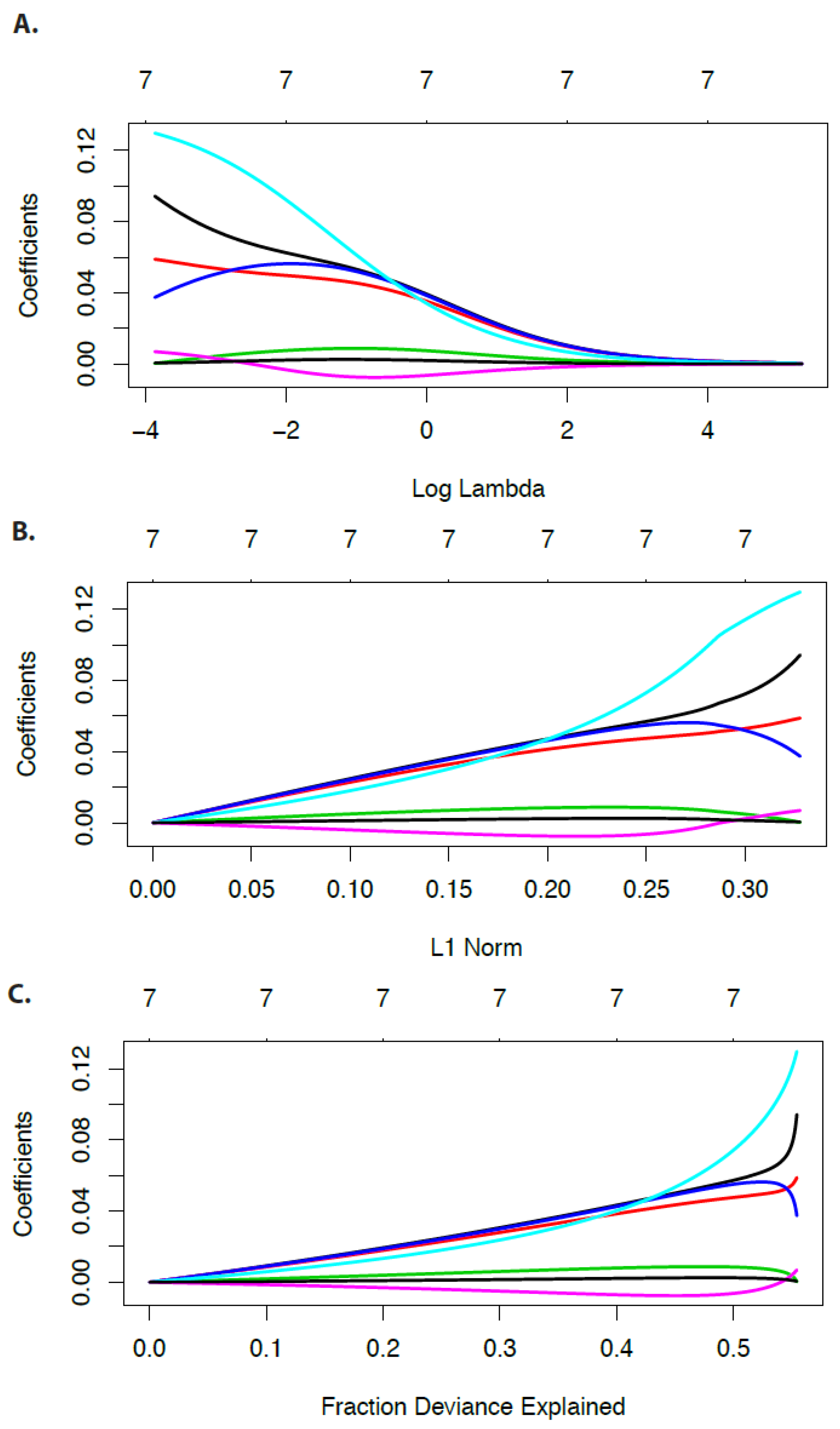
In Figure 1, we show numerical examples for the economic data set. Specifically, in Figure 1A–C we show the regression coefficients in dependence on $\lambda$ because the solution in Equation (15) depends on the tuning parameter. On the top of each figure the numbers of non-zero regression coefficients are shown. One can see that for decreasing value of $\lambda$ the values of the regression coefficients are decreasing. This is the shrinkage effect of the tuning parameter. Furthermore, one can see that none of the coefficients becomes zero. Instead, all regression coefficients assume small but non-zero values. These observations are characteristics for general results from ridge regression [26].

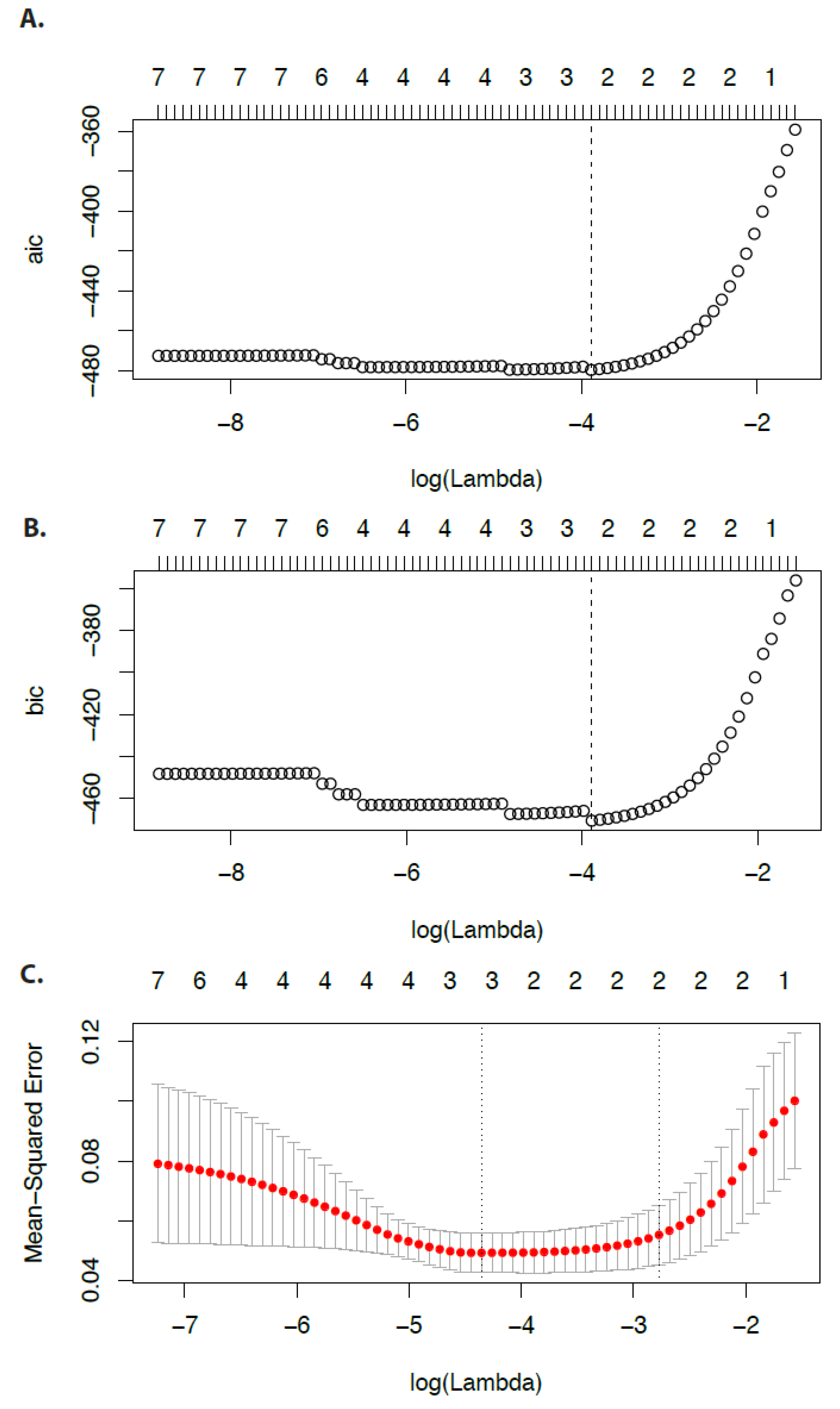
In Figure 2, we show results for the Akaike information criterion (AIC) (Figure 2A), the Bayesian information criterion (BIC) (Figure 2B), and the mean-squared error (Figure 2C). Again, the numbers on top of the figures give the number of non-zero regression coefficients. Each criterion can be used to identify an optimal $\lambda$ value (see the vertical dashed lines). However, using AIC or BIC would lead to $\lambda$ values that do not perform a shrinkage of the coefficients (see Figure 1A). In contrast, the mean-squared error suggests a smaller value of the tuning parameter that indeed shrinks the coefficients.

Overall, the advantages of a ridge regression is that it can reduce the variance by paying the price of an increasing bias. This can improve the prediction accuracy of a model. This works best in situations where the OLS estimates have a high variance and for the cases $p<n$.

A disadvantage is that ridge regression does not shrink coefficient to zero and, hence, does not perform variable selection. Another motivating factor for improving upon OLS is that by reducing the number of predictors the interpretation of a model becomes easier because one can focus on the relevant variables of the problem.

R Package

Ridge regression can be performed using the glmnet R package [28]. This package is flexible allowing to perform also other types of regularized regression models (see LASSO and adaptive LASSO).

5. Non-Negative Garotte Regression

The next model we discuss, the non-negative garotte, has been mentioned as a motivation for the introduction of the LASSO [12]. For this reason we discuss it before the LASSO. The non-negative garotte has been introduced by [13] and is given by

$$\begin{array}{ccc}\hfill \widehat{\beta }& =& argmin\{\frac{1}{2n}\parallel {\mathit{y}-\mathit{Z}\mathit{d}\parallel }_2^2+\lambda \sum _{j=1}^p{d}_j\},\hfill \end{array}$$

(16)

for $\mathit{d}={(d_1,\dots ,d_p)}^T$ with $d_j>0$ for all j. The regression is formulated for the scaled variables $\mathit{Z}$ given by $Z_j=X_j{\widehat{\beta }}_j^{OLS}$. That means the model, first, estimates ordinary least squares parameter ${\widehat{\beta }}_j^{OLS}$ for the unregularized regression (Equation (10)) and then performs in a second step a regularized regression for the scaled predictors $\mathit{Z}$.

The non-negative garotte estimate can be expressed with the OLS regression coefficient and the regularization coefficients by [29]

$$\begin{array}{c}\hfill {\widehat{\beta }}_j^{NNG}\left(\lambda \right)=d_j\left(\lambda \right){\widehat{\beta }}_j^{OLS}.\end{array}$$

(17)

Breiman showed that the non-negative garotte has consistently lower prediction error than subset selection and is competitive with ridge regression except when the true model has many small non-zero coefficients. A disadvantage of the non-negative garotte is its explicit dependency on the OLS estimates [12].

6. LASSO

The LASSO (least absolute shrinkage and selection operator) has been made popular by Robert Tibshirani in 1996 [12], but it had previously appeared in the literature see, e.g., [30,31]. It is a regression analysis method that performs both variable selection and regularization in order to enhance the prediction accuracy and interpretability of the statistical regression model.

The LASSO estimate of $\widehat{\beta }$ is given by:

$$\begin{array}{c}\hfill \widehat{\mathit{\beta }}=argmin\left\{\frac{1}{2n}\sum _{i=1}^n{(y_i-\sum _j{\beta }_j{x}_{ij})}^2\right\}\end{array}$$

(18)

$$\begin{array}{c}\hfill {\mathrm{subject}\mathrm{to}:\parallel \mathit{\beta }\parallel }_1\le t\end{array}$$

(19)

Equation (18) is called the constrained form of the regression model. In Equation (19) t is a tuning parameter (also called regularization parameter or penalty parameter) and ${\parallel \mathit{\beta }\parallel }_1$ the L1-norm (see Equation (4)).

It can be shown that Equation (18) can be written in the Lagrange form given by:

$$\begin{array}{ccc}\hfill \widehat{\mathit{\beta }}& =& argmin\left\{\frac{1}{2n}\sum _{i=1}^n{(y_i-\sum _j{\beta }_j{x}_{ij})}^2+\lambda {\parallel \mathit{\beta }\parallel }_1\right\}\hfill \end{array}$$

(20)

$$\begin{array}{cc}=& argmin\{\frac{1}{2n}\parallel {\mathit{y}-\mathit{X}\beta \parallel }_2^2+\lambda {\parallel \mathit{\beta }\parallel }_1\}\hspace{1em}\hspace{1em}\hfill \end{array}$$

(21)

The relation between both forms holds due to the duality and the KKT (Karush-Kuhn-Tucker) conditions. Furthermore, for every $t>0$ there exists a $\lambda >0$ such that both equations lead to the same solution [26].

In general, the LASSO lacks a closed form solution because the objective function is not differentiable. However, it is possible to obtain closed form solutions for the special case of an orthonormal design matrix.

In the LASSO regression model Equation (21), $\lambda$ is a parameter that needs to be estimated. This is accomplished by cross-validation. Specifically, for each fold $F_k$ the mean-squared error is estimated by

$$\begin{array}{c}\hfill e{\left(\lambda \right)}_k=\frac{1}{\#F_k}\sum _{j\in F_k}{(y_j-{\widehat{y}}_j)}^2.\end{array}$$

(22)

Here $\#F_k$ is the number of samples in set $F_k$. Then the average over all K folds is taken,

$$\begin{array}{c}\hfill CV\left(\lambda \right)=\frac{1}{K}\sum _{k=1}^{K}e{\left(\lambda \right)}_k.\end{array}$$

(23)

This is called the cross-validation mean-squared error. For obtaining an optimal $\lambda$ from $CV\left(\lambda \right)$, two approaches are common. The first estimates the $\lambda$ that minimizes the function $CV\left(\lambda \right)$,

$$\begin{array}{c}\hfill {\widehat{\lambda }}_{min}=argminCV\left(\lambda \right).\end{array}$$

(24)

The second approach, first, estimates ${\widehat{\lambda }}_{min}$ and then identifies the maximal $\lambda$ that has a cross-validation MSE (mean squared error) smaller than $CV\left({\widehat{\lambda }}_{min}\right)+SE\left({\widehat{\lambda }}_{min}\right)$, given by

$$\begin{array}{c}\hfill {\widehat{\lambda }}_{1se}=\underset{CV\left(\lambda \right)\le CV\left({\widehat{\lambda }}_{min}\right)+SE\left({\widehat{\lambda }}_{min}\right)}{max}\lambda .\end{array}$$

(25)

6.1. Example

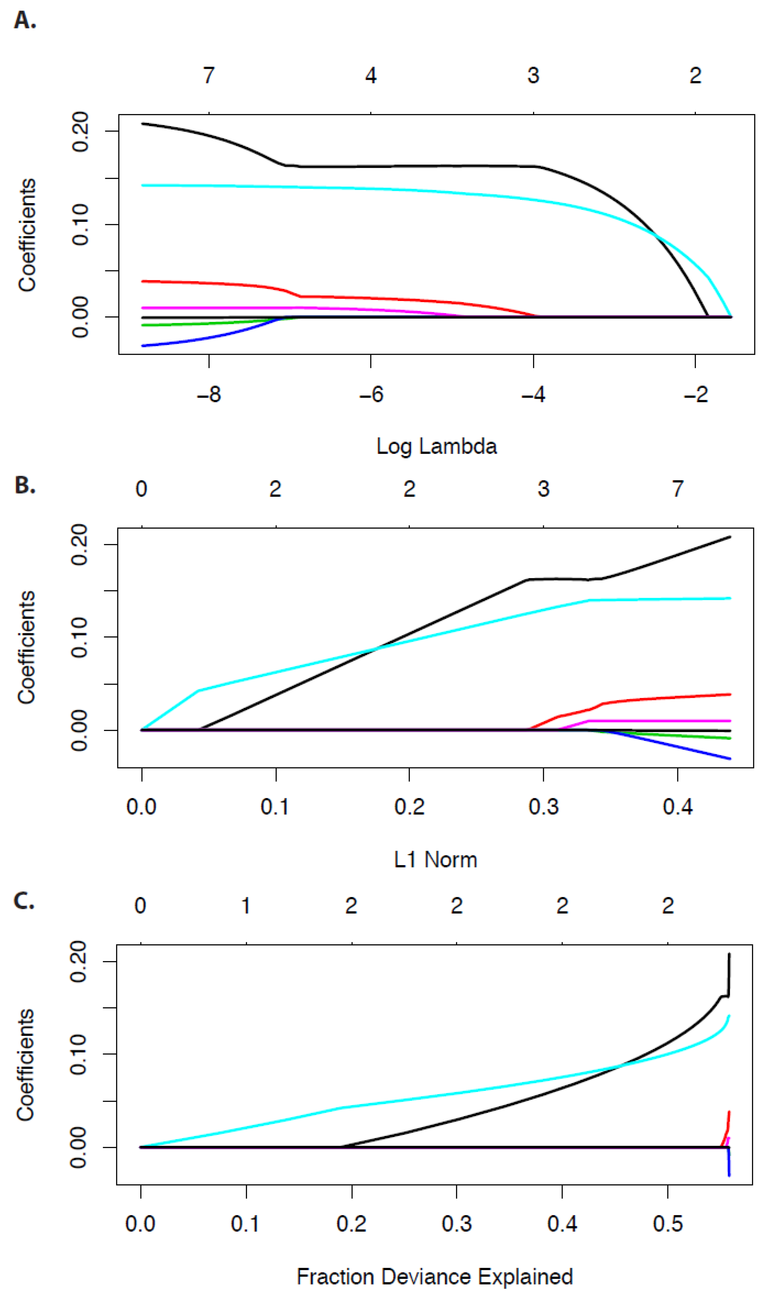
In Figure 3 and Figure 4 we show examples for the economy data. In Figure 3 we show coefficient paths for the LASSO regression model in dependence on $log\left(\lambda \right)$ (A), the L1-norm (B), and the fraction of deviance explained (C).

In Figure 4 we show the Akaike information criterion, the Bayesian information criterion (see [32]), and the Mean-squared error of $\lambda$.

6.2. Explanation of Variable Selection

From Figure 3 one can see that decreasing values of $\lambda$ lead to the shrinkage of the regression coefficients and some of these even become zero. To understand this behavior, we depict in Figure 5A,B a two-dimensional LASSO (A) and ridge regression (B) model. The regularization term of each regression model is depicted in blue, corresponding to the diamond shape for the L1-norm and the circle for the L2-norm. The solution of the optimization problem is given by the intersection of the ellipsis and the boundary of the penalty shapes. These intersections are highlighted by a green point for the LASSO and a blue point for the ridge regression. In order to shrink a coefficient to zero an intersection needs to occur alongside the two coordinate axis. For the shown situation this is only possible for the LASSO but not for ridge regression. In general, the probability for a LASSO to shrink a coefficient to zero is much larger than for the ridge regression.

In order to understand this, it is helpful to look at the solution for the coefficients for the orthonormal case, because for this situation, the solution for the LASSO can be found analytically. The analytical solution is given by

$$\begin{array}{c}\hfill {\widehat{\beta }}_i^{LASSO}(\lambda ;orth)=\mathrm{sign}\left(\widehat{{\beta }_i^{OLS}}\right)S(\widehat{{\beta }_i^{OLS}},\lambda ).\end{array}$$

(26)

Here $S\left(\right)$ is the soft-threshold operator defined as:

$$\begin{array}{c}\hfill S(\widehat{{\beta }_i^{OLS}},\lambda )=\left\{\begin{array}{cc}\widehat{{\beta }_i^{OLS}}-\lambda \phantom{\infty }\hfill & \mathrm{if}\widehat{{\beta }_i^{OLS}}>\lambda \hfill \\ 0\phantom{0}\hfill & \mathrm{if}|\widehat{{\beta }_i^{OLS}}|\le \lambda \hfill \\ \widehat{{\beta }_i^{OLS}}+\lambda \phantom{\infty }\hfill & \mathrm{if}\widehat{{\beta }_i^{OLS}}<-\lambda \hfill \end{array}\right.\end{array}$$

(27)

For the ridge regression the orthonormal solution is

$$\begin{array}{c}\hfill {\widehat{\beta }}_i^{RR}(\lambda ;orth)=\frac{\widehat{{\beta }_i^{OLS}}}{1+\lambda }.\end{array}$$

(28)

In Figure 5C, we show Equation (26) (green) and Equation (28) (blue). As a reference, we added the ordinary least square solution as a dashed diagonal line (black) because it is just the identity mapping,

$$\begin{array}{c}\hfill {\widehat{\beta }}_i^{OLS}\left(orth\right)=\widehat{{\beta }_i^{OLS}}.\end{array}$$

(29)

As one can see, ridge regression leads to a change in the slope of the line and, hence, leads to a shrinkage of the coefficient. However, it does not lead to a zero coefficient except for the point in the origin of the coordinate system. In contrast, LASSO shrinks the coefficient to zero for $|\widehat{{\beta }_i^{OLS}}|\le \lambda$.

6.3. Discussion

The key idea of the LASSO is to realize that the theoretically ideal penalty to achieve sparsity is the L0-norm (i.e., ${\parallel \beta \parallel }_0=\#\mathrm{non}-\mathrm{zero}\mathrm{elements}$, see Equation (6)), which is computationally intractable, but can be mimicked with the L1-norm which makes the optimization problem convex [33].

There are three major differences between ridge regression and the LASSO:

• The non-differentiable corners of the L1-ball produce sparse models for sufficiently large values of $\lambda$.
• The lack of rotational invariance limits the use of the singular value theory.
• The LASSO has no analytic solution, making both computational and theoretical results more difficult.

The first point implies that the LASSO is better than OLS for the purpose of interpretation. With a large number of independent variables, we often would like to identify a smaller subset of these variables that exhibit the strongest effects. The sparsity of the LASSO is mainly counted as an advantage because it leads to a simpler interpretation.

6.4. Limitations

There is a number of limitations of the LASSO estimator, which causes problems for variable selection in certain situations.

• In the $p>n$ case, the LASSO selects at most n variables. This could be a limiting factor if the true model consists of more than n variables.
• The LASSO has no grouping property, that means it tends to select only one variable from a group of highly correlated variables.
• In the $n>p$ case and high correlations between predictors, it has been observed that the prediction performance of the LASSO is inferior to the ridge regression.

6.5. Applications in the Literature

The LASSO has found ample applications to many different problems. For instance, in computational biology the LASSO has been used for analyzing gene expression data from mRNA and microRNA data [34,35] to address basic molecular biological questions. For studying diseases it has been used for investigating infection diseases [36], various cancer types [37,38], diabetes [39], and cardiovascular diseases [40]. In the computational social sciences the LASSO has been used to study data from social media [41], the stock market [42], economy [43], and political science [44]. Further application areas include robotics [45], climatology [46], and pharmacology [47].

In general, the widespread applications of the LASSO are due to the omnipresence of regression problems in essentially all areas of science. Also, the increasing availability of data in recent years outside the natural sciences, e.g., the social sciences or management, enabled this propagation.

6.6. R Package

An efficient implementation of the LASSO is available via the cyclical coordinate descent method by [48]. This method is accessible via the glmnet R package [28]. In [48] it was shown that regression models with thousands of repressors and samples can be estimated within seconds.

7. Bridge Regression

Bridge regression was suggested by Frank and Friedman [15]. It minimizes the RSS subject to a constraint depending on parameter q:

$$\begin{array}{ccc}\hfill \widehat{\mathit{\beta }}& =& argmin\left\{\sum _{i=1}^n{(y_i-\sum _j{\beta }_j{x}_{ij})}^2+\lambda \sum _{j=1}^p{\left|{\beta }_j\right|}^q\right\}\hspace{1em}\hspace{1em}\hfill \end{array}$$

(30)

$$\begin{array}{cc}=& argmin\{\parallel {\mathit{y}-\mathit{X}\mathit{\beta }\parallel }_2^2+\lambda \sum _{j=1}^p{\left|{\beta }_j\right|}^q\}\hspace{1em}\hspace{1em}\hspace{1em}\hspace{1em}\hspace{1em}\hfill \end{array}$$

(31)

The regularization term has the form of Lq-norm, although q can assume all positive values, i.e., $q>0$. For the special case $q=2$, one obtains Ridge regression and for $q=1$ the LASSO. Although, Bridge regression was introduced in 1993 before the LASSO, the model has not been studied at that time. This justifies the LASSO as a new method because [12] presented a full analysis.

8. Dantzig Selector

A regression model that was particularly introduced for the large p case ($p\gg n$) having many more parameters than observations is the Dantzig selector [14].

The regression model solves the following problem,

$$\begin{array}{c}\hfill \widehat{\mathit{\beta }}=argmin\{\parallel {\mathit{X}}^T\left(\mathit{y}-\mathit{X}\mathit{\beta }\right){\parallel }_{\infty }+\lambda {\parallel \mathit{\beta }\parallel }_1\}.\end{array}$$

(32)

Here the L∞ norm is the maximum absolute value of the components of the argument. It is worth remarking that in contrast to the LASSO, here a $X^T$ is added to the Loss (residual sum) in Equation (32) to make the solution rotation-invariant.

8.1. Discussion

One advantage of the Dantzig selector is that it is computationally simple because, technically, it can be reduced to linear programming. This inspired the name of the method because George Dantzig did seminal work of the simplex method for linear programming [6]. As a consequence, this regression model can be used for even higher-dimensional data than the LASSO.

The disadvantages are similar to the LASSO except that it can result in more than n non-zero coefficients in the case $p>n$ [49]. Additionally, the Dantzig selector is sensitive to outliers because the L∞ norm is very sensitive to outliers. For practical application, the latter is of crucial importance.

8.2. Applications in the Literature

The Dantzig selector has been applied to a much lesser extend than the LASSO. However, some applications can be found for gene expression data [37,50].

8.3. R Package

A practical analysis for the Dantzig selector can be performed using the flare R package [51].

9. Adaptive LASSO

The adaptive LASSO has been introduced by [16] in order to have a LASSO model with oracle properties. An oracle procedure is one that has the following oracle properties:

• Consistency in variable selection
• Asymptotic normality

In simple terms the oracle property means that a model performs as well as if the true underlying model would be known [52]. Specifically, property one means that a model selects all non-zero coefficients with probability one, i.e., an oracle identifies the correct subset of true variables. Property two means that non-zero coefficients are estimated as if the true model would be known. It has been shown that the adaptive LASSO is an oracle procedure but the LASSO is not [16].

The basic idea of the adaptive LASSO is to introduce weights for the penalty for each regression coefficient. Specifically, the adaptive LASSO is a two-step procedure. In the first step a weight vector $\widehat{\mathit{w}}$ is estimated from OLS estimates of $\widehat{{\mathit{\beta }}_{init}}$ and a connection between both is given by

$$\begin{array}{c}\hfill \widehat{\mathit{w}}=\frac{1}{\widehat{|{\mathit{\beta }}_{init}{|}^{\gamma }}}.\end{array}$$

(33)

Here $\gamma$ is again a tuning parameter that has to be positive, i.e., $\gamma >0$.

Second, for this weight vector $\mathit{w}={(w_1,\dots ,w_p)}^T$ the following weighted LASSO is formulated by:

$$\begin{array}{ccc}\hfill \widehat{\mathit{\beta }}& =& argmin\left\{\frac{1}{2n}\sum _{i=1}^n{(y_i-\sum _j{\beta }_j{x}_{ij})}^2+\lambda \sum _{j=1}^p{w}_j\left|{\beta }_j\right|\right\}\hfill \end{array}$$

(34)

$$\begin{array}{cc}=& argmin\{\frac{1}{2n}\parallel {\mathit{y}-\mathit{X}\mathit{\beta }\parallel }_2^2+\lambda \sum _{j=1}^p{w}_j\left|{\beta }_j\right|\}\hspace{1em}\hspace{1em}\hfill \end{array}$$

(35)

It can be shown that for certain data-dependent weight vectors, the adaptive LASSO has oracle properties. Frequent choices for $\widehat{{\mathit{\beta }}_{init}}$ are $\widehat{{\mathit{\beta }}_{init}}=\widehat{{\mathit{\beta }}_{OLS}}$ for the small p case ($p\ll n$) and $\widehat{{\mathit{\beta }}_{init}}=\widehat{{\mathit{\beta }}_{RR}}$ for the large p case ($p\gg n$).

The adaptive LASSO penalty can be seen as an approximation to the Lq penalties with $q=1-\gamma$. One advantage of the adaptive LASSO is that given appropriate initial estimates, the criterion Equation (34) is convex in $\beta$. Furthermore, if the initial estimates are N consistent, Zou (2006) showed that the method recovers the true model under more general conditions than the LASSO.

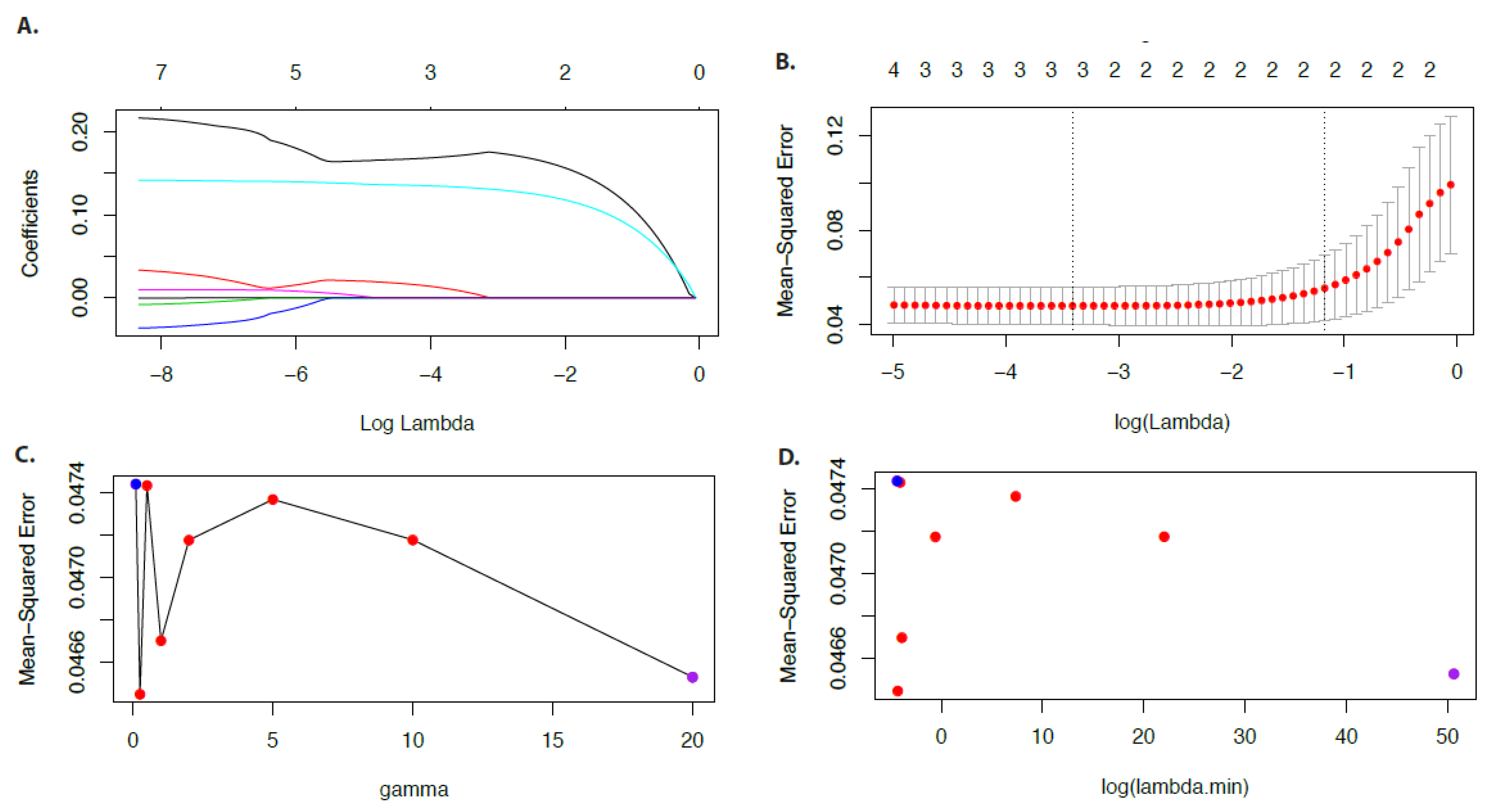
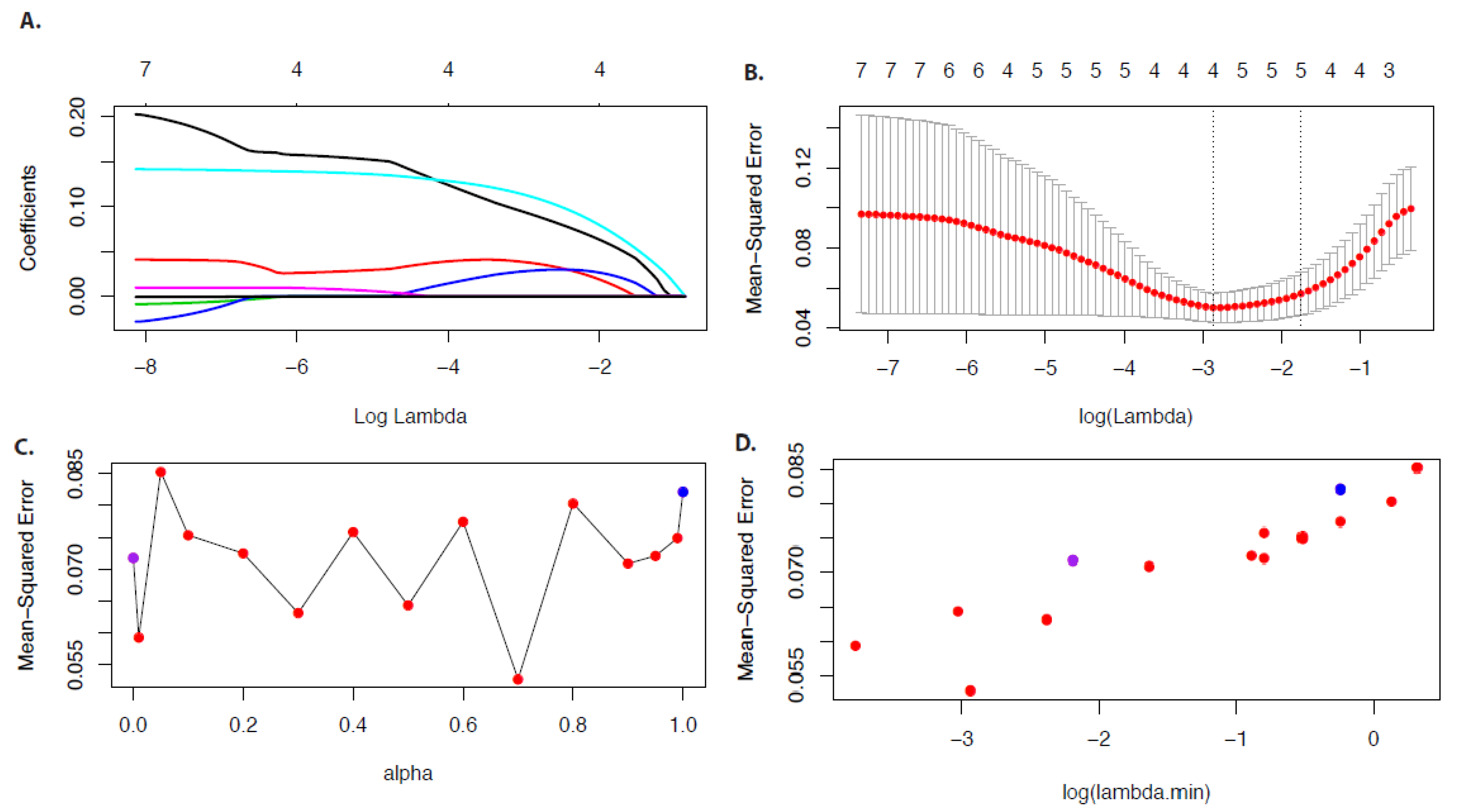
9.1. Example

In Figure 6 we show results for the economy data for $\gamma =1$. In Figure 6A we show the coefficient paths in dependence on $log\left(\lambda \right)$ and in Figure 6B the results for the mean-squared error. One can see the shrinking and selecting property of the adaptive LASSO because the regression coefficients become smaller for decreasing values of $\lambda$ and some even vanish.

For the above results we used $\gamma =1$, however, $\gamma$ is a tuning parameter that can be estimated from the data. Specifically, in Figure 6C,D we repeated our analysis for different values of $\gamma$. From Figure 6C one can see that the minimal mean-squared error is obtained for $\gamma =0.25$ but $\gamma =1.0$ also gives good results. In Figure 6D we show the same results as in Figure 6C but for the mean-squared error in dependence on ${\lambda }_{min}$. There, one sees that the ${\lambda }_{min}$ for large values of $\gamma$ are quite large.

9.2. Applications in the Literature

The adaptive LASSO has also been applied to many different problems. For instance, in genomics the adaptive LASSO has been above all used to analyze quantitative trait loci (QTL) based on SNP (Single Nucleotide Polymorphism) measurements [7,53,54,55]. It has also been applied to analyze clinical data [10,56,57] of various diseases, including cardiovascular and liver disease, and to assess organ transplantation [58].

9.3. R Package

A practical analysis for the adaptive LASSO can be performed using the glmnet R package [28].

10. Elastic Net

The elastic net regression model has been introduced by [17] to extend the LASSO by improving some of its limitations, especially with respect to the variable selection. Importantly, the elastic net encourages a grouping effect, keeping strongly correlated predictors together in the model. In contrast, the LASSO tends to split such groups keeping only the strongest variable. Furthermore, the elastic net is particularly useful in cases when the number of predictors (p) in a data set is much larger than the number of observations (n). In such a case, the LASSO is not capable of selecting more than n predictors but the elastic net has this capability.

Assuming standardized regressors and response, the elastic net solves the following problem:

$$\begin{array}{}\mathrm{(36)}& \hfill \widehat{\mathit{\beta }}& =& argmin\left\{\frac{1}{2N}\sum _{i=1}^N{(y_i-\sum _j{\beta }_j{x}_{ij})}^2+\lambda P_{\alpha }\left(\beta \right)\right\}\hfill \mathrm{(37)}& & =& argmin\{\frac{1}{2n}\parallel {\mathit{y}-\mathit{X}\mathit{\beta }\parallel }_2^2+\lambda P_{\alpha }\left(\beta \right)\}\hfill \mathrm{(38)}& \hfill P_{\alpha }\left(\beta \right)& =& {\alpha \parallel \beta \parallel }_2^2+(1-\alpha ){\parallel \beta \parallel }_1\hfill \mathrm{(39)}& & =& \sum _{j=1}^p\alpha {\beta }_j^2+(1-\alpha )\left|{\beta }_j\right|\hfill \end{array}$$

Here $P_{\alpha }\left(\beta \right)$ is the elastic net penalty (Zou and Hastie 2005). $P_{\alpha }\left(\beta \right)$ is a combination between the ridge regression penalty, for $\alpha =1$, and the LASSO penalty, for $\alpha =0$. This form of penalty turned out to be particularly useful in the case $p>n$, or in situations where we have many (highly) correlated predictor variables.

In the correlated case, it is known that ridge regression shrinks the regression coefficients of the correlated predictors towards each other. In the extreme case of k identical predictors, each of them obtains the same estimates of the coefficients [48]. From theoretical considerations it is further known that the ridge regression is optimal if there are many predictors, and all have non-zero coefficients. LASSO, on the other hand, is somewhat indifferent to very correlated predictors, and will tend to pick one and ignore the rest.

Interestingly, it is known that the elastic net with $\alpha =ϵ$, for some very small $ϵ>0$, performs very similarly to the LASSO, but removes any degeneracies caused by the presence of correlations among the predictors [48]. More generally, the penalty family given by $P_{\alpha }\left(\beta \right)$ creates a non-trivial mixture between ridge regression and the LASSO. When for a given $\lambda$, one decreases $\alpha$ from 1 to 0, the number of regression coefficients equal to zero increases monotonically from 0 (full (ridge regression) model) to the sparsity of the LASSO solution. Here sparsity refers to the fraction of regression coefficients equal to zero. For more detail, see Friedman et al. [48] providing also an efficient implementation of the elastic net penalty for a variety of loss functions.

10.1. Example

In Figure 7 we show results for the economy data for $\alpha =0.7$. Figure 7A shows the coefficient paths in dependence on $log\left(\lambda \right)$ and Figure 7B the mean-squared error in dependence on $log\left(\lambda \right)$.

Due to the fact that $\alpha$ is a parameter one needs to choose an optimal value. For this reason, we repeat the analysis for different values of $\alpha$. Figure 7C,D show the results for the mean-squared error in dependence on $\alpha$ and the mean-squared error in dependence on $log\left({\lambda }_{min}\right)$. In these figures, $\alpha =1.0$ corresponds to a ridge regression (blue point) and $\alpha =0$ corresponds to the LASSO (purple point). As one can see, an $\alpha$ value of $0.7$ leads to the minimal value of the mean-squared error and, hence, the optimal value of $\alpha$.

10.2. Discussion

The elastic net has been introduced to counteract the drawbacks of the LASSO and ridge regression. The ideas was to use a penalty for the elastic net which is based on a combined penalty of the LASSO and ridge regression. The penalty parameter $\alpha$ determines how much weight should be given to either the LASSO or ridge regression. An elastic net with $\alpha =1.0$ performs a ridge regression and an elastic net with $\alpha =0$ performs the LASSO. Specifically, several studies [59,60] showed that:

• In the case of correlated predictors, the elastic net can result in lower mean squared errors compared to ridge regression and the LASSO.
• In the case of correlated predictors, the elastic net selects all predictors whereas the LASSO selects one variable from a correlated group of variables but tends to ignore the remaining correlated variables.
• In the case of uncorrelated predictors, the additional ridge penalty brings little improvement.
• The elastic net identifies correctly a larger number of variables compared to the LASSO (model selection).
• The elastic net has often a lower false positive rate compared to ridge regression.
• In the case $p>n$, the elastic net can select more than n predictor variables whereas the LASSO selects at most n.

The last point means that the elastic net is capable of performing group selection of variables, at least to a certain degree. For further improving this property the group LASSO has been introduced (see below).

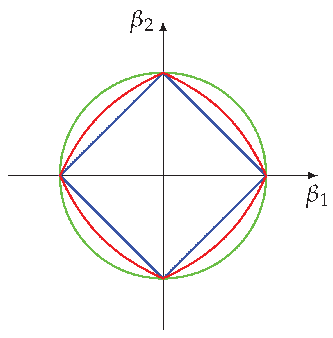
It can be shown that the elastic net penalty is a convex combination of the LASSO penalty and the ridge penalty. Specifically, for all $\alpha \in (0,1)$ the penalty function is strictly convex. In Figure 8, we visualize the effect of the tuning parameter $\alpha$ on the regularization. As one can see, the elastic net penalty (in red) is located between the LASSO penalty (in blue) and the ridge penalty (in green).

The orthonormal solutions of the elastic net is similar to the LASSO in Equation (26). It is given by [17]

$$\begin{array}{c}\hfill {\widehat{\beta }}_i^{EN}(\lambda ;orth)=\mathrm{sign}\left(\widehat{{\beta }_i^{OLS}}\right)\frac{S(\widehat{{\beta }_i^{OLS}},{\lambda }_1)}{1+{\lambda }_2}\end{array}$$

(40)

with $S(\widehat{{\beta }_i^{OLS}},{\lambda }_1)$ defined as:

$$\begin{array}{c}\hfill S(\widehat{{\beta }_i^{OLS}},{\lambda }_1)=\left\{\begin{array}{cc}\widehat{{\beta }_i^{OLS}}-{\lambda }_1\phantom{\infty }\hfill & \mathrm{if}\widehat{{\beta }_i^{OLS}}>{\lambda }_1\hfill \\ 0\phantom{0}\hfill & \mathrm{if}|\widehat{{\beta }_i^{OLS}}|\le {\lambda }_1\hfill \\ \widehat{{\beta }_i^{OLS}}+{\lambda }_1\phantom{\infty }\hfill & \mathrm{if}\widehat{{\beta }_i^{OLS}}<-{\lambda }_1\hfill \end{array}\right.\end{array}$$

(41)

Here the parameters ${\lambda }_1$ and ${\lambda }_2$ are connected to $\lambda$ and $\alpha$ in Equation (36) by

$$\begin{array}{c}\hfill \alpha =\frac{{\lambda }_2}{{\lambda }_1+{\lambda }_2}\end{array}$$

(42)

$$\begin{array}{c}\hfill \lambda ={\lambda }_1+{\lambda }_2\end{array}$$

(43)

resulting in the alternative form of the elastic net

$$\begin{array}{c}\hfill \widehat{\mathit{\beta }}=argmin\{\frac{1}{2n}\parallel {\mathit{y}-\mathit{X}\mathit{\beta }\parallel }_2^2+{\lambda }_2{\parallel \beta \parallel }_2^2+{\lambda }_1{\parallel \beta \parallel }_1\}.\end{array}$$

(44)

In contract to the LASSO in Equation (26), only the slope of the line for $|\widehat{{\beta }_i^{OLS}}|>{\lambda }_1$ is different due to the denominator $1+{\lambda }_2$. That means the ridge penalty, controlled by ${\lambda }_2$, performs a second shrinkage effect on the coefficients. Hence, an elastic net performs a double shrinkage on the coefficients, one from the LASSO penalty and one from the ridge penalty. Hence, from Equation (40) one can also see the variable selection property of the elastic net, similar to the LASSO.

10.3. Applications in the Literature

Due to the improved characteristics of the elastic net over the LASSO, this method is frequently preferred. For instance, in genomics it has been used for genome-wide association studies (GWAS) studying SNPs [7,61,62,63]. Gene expression data have also been studied, e.g., to identify prognostic biomarkers for breast cancer [64] or for drug repurposing [65]. Furthermore, electronic patient health records have been analyzed for predicting patient mortality [66]. In imaging, resting state functional magnetic resonance imaging (RSfMRI) was studied to identify patients with Alzheimer’s disease [67]. In finance, elastic nets have been used to define portfolios of stocks [68] or to predict the credit ratings of corporations [69].

10.4. R Package

A practical analysis of the elastic net can be performed using the glmnet R package [28].

11. Group LASSO

The last modern regression model we are discussing is the group LASSO, introduced by [18]. The group LASSO is different to the other regression models because it focuses on groups of variables instead of individual variables. The reason for this is that there are many real-world application problems related to, e.g., pathways of genes, portfolios of stocks, or substage disorders of patients, which have substructures, whereas a set of predictors forms a group that either should have nonzero or zero coefficients simultaneously.

The various forms of group lasso penalty are designed for such situations.

Let us suppose that the p predictors are divided into G groups, and $p_g$ is the number of predictors in group $g\in \{1,\dots ,G\}$. The matrix ${\mathit{X}}_g\in {\mathbb{R}}^{n\times p_g}$ represents the predictors corresponding to group g and the corresponding regression coefficient vector is given by ${\mathit{\beta }}_g\in {\mathbb{R}}^{p_g}$.

The group LASSO solves the following convex optimization problem:

$$\begin{array}{ccc}\hfill \widehat{\mathit{\beta }}& =& argmin\{\frac{1}{2n}\parallel \mathit{y}-\sum _{g=1}^G{\mathit{X}}_g{\beta }_g{\parallel }_2^2+\lambda \sum _{g=1}^G\sqrt{p_g}{\parallel {\mathit{\beta }}_g\parallel }_2\}\hfill \end{array}$$

(45)

Here the term $p_g$ accounts for the varying group sizes. If $p_g=1$ for all groups g, then the group LASSO becomes the ordinary LASSO. If $p_g>1$, the group LASSO works like the LASSO but on the group level, instead of the individual predictors.

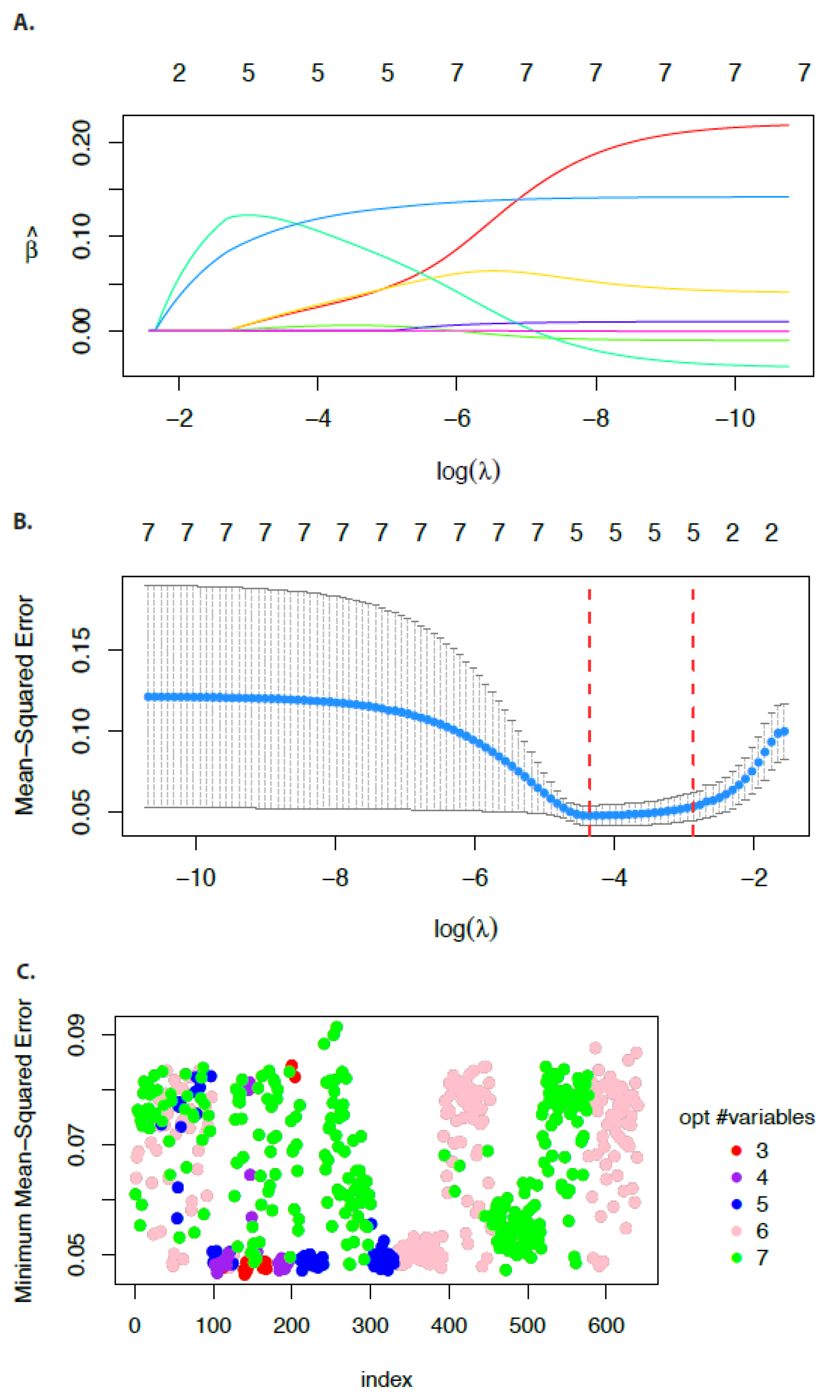
11.1. Example

In Figure 9 we show results for the economy data for the group labels $\{1,1,1,2,2,3,3\}$ for the seven predictors. Figure 9A shows the coefficient paths in dependence on $log\left(\lambda \right)$ and Figure 9B the mean-squared error in dependence on $log\left(\lambda \right)$. From the number of variables above each figure, one can see that 1 and 3 never appear. The former is for principle reasons not possible because the smallest group (labeled by ’2’ or ’3’) consists of two predictors and the latter does just not occur in this example because the group labeled by ’1’ (consisting of three predictors) is added later to the model for larger $\lambda$ values. Hence, there are jumps in the number of predictors.

Due to the fact that for this data set no obvious grouping of the predictors is available, we repeat the above analysis for 640 different group definitions for two to three different groups. In Figure 9C we show the results for this analysis. The y-axis shows the minimum mean-squared errors of the corresponding models corresponding to ${\lambda }_{min}$. The x-axis enumerates these models from 1 to 640 and the legend gives the color code for the optimal number of variables that minimize the MSE.

The last analysis demonstrates also a problem of the group LASSO because if the group definitions of the predictors are not known or cannot be obtained in a natural way, e.g., by interpretation of the problem under investigation, searching for the optimal grouping of the predictors becomes, even for a relatively small number of variables, computationally demanding due to the large number of possible combinations.

11.2. Discussion

• The group LASSO has either zero coefficients of all members of a group or non-zero coefficients.
• The group LASSO cannot achieve sparsity within a group.
• The groups need to be predefined, i.e., the regression model does not provide a direct mechanism to obtain the grouping.
• The groups are mutually exclusive (non-overlapping).

Finally, we just want to briefly mention that to overcome the limitation of the group LASSO to obtain sparsity within a group (point (2)), the sparse group LASSO has been introduced by [70]. The model is defined by:

$$\begin{array}{ccc}\hfill \widehat{\mathit{\beta }}& =& argmin\{\frac{1}{2n}\parallel \mathit{y}-\sum _{g=1}^G{\mathit{X}}_g{\mathit{\beta }}_g{\parallel }_2^2+(1-\alpha )\lambda \sum _{g=1}^G\sqrt{p_g}\parallel {\mathit{\beta }}_g{\parallel }_2+\alpha \lambda {\parallel \mathit{\beta }\parallel }_1\}\hfill \end{array}$$

(46)

For $\alpha \in [0,1]$ this is a convex optimization problem combining the group LASSO penalty (for $\alpha =0$) with the LASSO penalty (for $\alpha =1$). Here $\mathit{\beta }\in {\mathbb{R}}^p$ is the complete coefficient vector.

11.3. Applications in the Literature

Examples for applications of the group LASSO can be found above all in genomics where groups can be naturally defined via biological processes to which genes are belonging. For instance, the group LASSO has been applied to GWAS data [71,72] and gene expression data [70,73].

11.4. R Package

A practical analysis of the group LASSO can be performed using the oem R package [74,75]. Also, the gglasso R package performs a group LASSO [76].

12. Summary

In this paper, we surveyed modern regression models that extend OLS regression. In contrast to the OLS regression and ridge regression, all of these models are computational in nature because the solution to the various regularizations can only be found by means of numerical approaches.

In

Table 1. Summary of key features of the regression models.

Method	Analytical Solution	Variable Selection	Can Select $>\mathit{n}$	Grouping	Oracle
ridge regression	yes	no	yes	yes	no
non-negative garotte	no	yes	no	no	no
LASSO	no	yes	no	no	no
Dantzig selector	no	yes	yes	no	no
adaptive LASSO	no	yes	no	no	yes
elestic net	no	yes	yes	yes	no
group LASSO	no	yes	yes	yes	no

, we summarize some key features of these regression models. A common feature of all extensions of OLS regression and ridge regression is that these models perform variable selection (coefficient shrinkage to zero). This allows to obtain interpretable models because the smaller the number of variables in a model, the easier it is to find plausible explanations. Considering this, the adaptive LASSO has the most satisfying properties because it possesses the oracle property, making it capable to identify only the coefficients that are non-zero in the true model.

In general, one considers data as high-dimensional if either (I) p is large or (II) $p>n$ [59,77,78]. The case (I) can be handled by all regression models, including the OLS regression. However, case (II) is more difficult because it may require to select more variables than samples are available. Only ridge regression, Dantzig selector, elastic net, and the group LASSO are capable of this, and the elastic net is particularly suited for this situation.

Finally, the grouping of variables is useful, e.g., in cases when variables are highly correlated with each other. Again ridge regression, the elastic net, and the group LASSO have this property, and the group LASSO has been specifically introduced to deal with this problem.

In

Table 2. Overview of regularization or penalty terms and methods utilizing them.

Regularization Term	Method
L2 norm: ${\parallel \mathit{\beta }\parallel }_2$	ridge regression
L1 norm: ${\parallel \mathit{\beta }\parallel }_1$	LASSO
Lq norm: ${\parallel \mathit{\beta }\parallel }_q$	bridge regression
weighted L1 norm: ${\sum }_{j=1}^p{w}_j\left|{\beta }_j\right|$	adaptive LASSO
$c_1{\parallel \mathit{\beta }\parallel }_1+c_2{\parallel \mathit{\beta }\parallel }_2^2$	elastic net
${\sum }_{g=1}^G\sqrt{p_g}{\parallel {\beta }_g\parallel }_2$	group LASSO

, we summarize the regularization terms of the different models. From this one can understand why the number of new regularized regression models exploded in recent years because these models explore different forms of the Lq-norm or combine different norms with each other. This proved a very rich source of inspiration and new models are still under development.

We did not include the non-negative garotte and the Dantzig selector in this table because these models have a different form of the RSS term.

Regarding practical applications of these regularization regression models, the following is important to note:

Specifically, the characteristics of a data set have a strong influence on the performance of a regression model. For this reason, for practical applications it is strongly advisable to perform a comparative analysis of different models for a particular data set under investigation by means of cross validation (CV), potentially in combination with simulation studies that mimic the characteristics within this data set. Furthermore, it would be beneficial to analyze more than one data set (validation data) of the same data type to obtain reliable estimates of the variabilities among the covariates. Only in this way is it possible to guard against false assumptions leading to the selection of a suboptimal model for the data set under investigation.

13. Conclusions

Regression models find widespread applications in science and our digital society. Over the years, many different regularization models have been introduced, where each addresses a particular problem, making no one method dominant over the others, since they all have specific strengths and weaknesses. The LASSO and related models are very popular tools in this context that form core methods of modern data science [79]. Despite this, there is a remarkable lack in the literature regarding accessible reviews on the intermediate level. Our review aims to fill this gap, with a particular focus on the regularization terms.