Real-Time Vehicle Make and Model Recognition System


Faculty of Engineering and Applied Science, University of Regina, Regina, SK S4S 0A2, Canada
*
Author to whom correspondence should be addressed.
Mach. Learn. Knowl. Extr. 2019, 1(2), 611-629; https://0-doi-org.brum.beds.ac.uk/10.3390/make1020036
Submission received: 29 January 2019
/
Revised: 13 April 2019
/
Accepted: 15 April 2019
/
Published: 17 April 2019
(This article belongs to the Section Data)
Abstract
:A Vehicle Make and Model Recognition (VMMR) system can provide great value in terms of vehicle monitoring and identification based on vehicle appearance in addition to the vehicles’ attached license plate typical recognition. A real-time VMMR system is an important component of many applications such as automatic vehicle surveillance, traffic management, driver assistance systems, traffic behavior analysis, and traffic monitoring, etc. A VMMR system has a unique set of challenges and issues. Few of the challenges are image acquisition, variations in illuminations and weather, occlusions, shadows, reflections, large variety of vehicles, inter-class and intra-class similarities, addition/deletion of vehicles’ models over time, etc. In this work, we present a unique and robust real-time VMMR system which can handle the challenges described above and recognize vehicles with high accuracy. We extract image features from vehicle images and create feature vectors to represent the dataset. We use two classification algorithms, Random Forest (RF) and Support Vector Machine (SVM), in our work. We use a realistic dataset to test and evaluate the proposed VMMR system. The vehicles’ images in the dataset reflect real-world situations. The proposed VMMR system recognizes vehicles on the basis of make, model, and generation (manufacturing years) while the existing VMMR systems can only identify the make and model. Comparison with existing VMMR research demonstrates superior performance of the proposed system in terms of recognition accuracy and processing speed.
1. Introduction
Transportation of goods and people is vital activities in the contemporary world. Transportation contributes to economic prosperity and quality of life. It also has its adverse effects like pollution, resource consumption, fatigue due to driving and traffic congestions, and personal safety risks due to accidents. The projection of the global vehicle count is an inexact process, but studies have shown an exponential increase. The estimated current global vehicle count is over 1.2 billion and, according to studies, this number will cross 2 billion in 2035 [1] or in 2040 [2]. Due to the increasing number of vehicles, automated vehicle analysis is an important task in many applications.
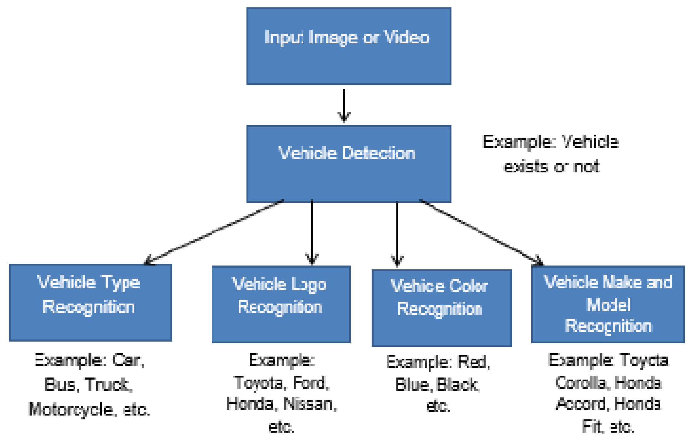
The taxonomy of vehicle analysis is depicted in Figure 1. Vehicle analysis starts with the vehicle detection. Once the vehicle is detected, we can classify it based on its class (car, bus, truck, etc.), make (Toyota, Honda, Ford, etc.), color (white, black, red, grey, etc.), or make and model (Toyota Corolla, Hando Accord, Ford Fusion, etc.). Autonomous vehicles and driver assistance, surveillance, traffic management, and law enforcement are a few of the applications taking benefit from automatic vehicle analysis. It is inconceivable for humans to monitor, observe, and analyze the ever-increasing number of vehicles manually, especially in urban environments. In contrast to the human operator, the computer vision application can monitor traffic for a longer period of time without any fatigue. The associated cost of computer applications is less and can be scaled to achieve the desired performance/cost ratio.
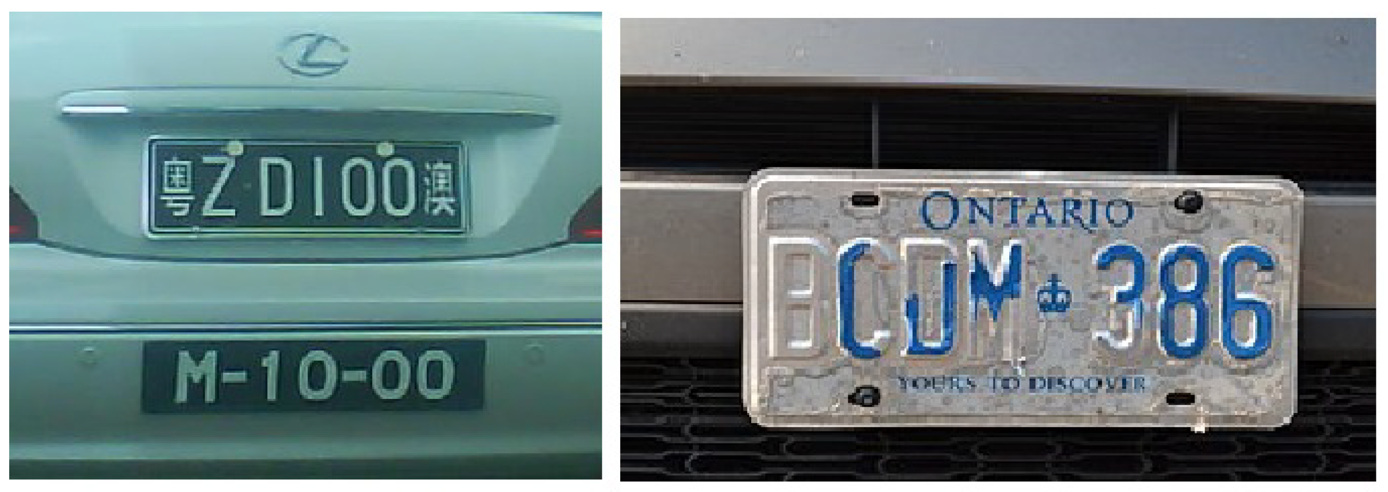
Automatic License Plate Recognition (LPR) systems present common computer vision applications that are widely deployed across the world. LPR is a well-understood problem with compelling recognition accuracy rates. LPR systems are installed in many countries for different purposes like law enforcement, electronic toll collection, crime deterrent, traffic control, etc. LPR systems identify a vehicle based on attached license plate. However, when two license plates are swapped, the LPR system will still recognize both license plates but is, inherently, incapable of recognizing the true identity. License plates can be easily forged, occluded, and damaged. Three examples where it is nearly impossible to recognize the identity of the vehicle are given in Figure 2. In the absence of an augmenting system that links license plate numbers to a vehicle make and model, the current LPR systems remain vulnerable to many malicious attacks. In many police activities like responding to a hit and run accident, an amber alert, or a hot pursuit; the vehicle make and model are typically available regardless of the lighting conditions. The license plate number might also be recognized by an eyewitness, but sometimes it is not observed or only partially observed.
A Vehicle Make and Model Recognition (VMMR) system provides great value in terms of vehicle monitoring and identification based on the appearance of the vehicle instead of the attached license plate. Authorities can query the VMMR system based on the vehicle’s description or partial number plate to find all similar vehicles in a specified area during a particular time. Hence, LPR and VMMR systems can be used to complement each other.
The VMMR problem can be treated as a multi-class image classification problem, where each class represents a specific make and model. However, more challenging and diverse challenges are associated with VMMR as compared to other problems. Few of the challenges are listed below [5]:
- Image acquisition in an outdoor environment.
- Varying and uncontrolled illumination conditions.
- Varying and uncontrolled weather conditions.
- Occlusion, shadows, and reflections in captured images.
- A wide variety of available vehicle appearances.
- Visual similarities between different models of different manufacturers.
- Visual similarities between different models of the same manufacturer.
- Tiny differences depending on the generation (group of consecutive manufacturing years).
The vehicle images used in our work reflect real world situations as they are captured in diverse weather conditions, with different lighting exposures, having partial occlusion (e.g., pedestrians), and from different viewing angles. The underlying goal is to discover the ability of supervised learning to resolve the applied computer vision problem of identifying the make, model, and manufacturing year of vehicles given the stringent limitation of the problem environment. The proposed VMMR system classifies vehicles images based on make, model, and manufacturing year while the existing VMMR systems can only identify the make and model. Vehicle models typically keep the same design shape for about five years before it is modified. We are using the term generation to describe the vehicle model having the same physical appearance but manufactured over one or more years. This article is organized as follows: Section 2 discusses the related work. The detailed system design along with feature extraction, machine learning techniques and VMMR datasets are discussed in Section 3. The efficiency and performance of the proposed VMMR is discussed in Section 4. Section 5 concludes the paper and provides direction for future work.
2. Literature Review
2.1. Vehicle Detection
Vehicle detection is the basis for vehicle classification problems. Vehicle detection confirms the presence of a vehicle in an image and extracts the region of interest to eliminate the background scene. In some cases, it is not effective to use the complete vehicle as input to the classifier and only the desired region (taillights, front lights, bumper, license plate, etc.) is extracted and used. The elimination of background and unwanted vehicle’s portion enhance the vehicle classification performance. Huang et al. use background subtraction to extract the moving objects and apply image processing to discard unwanted image regions [6]. Huang et al. train the system using a deep belief network to detect the vehicles. Lu et al. use YCbCr color space for modeling the background frame and Choquet Integral to fuse the texture features with color features [7]. An adaptive selective background maintenance model is used to solve the complex conditions and variations. Faro et al. use luminosity sensors to detect the sudden variations in illuminations without affecting the time performance; background subtraction technique is used to differentiate the vehicles from the background and segmentation scheme is applied to eliminate the occlusion [8]. Chen et al. compute Speed-Up Robust Features (SURF) for original and mirrored image and compute similarities between SURF features to find the horizontal symmetry [9]. A center line is determined; every set of symmetrical SURF points and centerline represents a possible vehicle candidate. The shadow region is used to filter out weak candidates. A comprehensive survey of wide range of vehicle detection techniques can be found in [10].
2.2. Vehicle Type Recognition
Vehicle Type Recognition (VTR) classifies the vehicles into broad categories like car, bus, van, truck, bike, etc.; the exact make and model of the vehicle is not identified in VTR. An automated VTR system is helpful in applications like urban traffic studies and analysis, electronic toll collection, etc. Wang et al. use the geometrical information to construct features and adopt simple Euclidean distance-based matching to categorize the vehicle into three types [11]. Dong et al. propose a two-level semi-supervised Convolution Neural Network (CNN) to learn local and global features and utilize softmax regression to categorize the vehicles in six classes [12]. Fu et al. propose a VTR system based on hierarchical multi-SVMs and can handle complex traffic scenes and partial occlusion [13]. Irhebhude et al. combine a local binary pattern histogram, Histogram of Oriented Gradient (HOG) and region features and use correlation-based feature selection to select discriminative features [14]. They use a support vector machine (SVM) to classify the vehicles into four categories.
2.3. Vehicle Make and Model Recognition
Classical VMMR research classifies vehicles based on make and model only. Classical systems use local features to represent the vehicle’s region of interest and require these features to be converted into global features’ representation in some cases. Scale Invariant Feature Transform (SIFT) [15], SURF [16] and HOG [17] feature extraction techniques are used by many researchers. Nearest Neighbors Classifier (NNC), Artificial Neural Networks (ANN), and Support Vector Machine (SVM) are the most widely used classifiers for VMMR systems.
Boukerch et al. presented a real-time VMMR system and evaluated it in [18]. SVM is used as single multiclass classifier and ensemble of the multi-class classifier. In this approach, the authors describe SURF features dictionary for global representation. They evaluate two dictionary building approaches; single dictionary and modular dictionary and report an accuracy rate of 94.5% with a processing speed of 7.4 images per second. Noppakun Boonsim and Simant Prakoonwit propose a one-class classifier-based approach under limited lighting [19]. The proposed approach uses one-class SVM, decision tree, and K-Mean Nearest Neighbor (KNN) for classification and a majority vote of three is used for final prediction. They use rear view images to evaluate their proposed system. A grid-based method is used for shape features and aspect ratios of different attributes of taillight and license plate are used to represent geographical features. A genetic algorithm is used for feature subset selection which improves the accuracy slightly from 93.4% to 93.8%.
Edges based features are explored in [20,21,22,23,24]. In these approaches, dependence on edges can lead to failure of the system due to occlusion. Petrovic et al. concatenate the raw pixels, Sobel edges, edge orientation, Harris corner response, normalized gradient and other image features to build feature vector and apply principal component analysis to reduce the dimensionality of the feature vector [20]. The Nearest Neighbors method is used to classify the vehicle make and models. Pearce et al. use KNN and Naïve Bayes for classification and use canny edges, Harris corners and Square Mapped Gradient (SMG) to construct the feature vector [21]. They propose to concatenate Locally Normalized Harris Strengths (LNHS) or SMG for global representation. The authors use the small and simplistic dataset to evaluate the proposed system. Vajas et al. [22] also use concatenated SMG for global representation and Clady et al. [23] use concatenated oriented contour points from Sobel edges. Both Vajas and Clady use Nearest Neighbors as a classifier for their proposed VMMR system. Munroe et al. use canny edges and classify using several techniques like KNN, ANN, C4.5, and decision trees [24].
SIFT based VMMR systems are proposed in [25,26,27,28]. Psyllos et al. use a two-step approach [28]. They use phase congruency to identify the vehicle logo and then SIFT features to identify the specific model. Probabilistic Neural Networks are used for classification. The authors test the proposed approach against simple and non-occluded images. Different viewpoints and variation in illumination are also not considered. Even then a low accuracy rate of 54% is reported. Dlagnek use SIFT and a brute force matching algorithm in his work [25]. Exhaustive matching, used in this work, is a very time-consuming process. Baran et al. use SIFT, SURF and HOG features and define dictionaries for global feature representation [26]. Baran use multi-class SVM with very large dictionaries to represent the input images. Fraz et al. extract SIFT features and form a lexicon comprising of all the features from training dataset as words [27]. Fisher encoded representation is used to compute the lexicon for image features, SIFT. The Fisher encoded scheme is computationally expensive and the authors report the processing time of about 0.4 s for every image. Jang et al. use SURF features and bag-of-words model for global feature representation [29]. The authors have created a dataset using multiple toy cars and a structured matching technique for classification.
A global feature representation based on a grid pattern is proposed in [9,30]. Hsieh et al. divide input image into a grid and compute SURF and HOG for each block independently [30]. The authors train ensemble of SVM and combine the results to determine the final decision. Chen et al. [9] compute HOG features for the grid-based pattern and concatenate HOG features for global representation. By testing our system with their dataset, we show that our system performs well in terms of recognition accuracy and processing speed. The grid-based schemes assume a fixed camera and are prone to failures in cases where the camera height, pitch or yaw may change, resulting in vehicle views which the system might not be trained for.
3. Materials and Methods
3.1. Dataset
Pearce and Pears [21] create a dataset having 177 images from 21 vehicle classes; each vehicle class consists of five or more images. Eighty-five more images are added from other uncommon vehicle classes (53 classes); each class having one or two images. Testing dataset is created by applying ‘leave-one-out’ scheme over 177 images. Jang and Turk [29] use 20 toy cars to create the dataset. They capture images from 16 different viewpoints for each toy car. The training dataset is created with 2650 images and the proposed VMMR is tested with 801 images. Psyllose et al. [28] create a training dataset with 10 classes, each class having five images. An unknown class with five images is also added to training dataset. Testing dataset is created with the same pattern except each class contains 10 images. Jonathan Boyle and James Ferryman [31] create a dataset for side view vehicle images. The side view vehicles dataset is comprised of more than 10,000 images with 86 make/model categories. The authors use 50% of images of each class with an upper limit of 200 images for the training purposes while the rest of the images are used for testing. Baran et al. [26] create the dataset by downloading images from the internet or capturing images outdoor. The training dataset has 17 vehicle classes and 80 images for each class; thus, 1360 images are available for the training process. The testing dataset consists of 2499 images. The testing dataset has images with degraded quality and lesser resolution as compared to the training dataset. There is no occlusion in images.
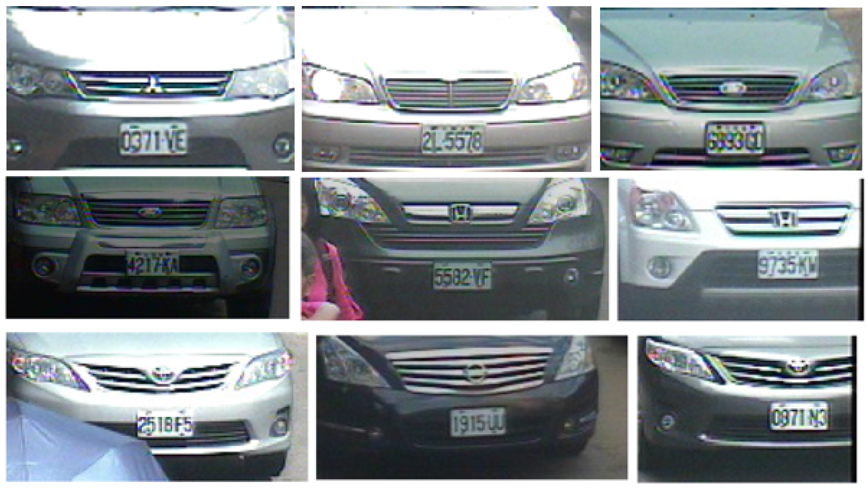
We adopt a realistic and publicly available dataset—the National Taiwan Ocean University-Make and Model Recognition (NTOU-MMR) dataset [9]. The NTOU-MMR dataset is used in multiple studies like [9,18]. Chen et al. [9] propose a VMMR system using symmetrical SURF and created a dataset under Vision Based Intelligent Environment (VBIE) project [32] in 2014 and named it the NTOU-MMR dataset. The dataset can be accessed at [33]. Jabbar et al. [18] use the NTOU-MMR dataset in their work. Hence, we can compare our VMMR performance with Chen et al. [9] and Jabbar et al. [18]. The dataset is divided into a testing and training dataset and vehicles are divided into twenty-nine different classes based on make and model. Vehicles belonging to six manufacturers are available in NTOU-MMR dataset; the manufacturers are Toyota, Ford, Mitsubishi, Honda, Suzuki, and Nissan. Few of the sample images are shown in Figure 3 to illustrate the variability of the dataset. The NTOU-MMR dataset provides the following characteristics which motivated us to use it to train and evaluate our VMMR system. We believe the five listed characteristics bring the NTOU-MMR dataset closer to real-life situations compared to other datasets available:
- The dataset contains images of stationary and moving vehicles with a speed up to 65 km/h.
- The dataset images contain vehicles with several viewing angles ranging from degrees to degrees relative to a scene directly from the front of a vehicle.
- The dataset images are captured throughout daytime and nighttime.
- The dataset is created with varying weather conditions between sunny, rainy and cloudy.
- Some of the vehicles are partially occluded by an irrelevant object like a pedestrian.
Vehicles’ classes are defined based on make and model in this dataset; we added generation to fit the dataset with our vision. We have divided the dataset into classes based on make, model and generation of vehicles. Now, the dataset is divided into thirty-five classes. The detailed description of the dataset is given in Table 1 that lists the number of images available for training and testing process. The NTOU-MMR dataset has a few problems such as the small number of training images for a few categories. There are no testing images available for Toyota RAV4 in the original dataset. We use the dataset as it is available except the change made in the number of classes.
3.2. Hardware and Software Platform
We have used an Intel®Core™i7 processor (3.4 GHz) with 16 GB of RAM to perform all our experiments. The VMMR is implemented using MATLAB®R2012a on a 64-bit Microsoft Windows 7 operating system.
3.3. Methodology
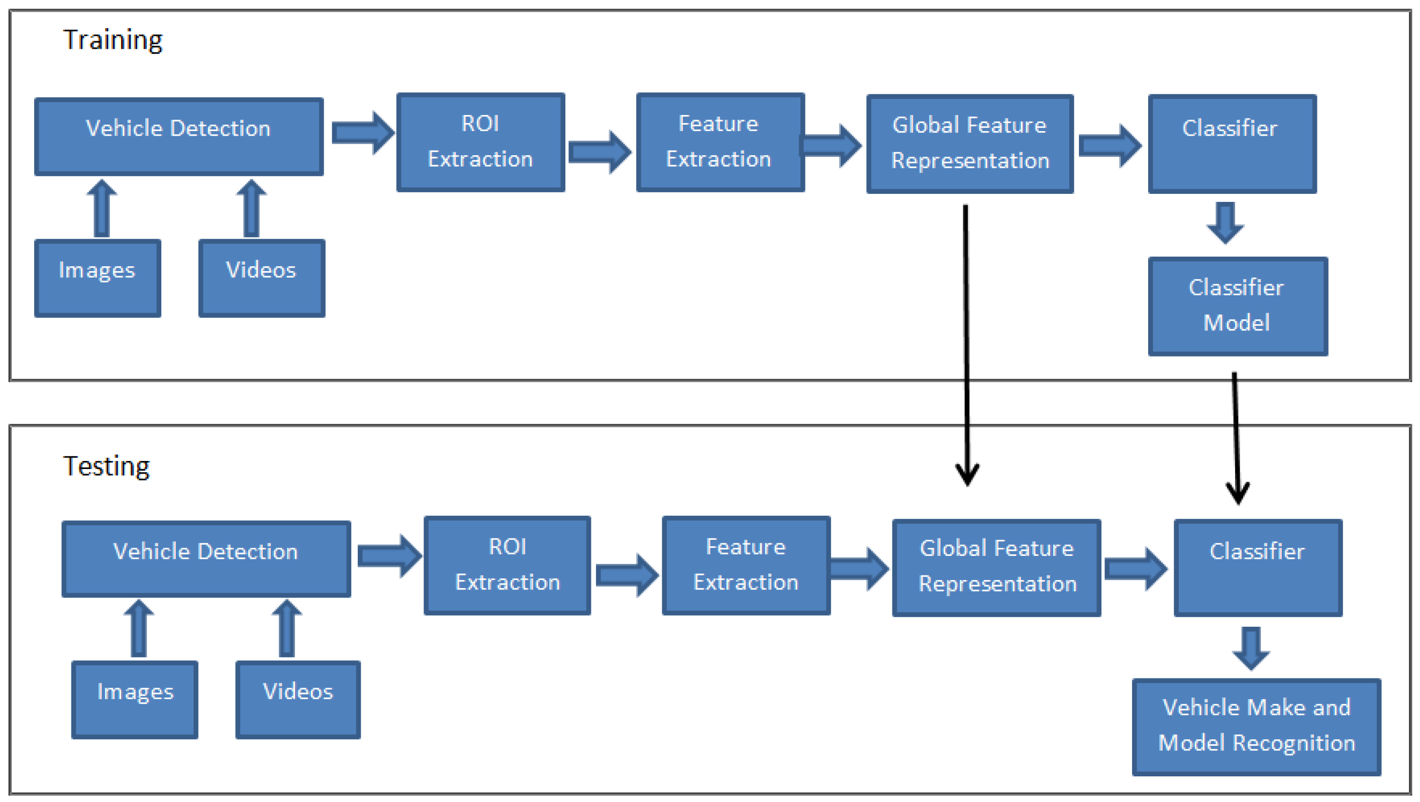
We develop a real-time VMMR system based on machine learning and computer vision techniques. Computer vision techniques are used to express images in fewer attributes that characterize vehicles. Machine learning techniques are used to classify the vehicles. The overall architecture of vehicle classification system is given in Figure 4. The VMMR system is divided into two subsystems: training subsystem and testing/classification subsystem. The training subsystem is used to train the VMMR engine using a subset of the available dataset, whereas the classification subsystem recognizes make and model of vehicles in new images never used for training. Vehicle detection, Region of Interest (ROI) Extraction and feature extraction are common for both training and testing tasks. Global feature representation and classification components are different in the training process than in the testing process. The global feature representation module may generate a model for the encoding of images’ features depending on the applied technique. Similarly, the classifier module produces a model as a result of the training process that is then used by the testing module to predict the outcome for the newly examined images. Hence, the arrows from the training process to the testing process represent the usage of models in testing process created during the training process. The proposed system works without the global feature representation component. The extracted features are directly fed into the classifier. The omission of the global feature representation component improves the processing speed of the VMMR without degrading the recognition accuracy.
The input to the system can be either images or videos. In case of videos, frames can be extracted at regular intervals. The vehicle detection module verifies the existence of a vehicle in the current image and the vehicle detection process also localizes the vehicle within the image. If a vehicle exists in the image, it is further processed; otherwise, the image is discarded. We define the ROI to represent the part of the vehicle in the image that provides the discriminative and prominent features. The discriminative and prominent features are easily distinguishable between different vehicles. We have the frontal vehicle images in our work to design the VMMR and used bumper, front lights, and bonnet area as ROI in our work as shown in Figure 3. The ROI extraction module removes the background as well as part of the vehicle from any given image that is not helpful during classification and can degrade the classification performance. We use a vehicle detection technique proposed by Chen et al. [9] for vehicle detection and ROI extraction.
The next step is to extract features from the input image. Features provide an image representation method that is more suitable for computer models such as machine learning and pattern recognition applications. The features are used to represent a scene or the uniqueness of an object. Once the prominent interest points are determined, feature descriptors are computed for the interest points. The feature descriptor provides a robust and invariant representation for the interest points. Various feature extraction and descriptors are available in the literature. We use HOG and GIST image features in this work. Feature extraction techniques may extract a variable number of features in an image. Global feature representation is the process to combine all the extracted feature points to represent an entire image feature. Global feature representation generates an image feature vector which represents all images with the same dimensionality and the same pattern. Lastly, the VMMR uses a supervised learning to enforce the image classification on the learning engine. The classifier is trained using image feature vectors generated for the training dataset and new incoming observations are then categorized using the trained classifier. The classifier’s performance can be measured in terms of correctly identified, incorrectly identified and missed observations. The testing dataset contains the new unseen observations which are used to determine classifier’s performance in terms of a successful recognition rate.
3.4. Feature Extraction and Representation
We divide image features into two categories for VMMR problems: local features and global features. A local feature is defined on the basis of a prominent point/patch of the image. An image can have a variable number of features. A global feature is either computed based on the entire image or on every part of the image. Every image in the dataset has the same number of global features. Global feature representation techniques are applied to combine local features to construct image feature vector with the same dimensionality and pattern for every image. In case of global features, all the features are simply concatenated to create an image feature vector. Local features based VMMR system are reported in our previous works [5,34]. There is no significant performance gain (recognition rate and processing speed) of using only local features. Our experimentation with global feature representation (required for local features) reveals that it decreases the processing speed. In this work, we use HOG and GIST features which utilize entire images not just the prominent local points.
3.4.1. Histogram of Oriented Gradients
The HOG feature introduced by Dalal and Triggs [17] for robust human detection has been seen widely used for object recognition. Every object or shape in an image is composed of a collection of lines (edges), thus we can describe objects within an image by using the distribution of gradient orientations (directions). HOG divides the image into small connected and overlapped regions known as cells; the gradient directions are computed for every pixel in the region and a histogram is created for the gradient directions. Every cell’s histogram is concatenated to generate the final HOG descriptor. Normalization of feature vector results in better invariance to changes in the illumination and shadowing. The histogram representation lessens the impact of noise. We use different window sizes to create a HOG feature descriptor in our work. We do not combine multiple windows to construct a bigger overlapping block. We create a HOG descriptor with the smaller size as compared to the standard HOG descriptor which results in improved the processing speed. The standard HOG creates a feature descriptor with a size of 3780 elements for a 128 × 64 image, but the size of an HOG descriptor without overlapping is 1152 elements for the same image and same configurations. All the images in the NTOU-MMR dataset do not have the same dimensions; instead of fix sized cells, we divide every image into an equal number of cells. This technique helps us create an image feature vector using simple concatenation and without applying a global feature representation technique.
3.4.2. Gist Feature Descriptor
Humans are capable of classifying an object or scene with a glance without considering the details present in an image. For example, after viewing an image of tall buildings or trees or ocean, we can instantly recognize the scene without thinking of the details or existence of other objects. The GIST of a scene [35] refers to the information contents gathered in a glance. The GIST feature descriptor is “a low dimensional representation of the scene, which does not require any form of segmentation” [36]. The GIST descriptor was initially proposed for scene classification. SIFT and SURF focus on individual prominent points and the HOG feature descriptor is computed based on individual windows (patches) and concatenated later, whereas the GIST descriptor focuses on the shape of an entire image as a single object and calculates the feature vector. The GIST descriptor ignores the presence of local objects and their relationships. Therefore, GIST provides a holistic representation of a scene. We create GIST descriptor with four scales and eight orientation creating thirty-two transformed images. Gabor transform is applied on these thirty-two images to create feature maps and the feature maps are divided into the 4 × 4 grid or 16 blocks, which generates a 512-dimensional feature vector (16 averaged values × 32 feature maps).
3.5. Classification
Designing VMMR requires the identification of the specific vehicle in terms of its manufacturer, model, and generation. After feature extraction and image feature vector construction, the next step is to train the classifier which is used to recognize the new incoming observations. During the training phase, classifiers learn the intra-class similarities (multiple vehicles belonging to the same category) and inter-class differences (vehicles belonging to different categories) and build up a model that is used later for recognizing the unseen vehicles. Among the multiple available classifiers, none was found to perform optimally at all different types of applications [37]. Data scaling, the presence of outliers and noise, redundant attributes, overfitting, and underfitting are a few of the factors that affect most classifiers’ performance. We use SVM and Random Forest (RF) classification techniques in this work and comment on the effect of image imperfections.
3.5.1. Support Vector Machine
The SVM [38,39] is a supervised learning method and efficient binary classifier. The SVM uses a subset of training data observations, known as Support Vectors (SVs), to represent the optimal separation between two classes. SVM is robust to overfitting especially for a dataset with higher dimensions (features). SVM can perform efficiently in case of nonlinear separable data by using nonlinear kernel functions. Cover’s theorem [40] states that a nonlinear kernel function is more likely to generate a linearly separable data points in higher dimensional space when it is applied on a linearly inseparable data. More details on the characteristics of kernel functions and their construction can be found in [41]. SVM is a memory intensive algorithm and the selection of kernel can be trickier.
An ensemble of binary classifiers is used to create multi-class SVM classifier. One-versus-rest [42] and one-versus-one [43] are two approaches used for multi-class SVM classification. The results of the binary SVMs can be combined in different ways for classification, such as majority voting, least square error weighted outputs, and double layer hierarchical combination. We used one-versus-one approach in our work. Hsu and Lin have compared both approaches in [44] and concluded that both approaches have comparable performance except one-versus-one require lesser training time as compared to one-versus-rest approach.
3.5.2. Random Forest
The RF classification is ensemble learning approach proposed by Leo Breiman [45]. Weak binary decision trees are used to create an ensemble in RF Classification. RF constructs a multitude of decision trees during the training process and the final class is determined using a mode (majority voting) during the testing process. Ho [46] initially introduced the idea of the RF by using Random Subspace method [47]. Brieman combined the creation of random subsets of training data named as bagging with Ho’s idea of randomly subsampling of training features to build the decision trees. The observations in the datasets often have missing values; the features may have unavailable, corrupt or invalid values. RF classifiers produce good results on missing data [48]. RF classification does not require tree pruning and can overcome the decision trees’ problem of overfitting [48]. The increase in the number of decision trees’ results in a reduction in an overfitting problem, but, on the other hand, also results in an increase in training and testing time. RF classification is easily scalable and can model nonlinear decision boundary naturally due to their hierarchical structure.
4. Results and Discussion
VMMR uses two machine learning approaches: SVM and RF. Both image features, HOG and GIST, are used with each classifier making it four combinations. The experiments are performed multiple times and the averaged results are presented here. We discuss the computational time required for feature extraction. Then, we discuss VMMR results for each machine learning approach and feature extraction combination in terms of recognition rate and processing speed. Lastly, we compare our results with other VMMR research. The recognition rates are only computed for VMMR. The performance of vehicle detection and ROI extraction is not accumulated in the recognition rates.
The computational time is an important factor for any real-time application. The measured computational times for GIST and HOG (with different configuration) are provided in Table 2. The total time required for computing each configuration is provided in seconds per 100 images. As we increase the number of blocks in HOG the computational time increases. The training and testing datasets undergo through the same process in case of HOG and GIST features; hence, the computational time required is the same for the training and testing phases.
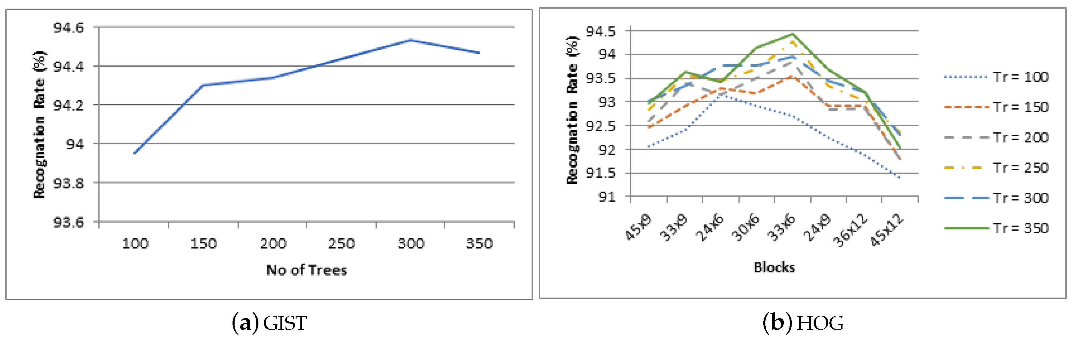
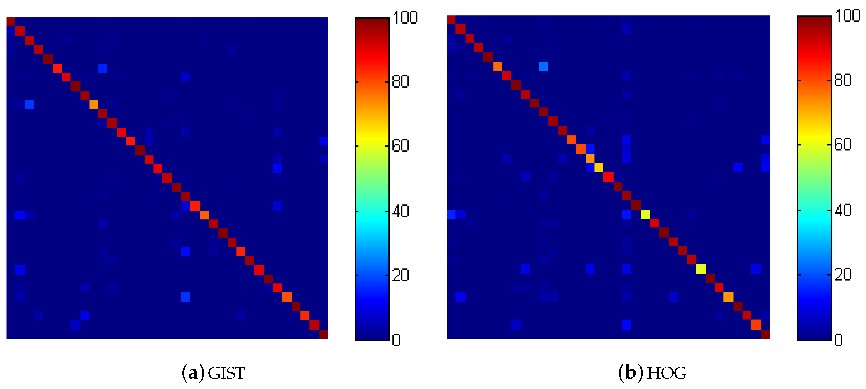
The RF is trained with configuration of 100, 150, 200, 250, 300, and 350 decision trees. We use the term RF-VMMR to refer the VMMR system with RF classification. The other two important parameters used in RF training are the number of randomly selected (with replacement) samples used to grow each decision tree and the number of randomly selected attributes to consider for each decision tree; we select the values of these two parameters based on experimental analysis. The same parameters are used during the testing phase. We observe that the recognition rate decreases if we reduce the size of training subset for RF. Hence, we use all the training dataset to grow the decision trees. Similarly, we observe that RF performs better with the number of selected attributes equal to the square root of the total number of attributes for our RF-VMMR system. The RF-VMMR recognition rates are shown in Figure 5a,b. The vertical axis of both figures represents the RF-VMMR recognition rate in percentage. The horizontal axis shows the number of decision trees used for RF training for GIST features in Figure 5a and number of blocks used to construct HOG image features in Figure 5b. The recognition rate (vehicles correctly recognized) for different RF configurations (number of decision trees) are shown using different styled lines for HOG in Figure 5b. The confusion matrices for RF-VMMR are shown in Figure 6a,b.
As depicted in Figure 5a,b, the increase in the number of decision trees in the RF algorithm increases the recognition rate initially, but, after certain thresholds, further increase in the number of decision trees negatively affects the recognition performance. Although this threshold is not fixed for all of the variations of dataset representations, in our dataset, the recognition rate decreased after 300 decision trees in most of the cases. The behavioral pattern whereby there is an increase in the recognition rate followed by decrease as the number of decision trees increases can be seen for every feature extraction technique and variation. Although there are small variations, the overall recognition rate follows the same behavioral pattern.
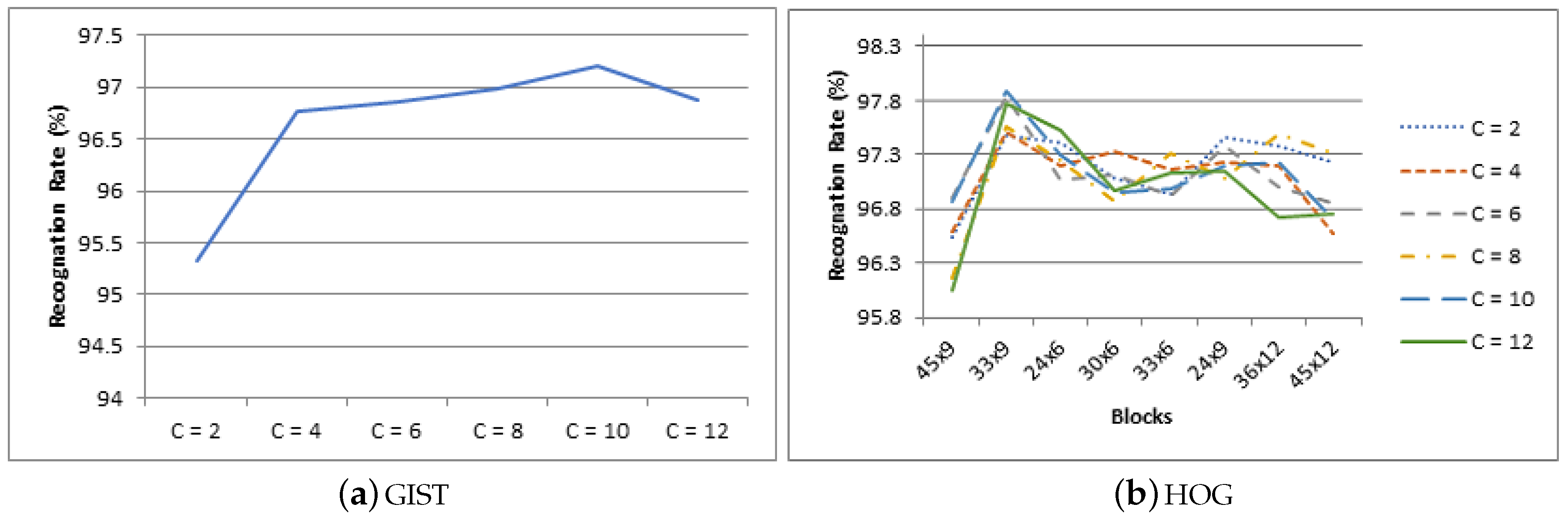
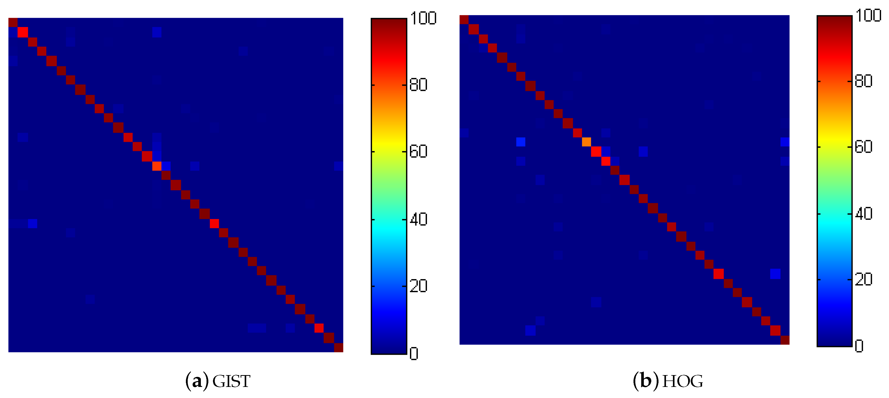
We use a linear kernel in this work. A linear kernel is a good option when the numbers of features are greater than the number of observations [49]. When applying the VMMR system to the NTOU-MMR dataset, we use 2750 training observations where the number of features varied from 512 to 5000 for each observation depending on the feature extraction technique and configuration employed. Hsu et al. reported that the mapping of data into a higher dimensional space does not improve the performance in the case of a large number of features [49]. The linear kernel also results in faster training as compared to other kernels [49]. The regularization parameter C is used to control the margin of the hyperplane separating two data classes. A larger value for C means a smaller margin between the two classes. We train the SVM algorithm with C = 2, 4, 6, 8, 10, and 12. We use the term SVM-VMMR to represent the VMMR system with SVM classification. The recognition rates for the SVM-VMMR system are shown in Figure 7a,b. The vertical axis of both figures represents the SVM-VMMR recognition rate in percentage. The horizontal axis shows the size of margin used for SVM training for GIST features in Figure 7a and number of blocks used to construct HOG image features in Figure 7b. The recognition rate for each SVM configurations (size of margin) is shown using different styled lines for HOG in Figure 7b. The confusion matrices for RF-VMMR are shown in Figure 8a,b.
As depicted in Figure 7a,b, the increase in the number of blocks increases the recognition rate up to a certain point, and, then, the recognition rate decreases. HOG achieves its best recognition rate of 94.43% with 33x6 blocks in the case of RF-VMMR (350 Decision Trees) and 97.89% with 33 × 9 blocks in the case of SVM-VMMR (C = 10). GIST achieves its best recognition rate of 94.53% in case of RF-VMMR (300 decision trees) and 97.20% in case of SVM-VMMR (C = 10). We can conclude based on the recognition rate that GIST and HOG perform similarly for RF-VMMR and SVM-VMMR in terms of recognition rate.
All the parameters are determined using the training dataset. However, we have reported all the results (performed on a testing dataset) to illustrate the effect of variation in other parameters like number of trees, C, feature extraction configuration.
The training of a VMMR system can be performed offline hence it does not put any timing constraint. The processing speed (images per second) of recognition process for RF-VMMR is provided in Table 3 and for SVM-VMMR in Table 4. The processing speeds are measured based on the accumulated values of the feature extraction and representation time and recognition phase. The first column tells about the feature extraction technique and the second column tells about its configuration. The remaining six columns provide the processing speed for different RF and SVM configurations.
The VMMR system performance depends on mainly two elements. The first element is the representation of dataset which includes the feature extraction techniques and global feature representation techniques. The second element is the machine learning classification algorithm. Both feature representation and machine learning algorithm affect the VMMR system. Observing the accuracies of SVM-VMMR and RF-VMMR, we can see that the SVM-VMMR performs better than RF-VMMR. Both features’ extraction techniques have similar performance for both classification techniques.
The real-time processing speed of the VMMR system is a key factor in performance. Every driver maintains a minimum following distance to avoid the collisions which is measured in seconds. On the highways (under normal conditions), most of the drivers normally observe the minimum following distance in between 1.5 s to 2.0 s [50]. With this minimum following distance, the number of vehicles passing through a single lane in an hour is between 1800 to 2400 or 7200 to 9600 for a four-lane highway. A real-time VMMR system installed on a four-lane highway, covering both sides, is required to process six vehicles per second approximately in order to analyze entire traffic flow. The proposed VMMR system can process 13.9 frames per second (SVM-VMMR). The processing speed reduces to 10.1 frames per second with the inclusion of computation time of vehicle detection module. The training time is not considered here as the training process is performed offline and does not impose any temporal constraint over the final system. The processing speed for GIST is almost the same in case of SVM-VMMR and RF-VMMR, whereas, for HOG features, the RF-VMMR processing speed is almost twice as fast as SVM-VMMR. The values for the number of decision trees for RF and the margin C for SVM have very little effect on the computation time for the testing phase as can be seen in Table 3 and Table 4. The difference between the processing speeds are due to the feature extraction and representation techniques. The processing speed of the RF-VMMR for the HOG features (33 × 6 blocks) is 35.7 images per second with the recognition rate of 94.43%, whereas the processing speed of the SVM-VMMR for the HOG features (33 × 9 blocks) is 13.9 images per second with the recognition rate of 97.89%. RF-VMMR and SVM-VMMR systems with GIST features yield a similar recognition rate for both systems. In addition, the processing speed is lower with GIST features than with HOG features. The feature extraction step requires more computational time which can easily be processed in parallel to increase the processing speed of the system. The time required for feature extraction is very high as compared to the RF testing process so an increase in the number of decision trees does not affect processing speed much, whereas processing speed is affected by the feature extraction configuration. The value of C can affect the training time, but, once the system is trained, all the new coming observations go through the same type of computation. Hence, the processing speed remains the same for all different values of C for the same feature extraction configuration.
The proposed VMMR systems are compared with nine other VMMR approaches in Table 5 with respect to the recognition rate and processing speed. Our VMMR systems outperform other VMMR systems, in terms of both recognition rate and processing speed. The results of our proposed VMMR systems, given in Table 5, are the best outcomes among all the feature extraction and machine learning algorithm variations. Chen et al. [9] and Jabbar et al. [18] also use the NTOU-MMR [33] dataset to test their work. Our SVM-VMMR system outperforms both of their systems in terms of recognition rate and processing speed. Most previous approaches use local features such as SIFT, SURF, edges, corners, etc. to represent the images, which may be the reason for their poorer performance.
5. Conclusions and Future Work
This work presents a real-time VMMR system with better performance than existing VMMR systems in terms of recognition rate and processing speed. A publicly available NTOU-MMR dataset based on realistic assumptions is used in this work. The dataset is modified to include a vehicle’s generation information along with make and model. We have used HOG and GIST to represent the images and SVM and RF to classify the vehicles. We have shown using the experimental analysis that our system is suitable for real-time applications with a higher recognition rate. The proposed system works well in challenging situations where vehicles are partially occluded, partially out of the image frame or poorly visible due to low lighting. This system can provide great value in terms of vehicle monitoring and identification based on vehicle appearance instead of the vehicles’ attached license plate. The existing VMMR research focuses on recognizing vehicles sufficiently to report only their make and model. We have included generation as another parameter. Thus, our VMMR system recognizes a vehicle and provides information about vehicle make, model and generation.
Although the proposed VMMR system outperforms the previous systems, it can be further enhanced. Image feature vectors have a large number of features/dimensions. Dimensionality reduction techniques can be explored to reduce this number. A publicly available better and larger dataset with more vehicle types will benefit the research in this area. Deep learning techniques can also be explored with a bigger dataset.
Author Contributions
M.A.M. conceptualized the idea, performed formal analysis and wrote the original draft. Y.M. and A.B. contributed in reviewing, editing, supervision, and resource/funding acquisition.
Conflicts of Interest
The authors declare no conflict of interest. The funders had no role in the design of the study; in the collection, analyses, or interpretation of data; in the writing of the manuscript, or in the decision to publish the results.
References
- Available online: http://www.greencarreports.com/news/1093560_1-2-billion-vehicles-on-worlds-roads-now-2-billion-by-2035-report (accessed on 5 June 2017).
- Available online: https://www.weforum.org/agenda/2016/04/the-number-of-cars-worldwide-is-set-to-double-by-2040 (accessed on 5 June 2017).
- Available online: https://commons.wikimedia.org/wiki/File:China_cross-border_Guangdong-Macau_registration_plate_%E7%B2%A4Z_D100%E6%BE%B3.jpg (accessed on 14 April 2019). (licensed under CC BY-SA 2.5).
- Available online: https://commons.wikimedia.org/wiki/File:Damaged_Ontario_DCDM236.JPG (accessed on 14 April 2019). (licensed under CC BY-SA 4.0).
- Manzoor, M.A.; Morgan, Y. Vehicle Make and Model classification system using bag of SIFT features. In Proceedings of the 2017 IEEE 7th Annual IEEE Computing and Communication Workshop and Conference (CCWC), Las Vegas, NV, USA, 9–11 January 2017. [Google Scholar]
- Huang, B.-J.; Hsieh, J.-W.; Tsai, C.-M. Vehicle Detection in Hsuehshan Tunnel Using Background Subtraction and Deep Belief Network. In Asian Conference on Intelligent Information and Database Systems; Springer: Cham, Switzerland, 2017. [Google Scholar]
- Lu, X.; Izumi, T.; Takahashi, T.; Wang, L. Moving vehicle detection based on fuzzy background subtraction. In Proceedings of the 2014 IEEE International Conference on Fuzzy Systems (FUZZ-IEEE), Beijing, China, 6–11 July 2014. [Google Scholar]
- Faro, A.; Giordano, D.; Spampinato, C. Adaptive background modeling integrated with luminosity sensors and occlusion processing for reliable vehicle detection. IEEE Trans. Intell. Transp. Syst. 2011, 12, 1398–1412. [Google Scholar] [CrossRef]
- Chen, L.-C.; Chen, J.-W.; Yan, Y.; Chen, D.-Y. Vehicle make and model recognition using sparse representation and symmetrical SURFs. Pattern Recognit. 2015, 48, 1979–1998. [Google Scholar] [CrossRef]
- Sivaraman, S.; Trivedi, M.M. Looking at vehicles on the road: A survey of vision-based vehicle detection, tracking, and behavior analysis. IEEE Trans. Intell. Transp. Syst. 2013, 14, 1773–1795. [Google Scholar] [CrossRef]
- Wang, R.; Zhang, L.; Xiao, K.; Sun, R.; Cui, L. EasiSee: Real-time vehicle classification and counting via low-cost collaborative sensing. IEEE Trans. Intell. Transp. Syst. 2014, 15, 414–424. [Google Scholar] [CrossRef]
- Dong, Z.; Wu, Y.; Pei, M.; Jia, Y. Vehicle type classification using a semisupervised convolutional neural network. IEEE Trans. Intell. Transp. Syst. 2015, 16, 2247–2256. [Google Scholar] [CrossRef]
- Fu, H.; Ma, H.; Liu, Y.; Lu, D. A vehicle classification system based on hierarchical multi-SVMs in crowded traffic scenes. Neurocomputing 2016, 211, 182–190. [Google Scholar] [CrossRef]
- Irhebhude, M.E.; Amin, N.; Edirisinghe, E.A. View invariant vehicle type recognition and counting system using multiple features. Int. J. Comput. Vis. Signal Process. 2016, 6, 20–32. [Google Scholar]
- Lowe, D.G. Object recognition from local scale-invariant features. In Proceedings of the Seventh IEEE International Conference on Computer Vision; IEEE: New York, NY, USA, 1999; Volume 2. [Google Scholar]
- Bay, H.; Ess, A.; Tuytelaars, T.; Van Gool, L. Speeded-up robust features (SURF). Comput. Vis. Image Underst. 2008, 110, 346–359. [Google Scholar] [CrossRef]
- Dalal, N.; Triggs, B. Histograms of oriented gradients for human detection. In Proceedings of the 2005 IEEE Computer Society Conference on Computer Vision and Pattern Recognition, CVPR 2005, San Diego, CA, USA, 20–25 June 2005; Volume 1. [Google Scholar]
- Siddiqui, A.J.; Mammeri, A.; Boukerche, A. Real-time vehicle make and model recognition based on a bag of SURF features. IEEE Trans. Intell. Transp. Syst. 2016, 17, 3205–3219. [Google Scholar] [CrossRef]
- Boonsim, N.; Prakoonwit, S. Car make and model recognition under limited lighting conditions at night. Pattern Anal. Appl. 2017, 20, 1195–1207. [Google Scholar] [CrossRef]
- Petrovic, V.S.; Cootes, T.F. Analysis of Features for Rigid Structure Vehicle Type Recognition. BMVC 2004, 2. [Google Scholar] [CrossRef]
- Pearce, G.; Pears, N. Automatic make and model recognition from frontal images of cars. In Proceedings of the 2011 8th IEEE International Conference on Advanced Video and Signal-Based Surveillance (AVSS), Klagenfurt, Austria, 30 August–2 September 2011. [Google Scholar]
- Varjas, V.; Tanács, A. Car recognition from frontal images in mobile environment. In Proceedings of the 2013 8th International Symposium on Image and Signal Processing and Analysis (ISPA), Trieste, Italy, 4–6 September 2013. [Google Scholar]
- Clady, X.; Negri, P.; Milgram, M.; Poulenard, R. Multi-class vehicle type recognition system. Lect. Notes Comput. Sci. 2008, 5064, 228–239. [Google Scholar]
- Munroe, D.T.; Madden, M.G. Multi-class and single-class classification approaches to vehicle model recognition from images. In Proceedings of the 16th Irish Conference on Artificial Intelligence and Cognitive Science (AICS 2005), Portstewart, Northern Ireland, September 2005. [Google Scholar]
- Dlagnekov, L.; Belongie, S.J. Recognizing Cars; Department of Computer Science and Engineering, University of California: San Diego, CA, USA, 2005. [Google Scholar]
- Baran, R.; Glowacz, A.; Matiolanski, A. The efficient real-and non-real-time make and model recognition of cars. Multimedia Tools Appl. 2015, 74, 4269–4288. [Google Scholar] [CrossRef]
- Fraz, M.; Edirisinghe, E.A.; Sarfraz, M.S. Mid-level-representation based lexicon for Vehicle Make and Model Recognition. In Proceedings of the 2014 22nd International Conference on Pattern Recognition (ICPR), Stockholm, Sweden, 24–28 August 2014. [Google Scholar]
- Psyllos, A.; Anagnostopoulos, C.-N.; Kayafas, E. Vehicle model recognition from frontal view image measurements. Comput. Stand. Interfaces 2011, 33, 142–151. [Google Scholar] [CrossRef]
- Jang, D.M.; Turk, M. Car-Rec: A real time car recognition system. In Proceedings of the 2011 IEEE Workshop on Applications of Computer Vision (WACV), Kona, Hawaii, 5–7 January 2011. [Google Scholar]
- Hsieh, J.-W.; Chen, L.-C.; Chen, D.-Y. Symmetrical SURF and its applications to vehicle detection and vehicle make and model recognition. IEEE Trans. Intell. Transp. Syst. 2014, 15, 6–20. [Google Scholar] [CrossRef]
- Boyle, J.; Ferryman, J. Vehicle subtype, make and model classification from side profile video. In Proceedings of the 2015 12th IEEE International Conference on Advanced Video and Signal Based Surveillance (AVSS), Karlsruhe, Germany, 25–28 August 2015. [Google Scholar]
- Available online: http://vbie.eic.nctu.edu.tw/en/introduction (accessed on 05 January 2017 ).
- Available online: http://mmplab.cs.ntou.edu.tw/MMR/ (accessed on 23 July 2016).
- Manzoor, M.A.; Morgan, Y. Vehicle make and model recognition using random forest classification for intelligent transportation systems. In Proceedings of the 2018 IEEE 8th Annual Computing and Communication Workshop and Conference (CCWC), Las Vegas, NV, USA, 8–10 January 2018. [Google Scholar]
- Oliva, A. Gist of the scene. Neurobiol. Atten. 2005, 696, 251–258. [Google Scholar]
- Oliva, A.; Torralba, A. Modeling the shape of the scene: A holistic representation of the spatial envelope. Int. J. Comput. Vis. 2001, 42, 145–175. [Google Scholar] [CrossRef]
- Wolpert, D.H. The lack of a priori distinctions between learning algorithms. Neural Comput. 1996, 8, 1341–1390. [Google Scholar] [CrossRef]
- Burges, C.J.C. A tutorial on support vector machines for pattern recognition. Data Min. Knowl. Discov. 1998, 2, 121–167. [Google Scholar] [CrossRef]
- Vapnik, V. The Nature of Statistical Learning Theory; Springer Science & Business Media: Berlin/Heidelberg, Germany, 2013. [Google Scholar]
- Devroye, L.; Györfi, L.; Lugosi, G. A Probabilistic Theory Of Pattern Recognition; Springer Science & Business Media: Berlin/Heidelberg, Germany, 2013; Volume 31. [Google Scholar]
- Weston, J. Support Vector Machine (And Statistical Learning Theory) Tutorial; NEC Labs America: Princeton, NJ, USA, 1998. [Google Scholar]
- Vapnik, V.N.; Vapnik, V. Statistical Learning Theory; Wiley: New York, NY, USA, 1998; Volume 1. [Google Scholar]
- Kreßel, U.H.-G. Pairwise classification and support vector machines. In Advances in Kernel Methods; MIT Press: Cambridge, MA, USA, 1999. [Google Scholar]
- Hsu, C.-W.; Lin, C.-J. A comparison of methods for multiclass support vector machines. IEEE Trans. Neural Netw. 2002, 13, 415–425. [Google Scholar] [Green Version]
- Breiman, L. Random forests. Mach. Learn. 2001, 45, 5–32. [Google Scholar] [CrossRef]
- Ho, T.K. Random decision forests. In Proceedings of the Third International Conference on Document Analysis and Recognition, Montreal, QC, Canada, 14–16 August 1995; Volume 1. [Google Scholar]
- Ho, T.K. The random subspace method for constructing decision forests. IEEE Trans. Pattern Anal. Mach. Intell. 1998, 20, 832–844. [Google Scholar]
- Rodriguez-Galiano, V.F.; Ghimire, B.; Rogan, J.; Chica-Olmo, M.; Rigol-Sanchez, J.P. An assessment of the effectiveness of a random forest classifier for land-cover classification. ISPRS J. Photogramm. Remote Sens. 2012, 67, 93–104. [Google Scholar] [CrossRef]
- Hsu, C.-W.; Chang, C.-C.; Lin, C.-J. A Practical Guide to Support Vector Classification; Technical report, Department of Computer Science, National Taiwan University: Taipei, Taiwan, 2003; pp. 1–16. [Google Scholar]
- Liszka, J. How Traffic Actually Works. 1 October 2013. Available online: https://jliszka.github.io/2013/10/01/how-traffic-actually-works.html (accessed on 09 April 2019).
- He, H.; Shao, Z.; Tan, J. Recognition of car makes and models from a single traffic-camera image. IEEE Trans. Intell. Transp. Syst. 2015, 16, 3182–3192. [Google Scholar] [CrossRef]
- Tang, Y.; Zhang, C.; Gu, R.; Li, P.; Yang, B. Vehicle detection and recognition for intelligent traffic surveillance system. Multimedia Tools Appl. 2017, 76, 5817–5832. [Google Scholar] [CrossRef]
- Dehghan, A.; Masood, S.Z.; Shu, G.; Ortiz, E. View independent vehicle make, model and color recognition using convolutional neural network. arXiv, 2017; arXiv:1702.01721. [Google Scholar]
- Fang, J.; Zhou, Y.; Yu, Y.; Du, S. Fine-grained vehicle model recognition using a coarse-to-fine convolutional neural network architecture. IEEE Trans. Intell. Transp. Syst. 2017, 18, 1782–1792. [Google Scholar] [CrossRef]
- Lee, H.J.; Ullah, I.; Wan, W.; Gao, Y.; Fang, Z. Real-time vehicle make and model recognition with the residual SqueezeNet architecture. Sensors 2019, 19, 982. [Google Scholar] [CrossRef]
Figure 1.
Taxonomy of vehicle analysis.


Figure 3.
Sample images from dataset (Source: [9]).
Figure 3.
Sample images from dataset (Source: [9]).

Figure 4.
VMMR system architecture.

Figure 5.
Recognition rate for RF-VMMR.

Figure 6.
Confusion matrix for RF-VMMR.

Figure 7.
Recognition rate for SVM-VMMR.

Figure 8.
Confusion matrix for SVM-VMMR.


Table 1.
NTOU-MMR dataset description.
| Vehicle | Year | Train | Test | Vehicle | Year | Train | Test |
|---|---|---|---|---|---|---|---|
| Toyota Altis | 2008–2010 | 260 | 504 | Nissan Tida | 2009 | 108 | 139 |
| Honda CRV | 2003–2009 | 224 | 258 | Toyota Altis | 2005–2006 | 216 | 227 |
| Toyota Camry | 2008–2010 | 117 | 169 | Mits. Zinger | 2010 | 12 | 13 |
| Honda Civic | 2010 | 79 | 243 | Mits. Outlander | 2010 | 26 | 50 |
| Honda Fit | 2012 | 34 | 35 | Toyota Wish | 2010 | 68 | 45 |
| Honda Fit | 2009 | 19 | 13 | Mits. Savrin | 2008 | 36 | 12 |
| Toyota Camry | 2005–2006 | 109 | 122 | Toyota Wish | 2005–2009 | 107 | 77 |
| Toyota Camry | 1999 | 21 | 5 | Mits. Lancer | 2007 | 16 | 61 |
| Nissan March | 2007–2008 | 96 | 92 | Toyota Yaris | 2008 | 155 | 147 |
| Suzuki Solio | 2008 | 34 | 84 | Ford Liata | 2003 | 9 | 10 |
| Toyota Vios | 2008–2010 | 242 | 292 | Toyota RAV4 | 2009 | 79 | 0 |
| Nissan Livna | 2010 | 119 | 128 | Ford Excape | 2009 | 50 | 45 |
| Nissan Teanna | 2010 | 66 | 29 | Toyota Innova | 2008 | 15 | 29 |
| Nissan Sentra | 2003 | 22 | 20 | Ford Mondeo | 2005 | 38 | 10 |
| Nissan Sentra | 2005 | 24 | 15 | Toyota Surf | 2008 | 40 | 30 |
| Nissan Cefiro | 1997 | 67 | 22 | Ford Tierra | 2006 | 34 | 16 |
| Nissan Cefiro | 1990 | 36 | 9 | Tord Tarcel | 2005 | 110 | 76 |
| Nissan X-trail | 2007 | 37 | 89 | Total | 2725 | 3110 |
Table 2.
Computation time for feature extraction per 100 images.
| Method | Configuration | Time (s) |
|---|---|---|
| HOG | 24 × 6 | 2.41 |
| 30 × 6 | 2.74 | |
| 33 × 6 | 2.79 | |
| 24 × 9 | 2.85 | |
| 33 × 9 | 3.28 | |
| 45 × 9 | 3.91 | |
| 36 × 12 | 4.04 | |
| 45 × 12 | 4.56 | |
| GIST | 8.91 |
Table 3.
Processing speed (images per second) for RF-VMMR.
| Configuration | Trees 100 | Trees 150 | Trees 200 | Trees 250 | Trees 300 | Trees 350 | |
|---|---|---|---|---|---|---|---|
| HOG | 24 × 6 | 41.4 | 41.3 | 41.3 | 41.3 | 41.2 | 41.2 |
| 30 × 6 | 36.4 | 36.4 | 36.4 | 36.3 | 36.3 | 36.4 | |
| 33 × 6 | 35.7 | 35.7 | 35.7 | 35.7 | 35.6 | 35.8 | |
| 24 × 9 | 35.0 | 35.0 | 35.0 | 34.9 | 34.9 | 34.9 | |
| 33 × 9 | 30.4 | 30.4 | 30.4 | 30.3 | 30.3 | 30.4 | |
| 45 × 9 | 25.5 | 25.5 | 25.5 | 25.5 | 25.5 | 25.5 | |
| 36 × 12 | 24.7 | 24.7 | 24.7 | 24.7 | 24.7 | 24.7 | |
| 45 × 12 | 21.9 | 21.9 | 21.9 | 21.9 | 21.9 | 21.9 | |
| GIST | 11.2 | 11.2 | 11.2 | 11.2 | 11.2 | 11.2 |
Table 4.
Processing speed (images per second) for SVM-VMMR.
| Configuration | C = 2 | C = 4 | C = 6 | C = 8 | C = 10 | C = 12 | |
|---|---|---|---|---|---|---|---|
| HOG | 24 × 6 | 22.6 | 22.6 | 22.6 | 22.6 | 22.6 | 22.7 |
| 30 × 6 | 21.1 | 21.0 | 21.0 | 21.1 | 21.0 | 21.1 | |
| 33 × 6 | 18.5 | 18.5 | 18.5 | 18.5 | 18.5 | 18.5 | |
| 24 × 9 | 18.3 | 18.3 | 18.3 | 18.3 | 18.3 | 18.3 | |
| 33 × 9 | 15.9 | 15.9 | 15.9 | 15.9 | 15.9 | 15.9 | |
| 45 × 9 | 13.9 | 13.9 | 13.9 | 13.9 | 13.9 | 13.9 | |
| 36 × 12 | 11.5 | 11.6 | 11.6 | 11.6 | 11.6 | 11.6 | |
| 45 × 12 | 10.3 | 10.3 | 10.3 | 10.3 | 10.3 | 10.3 | |
| GIST | 11.0 | 10.9 | 10.9 | 10.9 | 10.9 | 10.9 |
Table 5.
Comparison of our work with others in terms of recognition rate and processing speed.
| Method | Feature | Classification | Dataset | Accuracy | Speed (fps) |
|---|---|---|---|---|---|
| Dlagnekov et al. [25] (2005) | SIFT | Brute-force matching | 790 vehicle images | 90.52% | 2.19 |
| Munroe and Madden [24] (2005) | Canny edges | KNN, ANN, C4.5 decision trees | 150 vehicle images with 5 classes | 67.33% | 0.93 |
| Pearce and Pears [21] (2011) | Canny edge, SMG, Harris corner | KNN and Naïve Bayes | Explained in Section 3.1 | 85.90% | 1.73 |
| Jang and Turk [29] (2011) | SURF | Matching using Lucene search engine library + structural verification | Explained in Section 3.1 | 92.20% | 3.1 |
| Baran et al. [26] (2015) | SIFT, SURF, edge histogram | Multi-class SVM | Explained in Section 3.1 | 91.70% | 30 |
| 97.20% | 0.5 | ||||
| Chen et al. [9] (2015) | Symmetric SURF | Sparse representation and hamming distance | NTOU-MMR | 91.10% | 0.46 |
| He et al. [51] (2015) | Multi-scale retinex | ANN | 1196 vehicle and 30 classes | 92.47% | 1 |
| Jabbar et al. [18] (2016) | SURF | Single and ensemble of multi-class SVM | NTOU-MMR | 94.84% | 7.4 |
| Tang et al. [52] (2017) | Local Gabor Binary Pattern | Nearest Neighborhood | 223 vehicle with 8 classes | 91.60% | 3.33 |
| Afshin Dehghan et al. [53] (2017) | Convolutional Neural Network | 44,481 vehicle with 281 classes | 95.88% | ||
| Jie Fang et al. [54] (2017) | Convolutional Neural Network | 44,481 vehicle with 281 classes | 98.29% | ||
| Hyo Jong et al. [55] (2019) | Residual Squeeze Net | 291,602 vehicle with 766 classes | 96.33% | 9.1 | |
| RF-VMMR (HOG) | HOG | RF | NTOU-MMR | 94.53% | 35.7 |
| SVM-VMMR (HOG) | HOG | SVM | NTOU-MMR | 97.89% | 13.9 |
© 2019 by the authors. Licensee MDPI, Basel, Switzerland. This article is an open access article distributed under the terms and conditions of the Creative Commons Attribution (CC BY) license (http://creativecommons.org/licenses/by/4.0/).
Share and Cite
MDPI and ACS Style
Manzoor, M.A.; Morgan, Y.; Bais, A. Real-Time Vehicle Make and Model Recognition System. Mach. Learn. Knowl. Extr. 2019, 1, 611-629. https://0-doi-org.brum.beds.ac.uk/10.3390/make1020036
AMA Style
Manzoor MA, Morgan Y, Bais A. Real-Time Vehicle Make and Model Recognition System. Machine Learning and Knowledge Extraction. 2019; 1(2):611-629. https://0-doi-org.brum.beds.ac.uk/10.3390/make1020036
Chicago/Turabian StyleManzoor, Muhammad Asif, Yasser Morgan, and Abdul Bais. 2019. "Real-Time Vehicle Make and Model Recognition System" Machine Learning and Knowledge Extraction 1, no. 2: 611-629. https://0-doi-org.brum.beds.ac.uk/10.3390/make1020036