Understanding Statistical Hypothesis Testing: The Logic of Statistical Inference


1
Predictive Society and Data Analytics Lab, Faculty of Information Technology and Communication Sciences, Tampere University, 33100 Tampere, Finland
2
Institute of Biosciences and Medical Technology, Tampere University, 33520 Tampere, Finland
3
Institute for Intelligent Production, Faculty for Management, University of Applied Sciences Upper Austria, Steyr Campus, 4040 Steyr, Austria
4
Department of Mechatronics and Biomedical Computer Science, University for Health Sciences, Medical Informatics and Technology (UMIT), 6060 Hall, Tyrol, Austria
5
College of Computer and Control Engineering, Nankai University, Tianjin 300000, China
*
Author to whom correspondence should be addressed.
Mach. Learn. Knowl. Extr. 2019, 1(3), 945-961; https://0-doi-org.brum.beds.ac.uk/10.3390/make1030054
Submission received: 27 July 2019
/
Revised: 7 August 2019
/
Accepted: 9 August 2019
/
Published: 12 August 2019
(This article belongs to the Section Learning)
Abstract
:Statistical hypothesis testing is among the most misunderstood quantitative analysis methods from data science. Despite its seeming simplicity, it has complex interdependencies between its procedural components. In this paper, we discuss the underlying logic behind statistical hypothesis testing, the formal meaning of its components and their connections. Our presentation is applicable to all statistical hypothesis tests as generic backbone and, hence, useful across all application domains in data science and artificial intelligence.
1. Introduction
We are living in an era that is characterized by the availability of big data. In order to emphasize the importance of this, data have been called the ‘oil of the 21st Century’ [1]. However, for dealing with the challenges posed by such data, advanced analysis methods are needed. A very important type of analysis method on which we focus in this paper is statistical hypothesis tests.
The first method that can be considered a hypothesis test is related back to John Arbuthnot in 1710 [2,3]. However, the modern form of statistical hypothesis testing originated from the combination of work from R. A. Fisher, Jerzy Neyman and Egon Pearson [4,5,6,7,8]. It can be considered one of the first statistical inference methods and it is till this day widely used [9]. Examples for applications can be found in all areas of science, including medicine, biology, business, marketing, finance, psychology and social sciences. Specific examples in biology include the identification of differentially expressed genes or pathways [10,11,12,13,14], in marketing it is used to identify the efficiency of marketing campaigns or the alteration of consumer behavior [15], in medicine it can be used to assess surgical procedures, treatments or the effectiveness of medications [16,17,18], in pharmacology to identify the effect of drugs [19] and in psychology it has been used to evaluate the effect of meditation [20].
In this paper, we provide a primer of statistical hypothesis testing and its constituting components. We place a particular focus on the accessibility of our presentation due to the fact that the understanding of hypothesis testing causes in general widespread problems [21,22].
A problem with explaining hypothesis testing is that either the explanations are too mathematical [9] or too non-mathematical [23,24]. However, a middle ground is needed for the beginner and interdisciplinary scientist in order to avoid the study from becoming tedious and frustrating yet delivering all needed details for a thorough understanding. For this reason we are aiming at an intermediate level that is accessible for data scientists having a mixed background [25].
In the following, we first discuss the basic idea of hypothesis testing. Then we discuss the seven main components it consists of and their interconnections. After this we address potential errors resulting from hypothesis testing and the meaning of the power. Furthermore, we show that a confidence interval complements the value provided by a test statistic. Then we present an example that serves also as a warning. Finally, we provide some historical notes and discuss common misconceptions of p-values.
2. Basic Idea of Hypothesis Testing
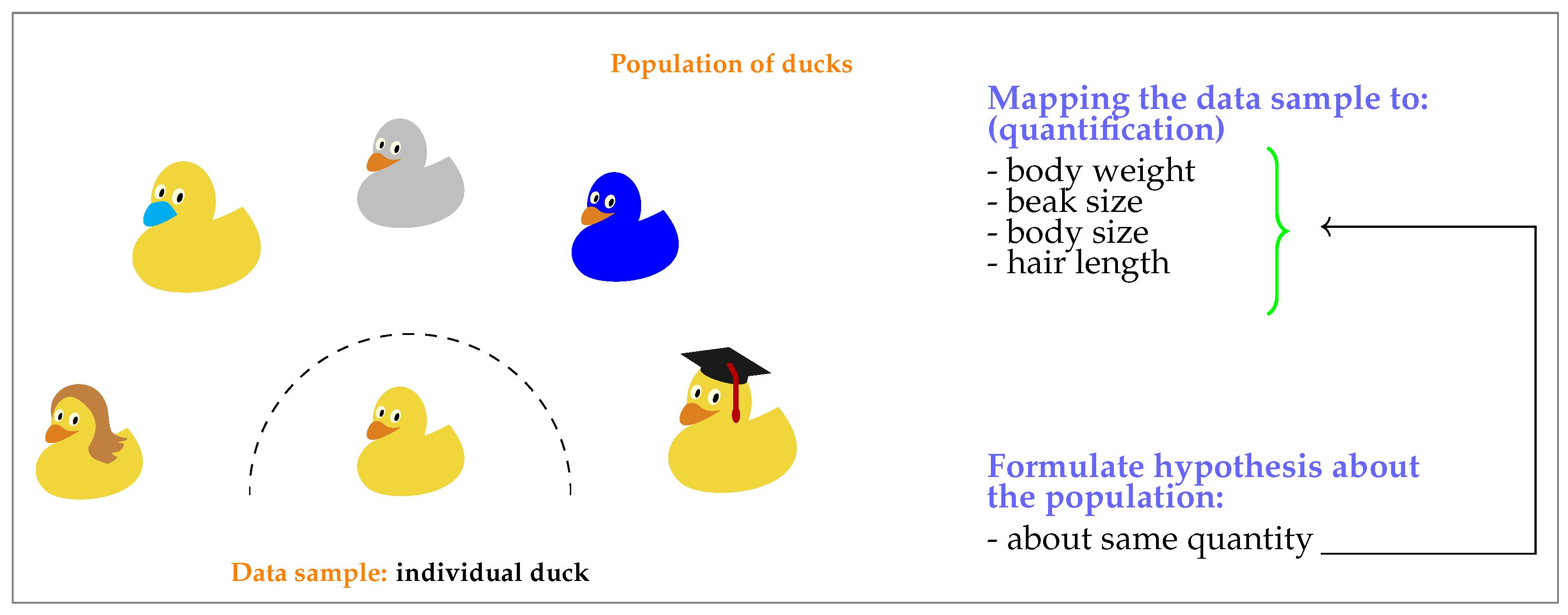
The principle idea of a statistical hypothesis test is to decide if a data sample is typical or atypical compared to a population assuming a hypothesis we formulated about the population is true. Here a data sample refers to a small portion of entities taken from a population, for example, via an experiment, whereas the population comprises all possible entities.
In Figure 1 we give an intuitive example for the basic idea of hypothesis testing. In this particular example the population consists of all ducks and the data sample is one individual duck randomly drawn from the entire population. In statistics ‘randomly drawn’ is referred to as ‘sampling’. In order to perform the comparison between the data sample and the population one needs to introduce a quantification of the situation. In our case this quantification consists in a mapping from a duck to a number. This number could correspond to, for example, the body weight, the beak size, the body size or the hair length of a duck. In statistics this mapping is called test statistic.
A key component in hypothesis testing is of course a ‘hypothesis’. The hypothesis is a quantitative statement we formulate about the population value of the test statistic. In our case it could be about the body parts of a duck, for example, body size. A particular hypothesis we can formulate is: The mean body size equals 20 cm. Such a hypothesis is called the null hypothesis .
Assuming now we are having a population of ducks having a body size of 20 cm including natural variations. Due to the fact that the population consists of (infinite) many ducks and for each we are obtaining such a quantification this results in a probability distribution, called the sampling distribution, for the mean body size. Here it is important to note that our population is a hypothetical population which obeys our null hypothesis. In other words, the null hypothesis specifies the population completely.
Having now a numerical value of the test statistic, representing the data sample and the sampling distribution, representing the population, we can compare both with each other in order to evaluate the null hypothesis that we have formulated. From this comparison we obtain another numerical value, called the p-values, which quantifies the typicality or atypicality of the configuration assuming the null hypothesis is true. Finally, based on the p-values a decision is made.
On a technical note, we want to remark that due to the fact that in the above problem there is only one population involved this is called an one-sample hypothesis test. However, the principal idea extends also to hypothesis tests involving more than population.
3. Key Components of Hypothesis Testing
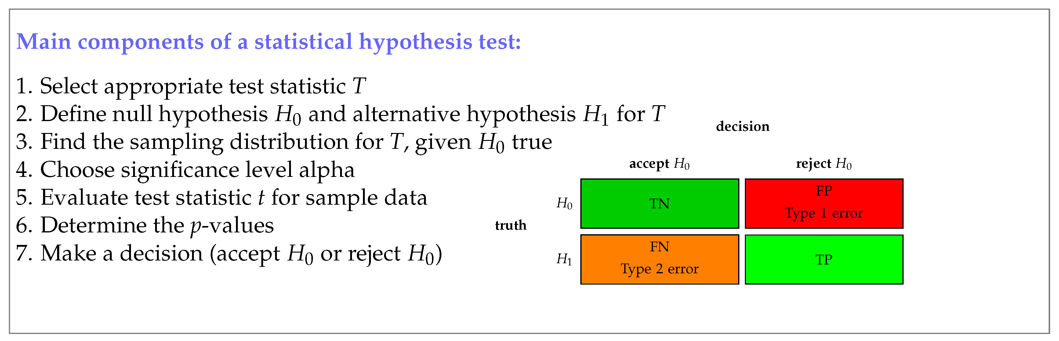
In the following sections, we will formalize the example discussed above. In general, regardless of the specific hypothesis test one is conducting, there are seven components common to all hypothesis tests. These components are summarized in Figure 2. We listed these components in the order they are entering the process when performing a hypothesis test. For this reason they can be also considered as steps of a hypothesis test. Due to the fact that they are interconnected with each other their logical order is important. Overall this means a hypothesis test is a procedure that needs to be executed. In the following subsections, we will discuss each of these seven procedural components in detail.
3.1. Step 1: Select Test Statistic
Put simply, a test statistic quantifies a data sample. In statistics the term ‘statistic’ refers to any mapping (or function) between a data sample and a numerical value. Popular examples are the mean value or the variance. Formally, the test statistic can be written as
whereas is a data sample with sample size n. Here we denoted the mapping by T and the value we obtain by . Typically the test statistic can assume real values, that is, but restrictions are possible.
A test statistic assumes a central role in a hypothesis test because by deciding which test statistic to use one determines a hypothesis test to a large extend. The reason is that it will enter the hypotheses we formulate in step 2. For this reason one needs to carefully select a test statistic that is of interest and importance for the conducted study.
We would like to emphasize that in this step, we select the test statistics but we neither evaluate it nor we use it yet. This is done in step 5.
3.2. Step 2: Null Hypothesis and Alternative Hypothesis
At this step, we define two hypotheses which are called the null hypothesis and the alternative hypothesis . Both hypotheses make statements about the population value of the test statistic and are mutually exclusive. For the test statistic we selected in step 1, we call the population value of t as . Based on this we can formulate the following hypotheses:
- null hypothesis: :
- alternative hypothesis: :
As one can see, the way the two hypotheses are formulated, the value of the population parameter can only be true for one statement but not for both. For instance, either is true but then the alternative hypothesis is false or is true but then the null hypothesis is false.
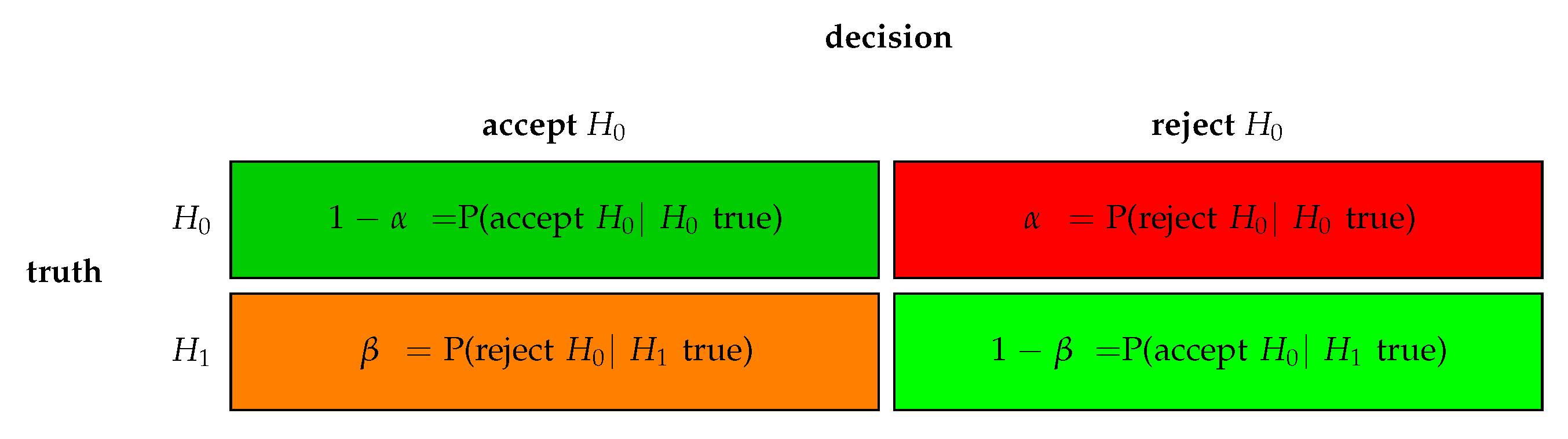
In Figure 2, we show the four possible outcomes of a hypothesis test. Each of these outcomes has a specific name that is commonly used. For instance, if the null hypothesis is false and we reject this is called a ‘true positive’ (TP) decision. The reason for calling it ‘positive’ is related to the asymmetric meaning of a hypothesis test, because rejecting when is false is more informative than accepting when is true. In this case one can consider the outcome of a hypothesis test a positive result.
The alternative hypothesis formulated above is an examples for a one-side hypothesis. Specifically, we formulated a right-sided hypothesis because the alternative assumes values larger than . In addition, we can formulate a left-sided alternative hypothesis stating
- alternative hypothesis: :
Furthermore, we can formulate a two-side alternative hypothesis that is indifferent regarding the side by
- alternative hypothesis: :
Despite the fact that there are hundreds of different hypothesis tests [26], the above description principally holds for all of them. However, this does not mean that if you understand one hypothesis test you understand all but if you understand the principle of one hypothesis test you understand the principle of all.
In order to connect the test statistic t, which is a sample value, with its population value one needs to know the probability distribution of the test statistic. Because of this connection, this probability distribution received a special name and is called the sampling distribution of the test statistic. It is important to emphasize that the sampling distribution represents the values of the test statistic assuming the null hypothesis is true. This means that in this case the population value of is .
Let’s assume for now that we know the sampling distribution for our test statistic. By comparing the particular value t of our test statistic with the sampling distribution in a way that is determined by the way we formulated the null and the alternative hypothesis, we obtain a quantification for the ‘typicality’ of this value with respect to the sampling distribution, assuming the null hypothesis is true.
3.3. Step 3: Sampling Distribution
In our general discussion about the principle idea of a hypothesis test above, we mentioned that the connection between a test statistic and its sampling distribution is crucial for any hypothesis test. For this reason, we elaborate in this section on this point in more detail.
In this section, we want to answer the following questions:
- What is the sampling distribution?
- How to obtain the sampling distribution?
- How to use the sampling distribution?
To 1.: First of all, the sampling distribution is a probability distribution. The meaning of this sampling distribution is that it is the distribution of the test statistic T, which is a random variable, given some assumptions. We can make this statement more precise by defining the sampling distribution of the null hypothesis as follows.
Definition 1.
Let be a random sample from a population with and be a test statistic. Then the probability distribution of , assuming is true, is called the sampling distribution of the null hypothesis or the null distribution.
Similarly, one defines the sampling distribution of the alternative hypothesis by . Since there are only two different hypotheses, and , there are only two different sampling distributions in this context. However, we would like to note that sampling distributions are also playing a role outside statistical hypothesis testing, for example, for estimation theory or data Bootstrapping [27].
There are several points in the above definition we would like to highlight. First, the distribution from which the random variables are sampled can assume any form and is not limited to, for example, a normal distribution. Second, the test statistic is a random variable itself because it is a function of random variables. For this reason there exists a distribution that belongs to this random variable in a way that the values of this random variable are samples thereof. Third, the test statistic is a function of the sample size n and for this reason also the sampling distribution is a function of n. That means, if we change the sample size n, we change the sampling distribution. Fourth, the fact that is the probability distribution of means that by taking infinite many samples from in the form, , we can perfectly reconstruct the distribution itself. The last point allows under certain conditions a numerical approximation of the sampling distribution, as we will see in the following example.
Examples
Suppose we have a random sample of size n whereas each data point is sampled from a gamma distribution with and , that is, . Furthermore, let’s use the mean value as a test statistic, that is,
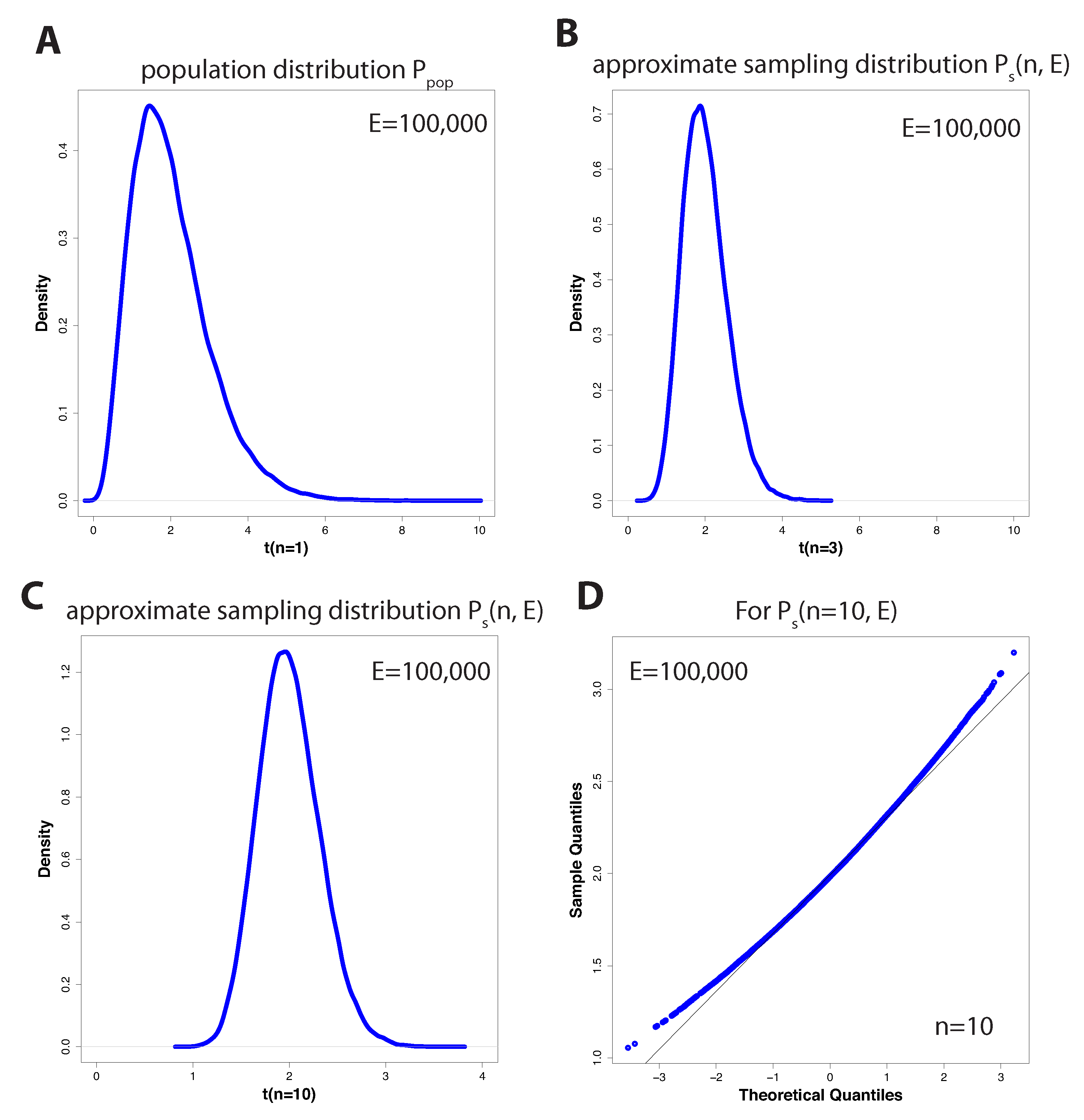
In Figure 3A–C, we show three examples for three different values of n (in A , in B and in C ) when drawing E = 100,000 samples , from which we estimate E = 100,000 different mean values T. Specifically, in Figure 3A–C we show density estimates of these 100,000 values. As indicated above, in the limit of infinite many samples E, the approximate sampling distribution will become the (theoretical) sampling distribution, that is,
as a function of the sample size n.
For , we obtain the special case that the sampling distribution is the same as the underlying distribution of the population , which is in our case a gamma distribution with the parameters and , shown in Figure 3A. For all other , we observe a transformation in the distributional shape of the sampling distribution, as seen in Figure 3B,C. However, this transformation should be familiar to us because from the Central Limit Theorem we know that the mean of independent samples with mean and variance follows a normal distribution with mean and standard deviation , that is,
We notice that this result is only strictly true in the limit of large n. However, in Figure 3D, we show a qq-plot that demonstrates that already for the resulting distribution, = 100,000), is quite close to such a normal distribution (with the appropriate parameters).
We would like to remind that the Central Limit Theorem holds for arbitrarily iid (independent and identically distributed) random variables . Hence, the sampling distribution for the mean is always the normal distribution given in Equation (4).
There is one further simplification we obtain by applying a so called z-transformation of the mean value of to Z by
because the distribution of Z is a standard normal distribution, that is,
Now, we reached an important point where we need to ask ourself if we are done. This depends on our knowledge about the variance. If we know the variance the sampling distribution of our transformed mean , we called Z, is a standard normal distribution. However, if we do not know the variance , we cannot perform the z-transformation in Equation (5), because this transformation depends on . In this case, we need to estimate the variance of the random sample by
Then we can use the estimate for the variance to use it for the following t-transformation
Despite the fact that this t-transformation is formally similar to the z-transformation in Equation (5) the resulting random variable T does not follow a standard normal distribution but a Students’ t-distribution with degrees of freedom (dof). We want to mention that this holds strictly for , that is, normal distributed samples.
3.4. Step 4: Significance Level
The significance level is a number between zero and one, that is, . It has the meaning
giving the probability to reject provided is true. That means it gives us the probability of making a Type 1 error resulting in a false positive decision.
When conducting a hypothesis test, we have the freedom to choose this value. However, when deciding about its numerical value one needs to be aware of potential consequences. Possibly the most frequent choice of is , however, for Genome-Wide Association Studies (GWAS) values as low as are used [28]. The reason for such a wide variety of used values is in the possible consequences in the different application domains. For GWAS, Type 1 errors can result in wasting millions of Dollars because follow-up experiments in this field are very costly. Hence, is chosen very small.
3.5. Step 5: Evaluate Test Statistic from Data
This step is our connection to the real world, as represented by the data, because everything until here has been theoretical. For we estimate the numerical value of the test statistic selected in Step 1 giving
Here represents a particular numerical value obtained from the observed data . Due to the fact that our data set depends on the number of samples n, also this numerical value will be dependent on n. This is explicitly indicated by the subscript.
3.6. Step 6: Determine the p-Values
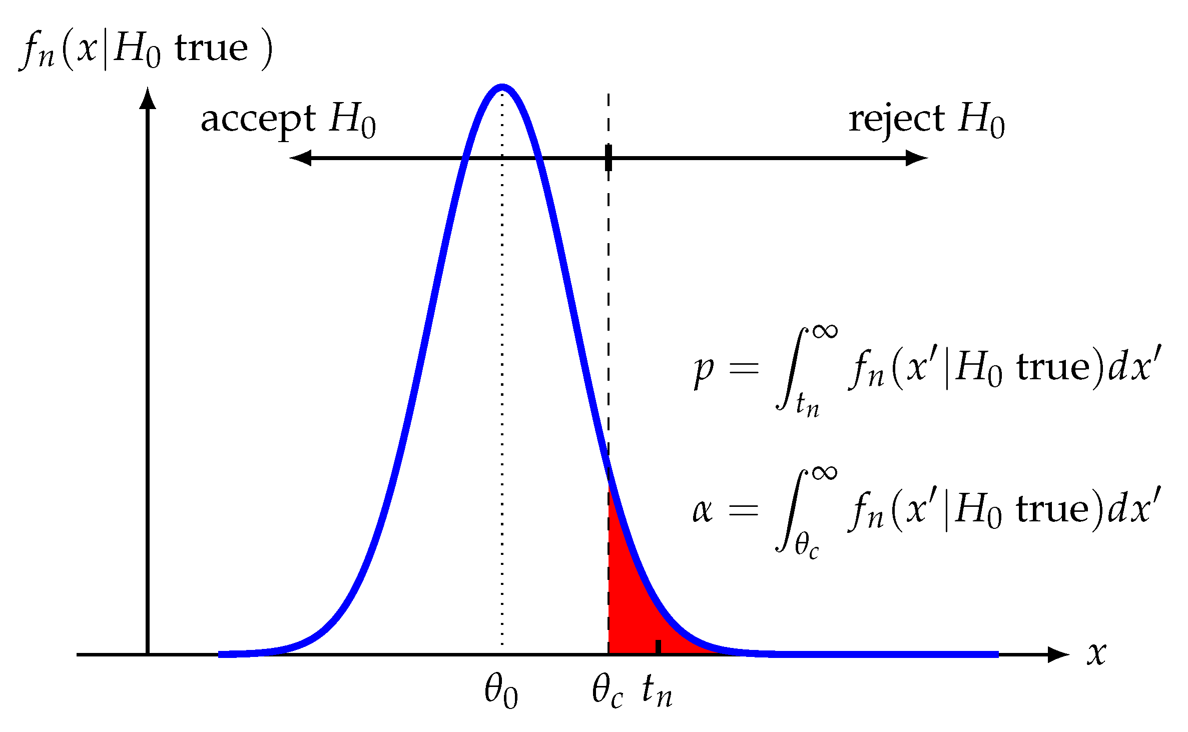
For determining the p-values of a hypothesis test, we need to use the sampling distribution (Step 3) and the estimated test statistic (Step 5). That means the p-values results from a comparison of theoretical assumptions (sampling distribution) with real observations (data sample) assuming is true. This situation is visualized in Figure 4 for a right-sided alternative hypothesis. The p-values is the probability for observing more extreme values than the test statistic assuming is true
Formally it is obtained by an integral over the sampling distribution
The final decision if we reject or accept the null hypothesis will be based on the numerical value of p.
Furthermore, we can use the following integral
to solve for . That means, the significance level implies a threshold . This threshold can also be used to make a decision about .
We would like to emphasize that due to the fact that the test statistic is a random variable also the p-values is a random variable since it depends on the test statistic [29].
Remark 1.
The sample size n has an influence on the numerical analysis of the problem. For this reason the test statistic and the sampling distribution are indexed by it. However, it has no effect on the formulation and expression of the hypothesis because we make statements about a population value that hold for all n.
3.7. Step 7: Make a Decision about the Null Hypothesis
In the final step we are making a decision about the null hypothesis. In order to do this there are two alternative ways. First, we can make a decision based on the p-values or, second, we make a decision based on the value of the test statistic .
- Decision based on the p-values:
- Decision based on the threshold :
In case we cannot reject the null hypothesis we accept it.
4. Type 2 Error and Power
When making binary decisions there is a number of errors one can make [30]. In this section, we go one step back and take a more theoretical look on a hypothesis test with respect to the possible errors one can make. In section ‘Step 2: Null hypothesis and alternative hypothesis ′ we discussed that there are two possible errors one can make, a false positive and a false negative and when discussing Step 4, we introduced formally the meaning of a Type 1 error. Now we extend this discussion to the Type 2 error.
As mentioned previously, there are only two possible configurations one needs to distinguish. Either is true or it is false. If is true (false) it is equally correct to say is false (true). Now, let’s assume is true. For evaluating the Type 2 error we require the sampling distribution assuming is true. However, for performing a hypothesis test, as discussed in the previous sections (see Figure 2), we do not need to know the sampling distribution assuming is true. Instead, we need to know the sampling distribution assuming is true because this distribution corresponds to the null hypothesis. The good news is the sampling distribution assuming is true can be easily obtained if we make the alternative hypothesis more precise. Let’s assume we are testing the following hypothesis.
- null hypothesis: :
- alternative hypothesis: :
In this case is precisely specified because it sets the population parameter to . In contrast, limits the range of possible values for but does not set it to a particular value.
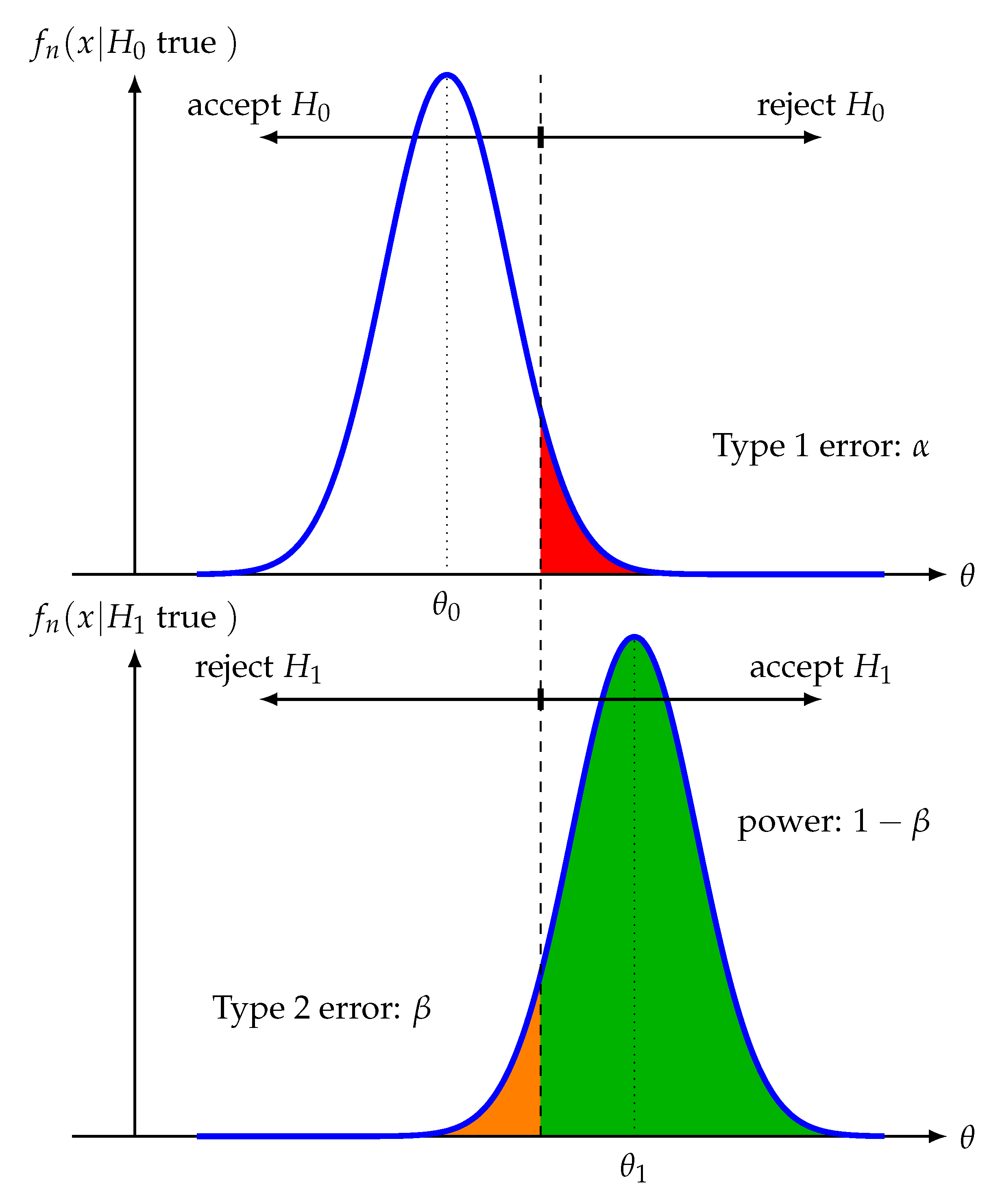
For determining the Type 2 error we need to set in the alternative hypothesis to a particular value. So let’s set the population parameter in for . In Figure 5 we visualize the sampling distribution for and .
If we reject when is true, this is a correct decision and the green area in Figure 5 represents the corresponding probability for this, formally given by
For short this probability is usually denoted by and called the power of a test.
On the other hand, if we do not reject when is true, we make an error, given by
This is called a Type 2 error. In Figure 5, we highlight the Type 2 error probability in orange.
We would like to emphasize that the Type 1 error and the Type 2 error are both long-run frequencies for repeated experiments. That means both probabilities give the error when repeating the exact same test many times. This is in contrast to the p-values, which is the probability for a given data sample. Hence, the p-values does not allow to draw conclusions for repeated experiments.
Connections between Power and Errors
From Figure 5 we can see the relation between power (), Type 1 error () and Type 2 error (), summarized in Figure 6. Ideally, one would like to have a test with a high power and low Type 1 error and low Type 2 error. However, from Figure 5 we see that these three entities are not independent from each other. Specifically, if we increase the power () by changing we increase the Type 1 error () because this will reduce the critical value . In contrast, reducing leads to an increase in Type 2 error () and a reduction in power. Hence, in practice, one needs to make a compromise between the ideal goals.
For the discussion above, we assumed a fixed sample size n. However, as we discussed in the example of section ‘Step 3: Sampling distribution’, the variance of the sampling distribution depends on the sample size via the standard error in the way
This opens another way to increase the power and to minimize the Type 2 error by increasing the sample size n. By keeping the population means and unchanged but increasing the sample size to a value larger than n, that is, , the sampling distributions for and become narrower because their variances decrease according to Equation (18). Hence, as a consequence of an increased sample size the overlap between the distributions, as measured by , is reduced leading to an increase in the power and a decrease in Type 2 error for an unchanged value of the significance level . In the extreme case for the power approaches 1 and the Type 2 error 0, for a fixed Type 1 error .
From this discussion the importance of the sample size in a study becomes apparent as a control mechanism to influence the resulting power and the Type 2 error.
5. Confidence Intervals
The test statistic is a function of the data (see Step 1 in Section 3.1) and, hence, it is a random variable. That means there is a variability of a test statistic because its value changes for different samples. In order to quantify the interval within which such values fall, one uses a confidence interval (CI) [31,32].
Definition 2.
The interval is called a confidence interval for parameter θ if it contains this parameter with probability for , that is,
The interpretation of a CI is that for repeated samples the confidence intervals of these are expected to contain the true with probability . Here it is important to note that is fixed because it is a population value. What is random is the estimate of the boundaries of the CI, that is, a and b. Hence, for repeated samples, is fixed but I is a random interval.
The connection between a confidence interval and a hypothesis test for a significance level of is that if the value of the test statistic falls within the CI then we do not reject the null hypothesis. On the other hand, if the confidence interval does not contain the value of the test statistic, we reject the null hypothesis. Hence, the decisions reached by both approaches agree always with each other.
If one does not make any assumption about the shape of the probability distribution, for example, symmetry around zero, there are infinite many CIs because neither the starting nor the ending values of a and b are uniquely defined but follow from assumptions. Frequently, one is interested in obtaining a CI for a quantile separation of the data in the form
whereas and are quantiles of the sampling distribution with respect to respectively of the data.
5.1. Confidence Intervals for a Population Mean with Known Variance
From the central limit theorem we know that the sum of random variables is normal distributed. If we normalize this by
then Z follows a standard normal distribution, that is, , whereas is the standard error
of .
Here the values of are obtained by solving the equations for a standard normal distributed probability
Using these and solving the inequality in Equation (23) for the expectation value gives the confidence interval with
Here we assumed that is know. Hence, the above CI is valid for a z-test.
5.2. Confidence Intervals for a Population Mean with Unknown Variance
If we assume that is not know then the sampling distribution of a population mean is Student’s T-distribution and needs to be estimated from samples by the sample standard deviation s. In this case a similar derivation as above results in
Here are critical values for a Student’s T-distribution, obtained similarly as in Equations (26) and (27). Such a CI is valid for a t-test.
5.3. Bootstrap Confidence Intervals
In case a sampling distribution is not given in analytical form numerical approaches need to be used. In such a situation a CI can be numerically obtained via nonparametric Bootstrap [33]. This is the most generic way to obtain a CI. By utilizing the augmented definition in Equation (20) for any test statistic the CI can be obtained from
whereas the quantiles and are directly obtained from the data resulting in . Such a confidence interval can be used for any statistical hypothesis test.
We would like to emphasize that in contrast to Equation (20) here the quantiles and are estimates of the quantiles and from the sampling distribution. Hence, the obtained CI is merely an approximation.
6. An Example and a Warning
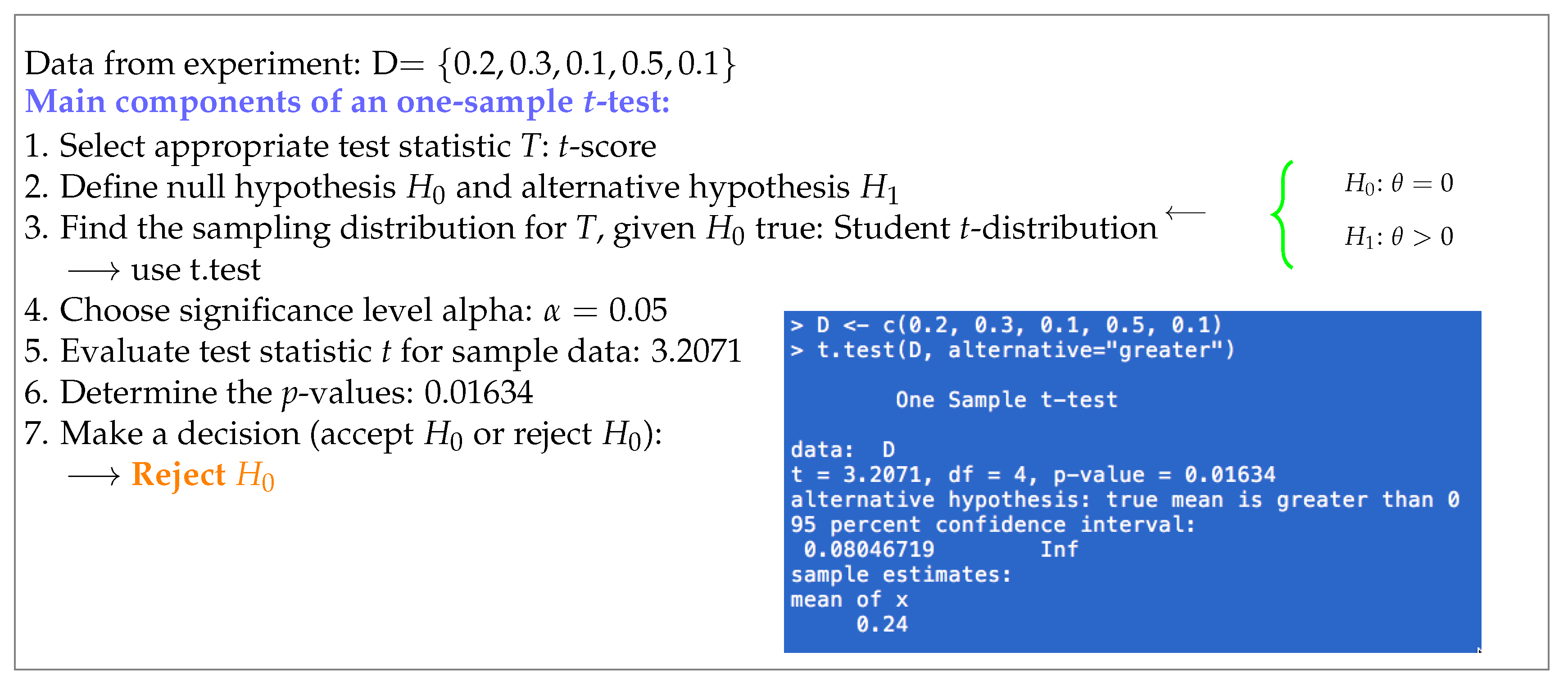
Finally, we are providing a practical example for an one-sample t-test that will also serve as a warning. In Figure 7 we show a worked example for a data set D defining the major components of a t-test.
On the left-hand side of Figure 7 a summary of the test is presented and on the right-hand side of Figure 7 we show a script in the programming language R providing the numerical solution to the problem. R is a widespreadly used programming language to study statistical problems [34]. The solution script is only two lines, in the first the data sample is defined and in the second the hypothesis test is conducted. The command ‘t.test’ has arguments that specify the used data and the type of the alternative hypothesis. In our case we are using a right-sided alternative indicated by ‘greater’. In addition, the null hypothesis needs to be specified. In our case we used the default which is , however, by using the argument ‘mu’ one can set different values.
From this example one can learn the following. First, the practical execution of a hypothesis test with a computer is very simple. In fact, every hypothesis test assumes a similar form as the provided example. Second, due to the simplicity, all complexity of a hypothesis test, as discussed in the previous sections of this paper, is hidden behind the abstract computer command ‘t.test’. However, from this follows that a deeper understanding of a hypothesis test cannot be obtained by the practical execution of problems if cast into a black-box frame (in the above example ‘t.test’ is the black-box). The last point maybe counterintuitive if one skips the above discussion, however, we consider this one cause for the widespread misunderstanding of statistical hypothesis tests in general.
7. Historical Notes and Misinterpretations
The modern formulation of statistical hypothesis testing, as discussed in this paper, has not been introduced as one theory but it evolved from two separately introduced theories and accompanied concepts. The first method is due to Fisher [4] and the second due to Neyman and Pearson [8]. Since about the 1960s an unified form was established (some call this null hypothesis significance testing (NHST)) in the literature as it is used to date [35,36].
Briefly, Fisher introduced the concept of a p-values while Neyman and Pearson introduced the alternative hypothesis as complement to the null hypothesis, type I and type II errors and the power. There is an ongoing discussion about the differences of both concepts see, for example, References [37,38,39], which is in general very difficult to follow because these involve also philosophical interpretations of those theories. Unfortunately, these differences are not only of interest for historical reasons but lead to contaminations and misunderstandings of the modern formulation of statistical hypothesis testing because often arguments are taken out of context and properties differ among the different theories [40,41]. For this reason, we discuss some of those in the following.
- Is the p-values the probability that the null hypothesis is true given the data?No, it is the probability of observing more extreme values than the test statistic, if the null hypothesis is true, that is, see Equation (11). Hence, one assumes already that is true for obtaining the p-values. Instead, the question aims to find .
- Is the p-values the probability that the alternative hypothesis is true given the data?No, see question (1). This would be .
- If the null hypothesis is rejected, is the p-values the probability of your rejection error?No, the rejection error is the type I error given by .
- Is the p-values the probability to observe our data sample given the null hypothesis is true?No, this would be the Likelihood.
- If one repeats an experiments does one obtain the same p-values?No, because p-valuess do not provide information about the long run frequencies of repeated experiments as the type I or type II errors. Instead, they give the probability resulting from comparing the test statistic (as a function of the data) and the null hypothesis assumed to be true.
- Does the p-values give the probability that the data were produced by random chance alone?No, despite the fact that the data were produced by assuming it is true. The p-values does not provide the probability for this.
- Does the same p-values from two studies provide the same evidence against the null hypothesis?Yes, but only in the very rare case if everything in the two studies and the formulated hypotheses is identical. This includes also the sample sizes. In any other case, p-valuess are difficult to compare with each other and no conclusion can be drawn.
We think that many of the above confusions are a result from verbal interpretations of the theory by neglecting mathematical definitions of used entities. This is understandable since many people interested in the application of statistical hypothesis testing have not received formal training in the underlying probability theory. A related problem is that a hypothesis test is exactly set-up to answer one question and that is based on a data sample to reject a null hypothesis or not. There are certainly many more questions experimentalists would like to have answers for, however, a statistical hypothesis test is not designed for these. It is only possible to derive some related answers to questions that are closely related to the set-up of the hypothesis test. For this reason in general it is a good strategy to start answering any question in the context of statistical hypothesis testing by looking at the basic definition of the involved entities because only these are exact and provide unaltered interpretations.
8. The Future of Statistical Hypothesis Testing
Despite the fact that the core methodology of statistical hypothesis testing is dating back many decades questions regarding its interpretation and practical usage are to date under discussion [42,43,44,45,46]. This is due to the involvedness and complexity of the methodology demanding a thorough education because otherwise problems are implicated [47] and even unsound designs may be overlooked [12]. Furthermore, there are constantly new statistical hypothesis tests being developed that built upon the standard methodology, for example, by using novel test statistics [48,49,50]. Given the need to make sense of the increasing flood of data, we are currently facing in all areas of science and industry, statistical hypothesis testing provides a tool for binary decision making. Hence, it allows to convert data into decisions. Due to the need for scientific decision making a future without statistical hypothesis testing is hard to imagine.
9. Conclusions
In this paper we provided a primer on statistical hypothesis testing. Due to the difficulty of the problem, we were aiming at an accessible level of description and presented the bare backbone of the method. We avoided application domain specific formulations in order to make the knowledge transfer easier to different application areas in data science including biomedical science, economics, management, politics, marketing, medicine, psychology or social science [50,51,52,53,54,55].
Finally, we would like to note that in many practical applications one does not perform one but multiple hypothesis tests simultaneously. For instance, for identifying the differential expression of genes or the significant change of stock prices. In such a situation one needs to apply a multiple testing correction (MTC) for controlling the resulting errors [56,57,58,59]. This is a highly non-trivial and a complex topic for itself that can lead to erroneous outcomes if not properly addressed [60].
Author Contributions
F.E.-S. conceived the study. All authors contributed to the writing of the manuscript and approved the final version.
Funding
M.D. thanks the Austrian Science Funds for supporting this work (project P30031).
Conflicts of Interest
The authors declare no conflict of interest. The founding sponsors had no role in the design of the study; in the collection, analyses, or interpretation of data; in the writing of the manuscript, and in the decision to publish the results.
References
- Helbing, D. The Automation of Society Is Next: How to Survive the Digital Revolution. 2015. Available online: https://ssrn.com/abstract=2694312 (accessed on 1 June 2019).
- Hacking, I. Logic of Statistical Inference; Cambridge University Press: Cambridge, UK, 2016. [Google Scholar]
- Gigerenzer, G. The Superego, the Ego, and the id in Statistical Reasoning. In A Handbook for Data Analysis in the Behavioral Sciences: Methodological Issues; Lawrence Erlbaum Associates, Inc.: Mahwah, NJ, USA, 1993; pp. 311–339. [Google Scholar]
- Fisher, R.A. Statistical Methods for Research Workers; Genesis Publishing Pvt Ltd.: Guildford, UK, 1925. [Google Scholar]
- Fisher, R.A. The Arrangement of Field Experiments (1926). In Breakthroughs in Statistics; Springer: Berlin, Germany, 1992; pp. 82–91. [Google Scholar]
- Fisher, R.A. The statistical method in psychical research. Proc. Soc. Psych. Res. 1929, 39, 189–192. [Google Scholar]
- Neyman, J.; Pearson, E.S. On the use and interpretation of certain test criteria for purposes of statistical inference: Part I. Biometrika 1967, 20, 1–2. [Google Scholar]
- Neyman, J.; Pearson, E.S. On the Problem of the Most Efficient Tests of Statistical Hypotheses. Philos. Trans. R. Soc. Lond. 1933, 231, 289–337. [Google Scholar] [CrossRef]
- Lehman, E. Testing Statistical Hypotheses; Springer: New York, NY, USA, 2005. [Google Scholar]
- Dudoit, S.; Shaffer, J.; Boldrick, J. Multiple hypothesis testing in microarray experiments. Stat. Sci. 2003, 18, 71–103. [Google Scholar] [CrossRef]
- Tripathi, S.; Emmert-Streib, F. Assessment Method for a Power Analysis to Identify Differentially Expressed Pathways. PLoS ONE 2012, 7, e37510. [Google Scholar] [CrossRef] [PubMed]
- Tripathi, S.; Glazko, G.; Emmert-Streib, F. Ensuring the statistical soundness of competitive gene set approaches: Gene filtering and genome-scale coverage are essential. Nucleic Acids Res. 2013, 6, e53354. [Google Scholar] [CrossRef] [PubMed]
- Jiang, Z.; Gentleman, R. Extensions to gene set enrichment. Bioinformatics 2007, 23, 306–313. [Google Scholar] [CrossRef] [PubMed]
- Emmert-Streib, F. The Chronic Fatigue Syndrome: A Comparative Pathway Analysis. J. Comput. Biol. 2007, 14, 961–972. [Google Scholar] [CrossRef]
- Siroker, D.; Koomen, P. A/B Testing: The Most Powerful Way to Turn Clicks into Customers; John Wiley & Sons: Hoboken, NJ, USA, 2013. [Google Scholar]
- Mauri, L.; Hsieh, W.h.; Massaro, J.M.; Ho, K.K.; D’agostino, R.; Cutlip, D.E. Stent thrombosis in randomized clinical trials of drug-eluting stents. N. Engl. J. Med. 2007, 356, 1020–1029. [Google Scholar] [CrossRef] [PubMed]
- Deuschl, G.; Schade-Brittinger, C.; Krack, P.; Volkmann, J.; Schäfer, H.; Bötzel, K.; Daniels, C.; Deutschländer, A.; Dillmann, U.; Eisner, W.; et al. A randomized trial of deep-brain stimulation for Parkinson’s disease. N. Engl. J. Med. 2006, 355, 896–908. [Google Scholar] [CrossRef] [PubMed]
- Molina, I.; Gómez i Prat, J.; Salvador, F.; Treviño, B.; Sulleiro, E.; Serre, N.; Pou, D.; Roure, S.; Cabezos, J.; Valerio, L.; et al. Randomized trial of posaconazole and benznidazole for chronic Chagas’ disease. N. Engl. J. Med. 2014, 370, 1899–1908. [Google Scholar] [CrossRef] [PubMed]
- Shoptaw, S.; Yang, X.; Rotheram-Fuller, E.J.; Hsieh, Y.C.M.; Kintaudi, P.C.; Charuvastra, V.; Ling, W. Randomized placebo-controlled trial of baclofen for cocaine dependence: Preliminary effects for individuals with chronic patterns of cocaine use. J. Clin. Psychiatry 2003, 64, 1440–1448. [Google Scholar] [CrossRef] [PubMed]
- Sedlmeier, P.; Eberth, J.; Schwarz, M.; Zimmermann, D.; Haarig, F.; Jaeger, S.; Kunze, S. The psychological effects of meditation: A meta-analysis. Psychol. Bull. 2012, 138, 1139. [Google Scholar] [CrossRef] [PubMed]
- Casscells, W.; Schoenberger, A.; Graboys, T.B. Interpretation by Physicians of Clinical Laboratory Results. N. Engl. J. Med. 1978, 299, 999–1001. [Google Scholar] [CrossRef] [PubMed]
- Ioannidis, J.P.A. Why Most Published Research Findings Are False. PLoS Med. 2005, 2. [Google Scholar] [CrossRef] [PubMed]
- Banerjee, I.; Bhadury, T. Self-medication practice among undergraduate medical students in a tertiary care medical college, West Bengal. Ind. Psychiatry J. 2009, 18, 127–131. [Google Scholar] [CrossRef]
- Taroni, F.; Biedermann, A.; Bozza, S. Statistical hypothesis testing and common misinterpretations: Should we abandon p-values in forensic science applications? Forensic Sci. Int. 2016, 259, e32–e36. [Google Scholar] [CrossRef]
- Emmert-Streib, F.; Dehmer, M. Defining Data Science by a Data-Driven Quantification of the Community. Mach. Learn. Knowl. Extr. 2019, 1, 235–251. [Google Scholar] [CrossRef]
- Sheskin, D.J. Handbook of Parametric and Nonparametric Statistical Procedures, 3rd ed.; RC Press: Boca Raton, FL, USA, 2004. [Google Scholar]
- Chernick, M.R.; LaBudde, R.A. An Introduction to Bootstrap Methods with Applications to R; John Wiley & Sons: Hoboken, NJ, USA, 2014. [Google Scholar]
- Panagiotou, O.A.; Ioannidis, J.P.; Project, G.W.S. What should the genome-wide significance threshold be? Empirical replication of borderline genetic associations. Int. J. Epidemiol. 2011, 41, 273–286. [Google Scholar] [CrossRef]
- Murdoch, D.J.; Tsai, Y.L.; Adcock, J. p-valuess are random variables. Am. Stat. 2008, 62, 242–245. [Google Scholar] [CrossRef]
- Emmert-Streib, F.; Moutari, S.; Dehmer, M. A comprehensive survey of error measures for evaluating binary decision making in data science. Wiley Interdiscip. Rev. Data Min. Knowl. Discov. 2019, e1303. [Google Scholar] [CrossRef]
- Breiman, L. Statistics: With a View Toward Applications; Houghton Mifflin Co.: Boston, MA, USA, 1973. [Google Scholar]
- Baron, M. Probability and Statistics for Computer Scientists; Chapman and Hall/CRC: New York, NY, USA, 2013. [Google Scholar]
- Efron, B.; Tibshirani, R. An Introduction to the Bootstrap; Chapman and Hall/CRC: New York, NY, USA, 1994. [Google Scholar]
- R Development Core Team. R: A Language and Environment for Statistical Computing; R Foundation for Statistical Computing: Vienna, Austria, 2008; ISBN 3-900051-07-0. [Google Scholar]
- Nix, T.W.; Barnette, J.J. The data analysis dilemma: Ban or abandon. A review of null hypothesis significance testing. Res. Sch. 1998, 5, 3–14. [Google Scholar]
- Szucs, D.; Ioannidis, J. When null hypothesis significance testing is unsuitable for research: A reassessment. Front. Hum. Neurosci. 2017, 11, 390. [Google Scholar] [CrossRef] [PubMed]
- Biau, D.J.; Jolles, B.M.; Porcher, R. P value and the theory of hypothesis testing: An explanation for new researchers. Clin. Orthop. Relat. Res.® 2010, 468, 885–892. [Google Scholar] [CrossRef] [PubMed]
- Lehmann, E.L. The Fisher, Neyman-Pearson theories of testing hypotheses: One theory or two? J. Am. stat. Assoc. 1993, 88, 1242–1249. [Google Scholar] [CrossRef]
- Perezgonzalez, J.D. Fisher, Neyman-Pearson or NHST? A tutorial for teaching data testing. Front. Psychol. 2015, 6, 223. [Google Scholar] [CrossRef] [PubMed]
- Greenland, S.; Senn, S.J.; Rothman, K.J.; Carlin, J.B.; Poole, C.; Goodman, S.N.; Altman, D.G. Statistical tests, P values, confidence intervals, and power: A guide to misinterpretations. Eur. J. Epidemiol. 2016, 31, 337–350. [Google Scholar] [CrossRef]
- Goodman, S. A Dirty Dozen: Twelve p-values Misconceptions. In Seminars in Hematology; Elsevier: Amsterdam, The Netherlands, 2008; Volume 45, pp. 135–140. [Google Scholar]
- Wasserstein, R.L.; Lazar, N.A. The ASA’s statement on p-valuess: Context, process, and purpose. Am. Stat. 2016, 70, 129–133. [Google Scholar] [CrossRef]
- Wasserstein, R.L.; Schirm, A.L.; Lazar, N.A. Moving to a World Beyond p < 0.05. Am. Stat. 2019, 73, 1–19. [Google Scholar] [CrossRef]
- Ioannidis, J. Retiring significance: A free pass to bias. Nature 2019, 567, 461. [Google Scholar] [CrossRef]
- Amrhein, V.; Greenland, S.; McShane, B. Scientists rise up against statistical significance. Nature 2019, 567, 305. [Google Scholar] [CrossRef]
- Benjamin, D.J.; Berger, J.O. Three Recommendations for Improving the Use of p-valuess. Am. Stat. 2019, 73, 186–191. [Google Scholar] [CrossRef]
- Gigerenzer, G.; Gaissmaier, W.; Kurz-Milcke, E.; Schwartz, L.M.; Woloshin, S. Helping doctors and patients make sense of health statistics. Psychol. Sci. Public Interest 2007, 8, 53–96. [Google Scholar] [CrossRef] [PubMed]
- Rahmatallah, Y.; Emmert-Streib, F.; Glazko, G. Gene Sets Net Correlations Analysis (GSNCA): A multivariate differential coexpression test for gene sets. Bioinformatics 2014, 30, 360–368. [Google Scholar] [CrossRef] [PubMed]
- De Matos Simoes, R.; Emmert-Streib, F. Bagging statistical network inference from large-scale gene expression data. PLoS ONE 2012, 7, e33624. [Google Scholar] [CrossRef] [PubMed]
- Rahmatallah, Y.; Zybailov, B.; Emmert-Streib, F.; Glazko, G. GSAR: Bioconductor package for Gene Set analysis in R. BMC Bioinform. 2017, 18, 61. [Google Scholar] [CrossRef]
- Cortina, J.M.; Dunlap, W.P. On the logic and purpose of significance testing. Psychol. Methods 1997, 2, 161. [Google Scholar] [CrossRef]
- Hubbard, R.; Parsa, R.A.; Luthy, M.R. The spread of statistical significance testing in psychology: The case of the Journal of Applied Psychology, 1917–1994. Theory Psychol. 1997, 7, 545–554. [Google Scholar] [CrossRef]
- Emmert-Streib, F.; Dehmer, M. A Machine Learning Perspective on Personalized Medicine: An Automatized, Comprehensive Knowledge Base with Ontology for Pattern Recognition. Mach. Learn. Knowl. Extr. 2018, 1, 149–156. [Google Scholar] [CrossRef]
- Nickerson, R.S. Null hypothesis significance testing: A review of an old and continuing controversy. Psychol. Methods 2000, 5, 241. [Google Scholar] [CrossRef]
- Sawyer, A.G.; Peter, J.P. The significance of statistical significance tests in marketing research. J. Mark. Res. 1983, 20, 122–133. [Google Scholar] [CrossRef]
- Benjamini, Y.; Hochberg, Y. Controlling the false discovery rate: A practical and powerful approach to multiple testing. J. R. Stat. Soc. Ser. B (Methodol.) 1995, 57, 125–133. [Google Scholar] [CrossRef]
- Efron, B. Large-Scale Inference: Empirical Bayes Methods for Estimation, Testing, and Prediction; Cambridge University Press: Cambridge, UK, 2010. [Google Scholar]
- Emmert-Streib, F.; Dehmer, M. Large-Scale Simultaneous Inference with Hypothesis Testing: Multiple Testing Procedures in Practice. Mach. Learn. Knowl. Extr. 2019, 1, 653–683. [Google Scholar] [CrossRef] [Green Version]
- Farcomeni, A. A review of modern multiple hypothesis testing, with particular attention to the false discovery proportion. Stat. Methods Med. Res. 2008, 17, 347–388. [Google Scholar] [CrossRef] [PubMed]
- Bennett, C.M.; Baird, A.A.; Miller, M.B.; Wolford, G.L. Neural correlates of interspecies perspective taking in the post-mortem atlantic salmon: An argument for proper multiple comparisons correction. J. Serendipitous Unexpect. Results 2011, 1, 1–5. [Google Scholar] [CrossRef]
Figure 1.
Intuitive example explaining the basic idea underlying an one-sample hypothesis test.

Figure 2.
Main components that are common to all hypothesis tests.

Figure 3.
In Figure (A–C) we show approximate sampling distributions for different values of the sample size n. Figure (A) shows = 100,000) which is equal to the population distribution of . Figure (D) shows a qq-plot comparing = 100,000) with a normal distribution.
Figure 3.
In Figure (A–C) we show approximate sampling distributions for different values of the sample size n. Figure (A) shows = 100,000) which is equal to the population distribution of . Figure (D) shows a qq-plot comparing = 100,000) with a normal distribution.

Figure 4.
Determining the p-values from the sampling distribution of the test statistic.

Figure 5.
Visualization of the sampling distribution for and assuming a fixed sample size n.

Figure 6.
Overview of the different errors as a result from hypothesis testing and their probabilistic meaning.
Figure 6.
Overview of the different errors as a result from hypothesis testing and their probabilistic meaning.

Figure 7.
Example for an one-sample t-test conducted by using the statistical programming language R. The test can be performed by using the shown data D.
Figure 7.
Example for an one-sample t-test conducted by using the statistical programming language R. The test can be performed by using the shown data D.


Table 1.
Sampling distribution of the z-score and the t-score.
| Test Statistic | Sampling Distribution | Knowledge about Parameters |
|---|---|---|
| z-score | N(0,1) | needs to be known |
| t-score | Students’ t-distribution, n − 1 dof | none |
© 2019 by the authors. Licensee MDPI, Basel, Switzerland. This article is an open access article distributed under the terms and conditions of the Creative Commons Attribution (CC BY) license (http://creativecommons.org/licenses/by/4.0/).
Share and Cite
MDPI and ACS Style
Emmert-Streib, F.; Dehmer, M. Understanding Statistical Hypothesis Testing: The Logic of Statistical Inference. Mach. Learn. Knowl. Extr. 2019, 1, 945-961. https://0-doi-org.brum.beds.ac.uk/10.3390/make1030054
AMA Style
Emmert-Streib F, Dehmer M. Understanding Statistical Hypothesis Testing: The Logic of Statistical Inference. Machine Learning and Knowledge Extraction. 2019; 1(3):945-961. https://0-doi-org.brum.beds.ac.uk/10.3390/make1030054
Chicago/Turabian StyleEmmert-Streib, Frank, and Matthias Dehmer. 2019. "Understanding Statistical Hypothesis Testing: The Logic of Statistical Inference" Machine Learning and Knowledge Extraction 1, no. 3: 945-961. https://0-doi-org.brum.beds.ac.uk/10.3390/make1030054