1. Introduction
It is essential for a forensic investigator to be able look at an artifact, which can be a network packet or a piece of data, and readily recognize what kind of data it is. This capability is utilized by investigators to analyze break-ins, making sense of the residual data and attacker footprints, decoding memory dumps, reverse engineering malware, or merely to try to recover crashed data from a drive. As investigations increase in complexity, the need for a tool that automatically classifies a file fragment becomes crucial. It is common knowledge that files are not stored in contiguous space on the disk but are often stored as non-contiguous disk fragments. Moreover, the information is stored as files in two areas in computer disks—allocated and unallocated space. Unallocated space is used to store new data, which may contain deleted documents, file system information, and other electronic artifacts. The unallocated space on the disk is important from an investigation perspective because it contains significant information in a deleted form [
1]. This information can be recovered and analyzed by a forensic investigation. Often the recovered file is just a fragment of the original file. File fragment classification techniques can be effectively used to classify the file fragments.
The file fragment classification problem refers to the problem of taking a file fragment and automatically detecting the file type. This is an important problem in digital forensics, particularly for carving digital files from disks. The problem with file fragment classification is that it is quite complicated due to the sheer size of the search space [
2]. Moreover, the definition of the file type can be quite vague, and often file types are only characterized by their header information.
In the past, several statistical [
3], rule-based [
4], or machine learning approaches [
5,
6,
7,
8,
9,
10,
11,
12] have been proposed as solutions for the file classification problem. In the machine learning description of the problem, each file type is thought to be a category (class) and certain features that are thought to characterize the file fragment are extracted. Then, supervised machine learning approaches are used to predict the category label for each test instance. Some of the methods also incorporate unsupervised machine learning approaches. For example, Li et al. [
13] applied the k-means clustering algorithm to generate models for each file type and achieved good classification accuracy. In previous work, the histogram-based approaches, the longest common subsequence-based approaches [
14], and natural language processing-based approaches [
15] have constituted the majority of the work done in this realm. Furthermore, other approaches based on the transformation of the fragment space into images have also been proposed [
16].
Regarding the machine learning approaches, several works have included individual classifiers, ranging from naive Bayes to neural networks. As opposed to having a single classifier, the advantages of having a hierarchical classifier are outlined in several areas [
17,
18,
19].
In this work, we propose a classification technique called hierarchical classification to classify file fragments without the help of file signatures present in headers and footers. Since there are many different kinds of files, it has also been suggested that a generic approach towards file fragment classification will not provide desirable results, and more specialized approaches for each file type are required [
2]. As opposed to having a single multi-class classifier, such as decision trees, a hierarchical classifier maps an input feature set to a set of subsumptive categories. Due to the no-free-lunch theorem [
20], there cannot be a single model that can be used for all categories. Other ensemble learning algorithms such as random forests could also be used in this problem domain; however, they do not directly provide coarse-to-fine-grained classification. In our approach, at every hierarchy level and at every node, a hierarchical classifier creates a more specialized classifier that performs a more fine-grained classification task than the previous node. In a way, the classification process at each node is more specialized than the classification process at each preceding node. The classification process first occurs at a low level with particular pieces of input data. The classifications of the individual pieces of data are then combined systematically and classified at a higher level iteratively until a single output is produced, which is the overall classification of the input data. Depending on application-specific details, this output can be one of a set of pre-defined outputs, one of a set of online learned outputs, or even a new novel classification that has not been seen before. Generally, such systems rely on relatively simple individual units of the hierarchy that have only one universal function to do the classification. Thus, hierarchical systems are relatively simple, easily expandable, and are quite powerful.
In this work, we use the hierarchical classification technique for 14 different file types by taking support vector machines (SVM) [
21] as our base classifiers to classify file fragments. During the experimentation procedure, we use the Garfinkel corpus as our test and train dataset [
22] and extract certain standard features [
15] from it. Moreover, we evaluate our hierarchical classifier based on SVM against 512-byte-sized fragments from the corpus, showing that our classifier has the highest accuracy of 68.57% and an F1-measure [
23] of 65%. The hierarchical classifier outperformed many of the other proposed classifiers, most significantly the one proposed by Xu [
16] by almost 20%. After hierarchy refinement, we were able to increase the F1-measure to 66%.
Hence, the contributions in this paper are two-fold. First, we suggest a hierarchical taxonomy of files that can be used for hierarchical classification. Secondly, we propose a local classifier per node approach by using SVM as our base classifier. We find that this approach, although unrefined, opens up a different way of looking at the file fragment classification problem.
This paper is organized as follows. First, we introduce the plethora of related work that has been performed to solve the file fragment classification problem. Then, we provide a theoretical background regarding SVM and our hierarchical classification approach. After this, we talk about the configuration details of our experiments and present our evaluation results. Finally, we compare our results with the existing techniques which have been proposed in the literature, conclude the paper, and describe future works.
3. Theoretical Background
In this work, we utilize a hierarchical classification technique, using an optimized SVM as the base classifier to classify file fragments.
3.1. Hierarchical Classification
In traditional classification, a model is trained to assign a single class to an instance. When it comes to hierarchical classification (HC), the classes are structured in a hierarchy containing subclasses and superclasses. Depending on how complex the classification problem is, the hierarchical taxonomy can be a directed acyclic graph (DAG) or a tree, and an instance can be classified into one or more paths of this hierarchy.
Considering as the space of instances, an HC problem consists of learning a function (classifier) able to classify an instance into a set of classes , with C being the set of all classes in the problem. The function must respect the constraints of the hierarchical taxonomy and optimize an accuracy criterion. The limitations on the hierarchy hold such that if the class is predicted, its superclasses get predicted automatically.
Two main approaches have been used to deal with HC problems—local and global. In the local approach, traditional algorithms such as SVM or neural networks are used to train a hierarchy of classifiers. These are then used to classify instances following a top-down strategy. In the top-down strategy, a classifier is associated with a class node and is responsible for distinguishing between the child classes of this node. A test instance is passed through all classifiers, from the root until the deepest predicted class, which can be a leaf-node (mandatory leaf-node classification) or an internal node (non-mandatory leaf-node classification). Different strategies can be used in the local approach: one local classifier per node (LCN), one local classifier per parent node (LCPN), and one local classifier per level (LCL). While LCN uses one binary classifier for each class, LCPN associates a multi-class classifier to each parent node, which is used to distinguish between its subclasses. In the LCL strategy, one classifier is trained for each hierarchical level, predicting the classes of its associated level [
19]. The global approach, in contrast, trains a unique classifier for all hierarchical classes. New instances are then classified in just one step.
Both local and global approaches have advantages and disadvantages. The local approach is easier to implement and more intuitive, since discriminating classes level-by-level resembles the process a human would do. Furthermore, the power of any classifier can be used and different classifiers can be combined. A disadvantage of this approach is that in the top-down strategy, errors at higher levels of the hierarchy are propagated to lower levels as the hierarchy is traversed towards the leaves. The global approach, in turn, avoids this error propagation and is usually computationally faster than the local approach. Additionally, it generates less complicated models than the combination of many models produced by the local approach. However, it is more complex to implement and does not use local information that may be useful to explore different patterns in different hierarchical levels. Because the information used to classify an instance in higher levels is different from information used to classify the same instance into deeper levels, the use of local information may improve the classification [
35,
36,
37]. In our work, we use an optimized SVM classifier as our local classifier per parent node.
3.2. Hierarchy Definition
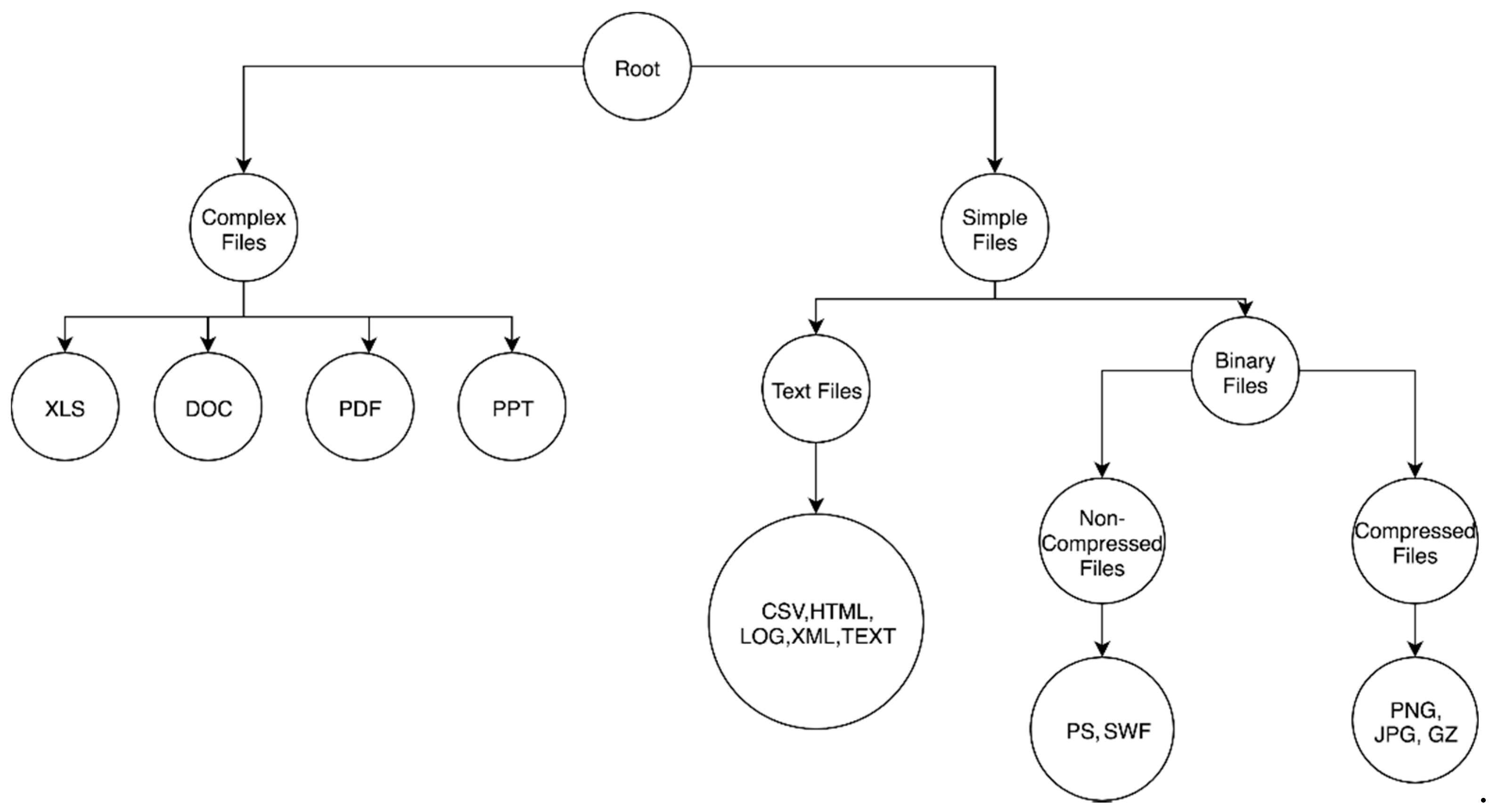
The first problem to tackle is the definition of the hierarchy. In our case, we have 14 different file types from which we extracted the fragments. We define a primitive hierarchy for the file types, as shown in
Figure 1. The main idea behind defining a hierarchy is the following. In the first level, the files are differentiated according to their complexity, i.e., complex files are grouped as the first child and the non-complex files are grouped as the second child. Complex files are the files that allow other simple files to be embedded in them, such as pdf and doc files. If the files are non-complex, then they are further classified into text files vs. binary files. This classification is valid, as the files are either text or binary. Moreover, the binary files can be further subclassified into compressed files and non-compressed files. If we have a new file that we need to assign to this hierarchy, we can follow the above-specified guidelines.
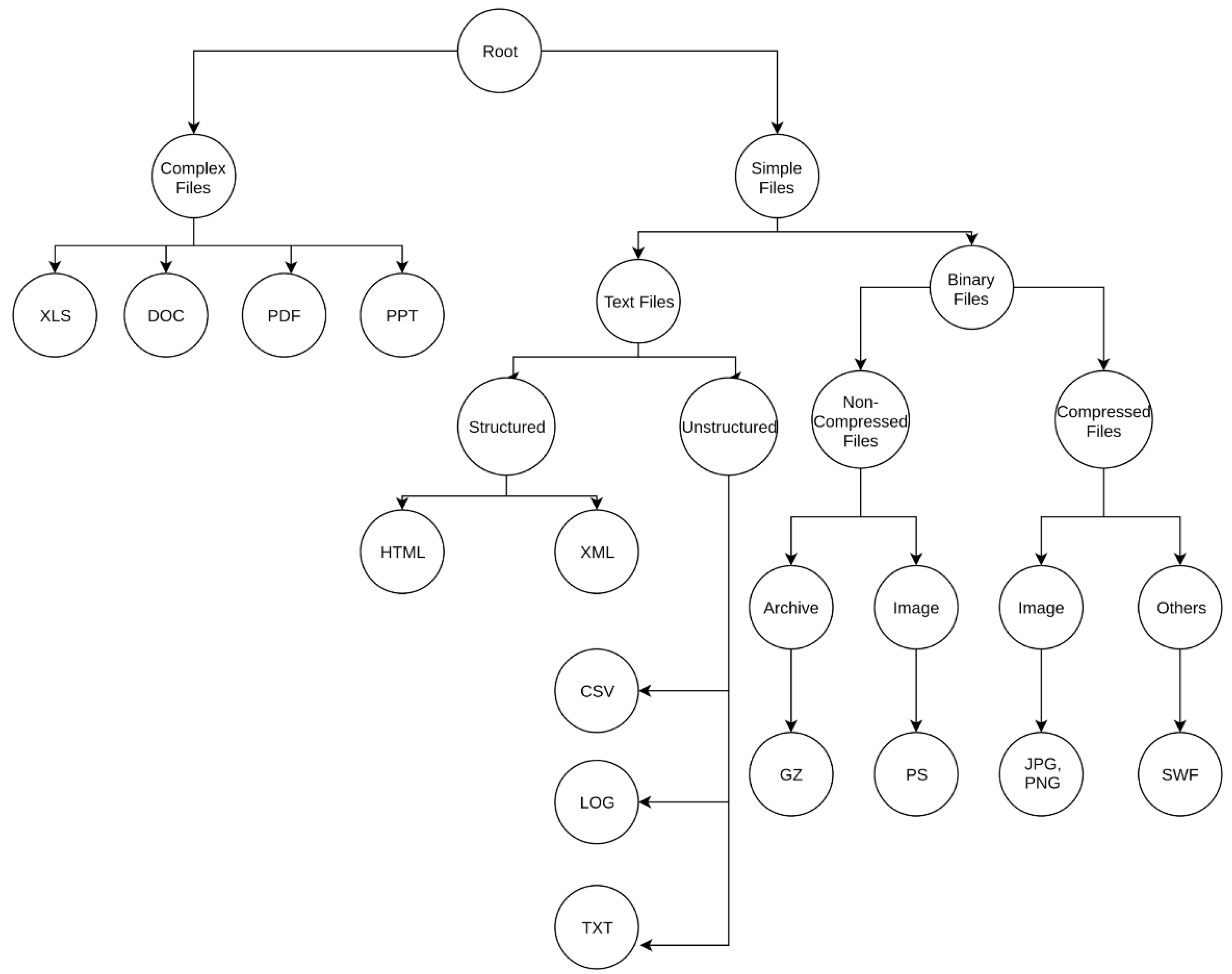
For the second hierarchy shown in
Figure 2, we differentiated the text file branch by considering if the file was structured or unstructured, i.e., if they contained tags (e.g., HTML/XML tags) that structured different parts of the files or not. Furthermore, binary files were specified as being high entropy files or low entropy files. High or low entropy files are the files that have high unigram entropy or low unigram entropy, respectively. Under high entropy files we differentiated between archives and images, while under low-entropy files we distinguished between images and other file-encoded formats.
A critical advantage of defining a hierarchical classification such as this is that if an investigator takes one file fragment and does one pass through the classifier, they can categorically understand the content of the file. For instance, if a gz (GNU Zip file type) fragment has been classified as a jpg fragment, and the path followed is root:binaryfiles:highentropy:image:jpg, the investigator can know that the file fragment is high entropy even, though the file fragment was misclassified at the final level. This enables the user of such a classifier to obtain partial information about the file fragment correctly, even if the final information might be incorrect.
Finally, encrypted files are beyond the scope of our present work because the features we used are not characteristic of encryption. However, the proposed technique could be used to identify encrypted file types after re-engineering features.
3.3. Feature Descriptions
We extracted a total of 10 features from each fragment, as shown in
Table 1. We used a feature ranking metric called information gain and found that these features were the most relevant, with metric values ranging from 0.229 ± 0.003 to 3.807 ± 0, and with the lowest being the Hamming weight and the highest being for the mean of the unigram counts. Hence, all the extracted features are relevant to the problem at hand.
3.4. Unigram Count Distribution
At the byte level, we only have 256 different values, regardless of the ASCII range. Unigram count distribution refers to the frequency of occurrence of these values in the file. Moreover, to decrease the number of dimensions and to escape the curse of dimensionality [
38], instead of using all 256 values in our feature, we fit this set to a normal distribution. As a normal distribution can be characterized completely by its mean and standard deviation, we use these two values per fragment as our features.
3.5. Entropy and Bigram Distribution
Similar to the Unigram Count Distribution, in this case, we find the frequency of occurrence of two-byte sequence (bigram) in the file, fit it to a normal distribution, and use the mean and standard deviation after fitting as our feature vectors. Furthermore, we also compute Shannon’s entropy [
26] for the bigram distribution and use it as another dimension in our feature space.
3.6. Contiguity
We computed the average contiguity between bytes (i.e., the average distance between consecutive bytes) for each file fragment.
3.7. Mean Byte Value
The mean byte value was one of the features included by Conti et al. [
6]. The mean byte value is simply the sum of the byte values in a given fragment divided by the fragment size.
3.8. Longest Streak
The largest number of continuous occurrences of the same byte in a file is known as its longest streak.
3.9. Compressed Length
We used the compression length as one of our features to approximate the Kolmogorov complexity of the file fragment [
27].
3.10. Hamming Weight
We calculated the Hamming weight of a file fragment by dividing the total number of ones by the total number of bits in the file fragment.
3.11. Evaluation Metrics
To evaluate our classifier on the dataset, we defined the following metrics. The i in the equations below refers to the instances.
3.12. Precision
Precision is defined as the ratio of the total number of true positives to the sum of the true positives and false positives, as in the following equation:
The recall is also known as the true positive rate and is defined as the ratio of the total number of true positives to the sum of the total number of true positives and false negatives.
3.13. F1-Measure
The F1-measure provides an average metric to the classification metrics of precision and recall. The F1-measure is defined as the harmonic mean between precision and recall. It can be represented mathematically as:
4. Experiment Details
We downloaded the zip files labeled
000.zip–073.zip from the Garfinkel corpus [
22]. Then, we dropped the first and last byte sets to ensure the headers and footers do not skew the results. We created 512-byte-sized fragments from each file type and created our dataset, which consisted of the file types and fragments, as shown in
Table 2. Then, we randomly sampled 1000 pieces of fragments from each file type to achieve a balanced dataset, as directly using the unbalanced dataset in a model can cause temporary or permanent bias. We extracted the features mentioned in the previous section from the file fragments. Finally, we defined our hierarchy, as shown in
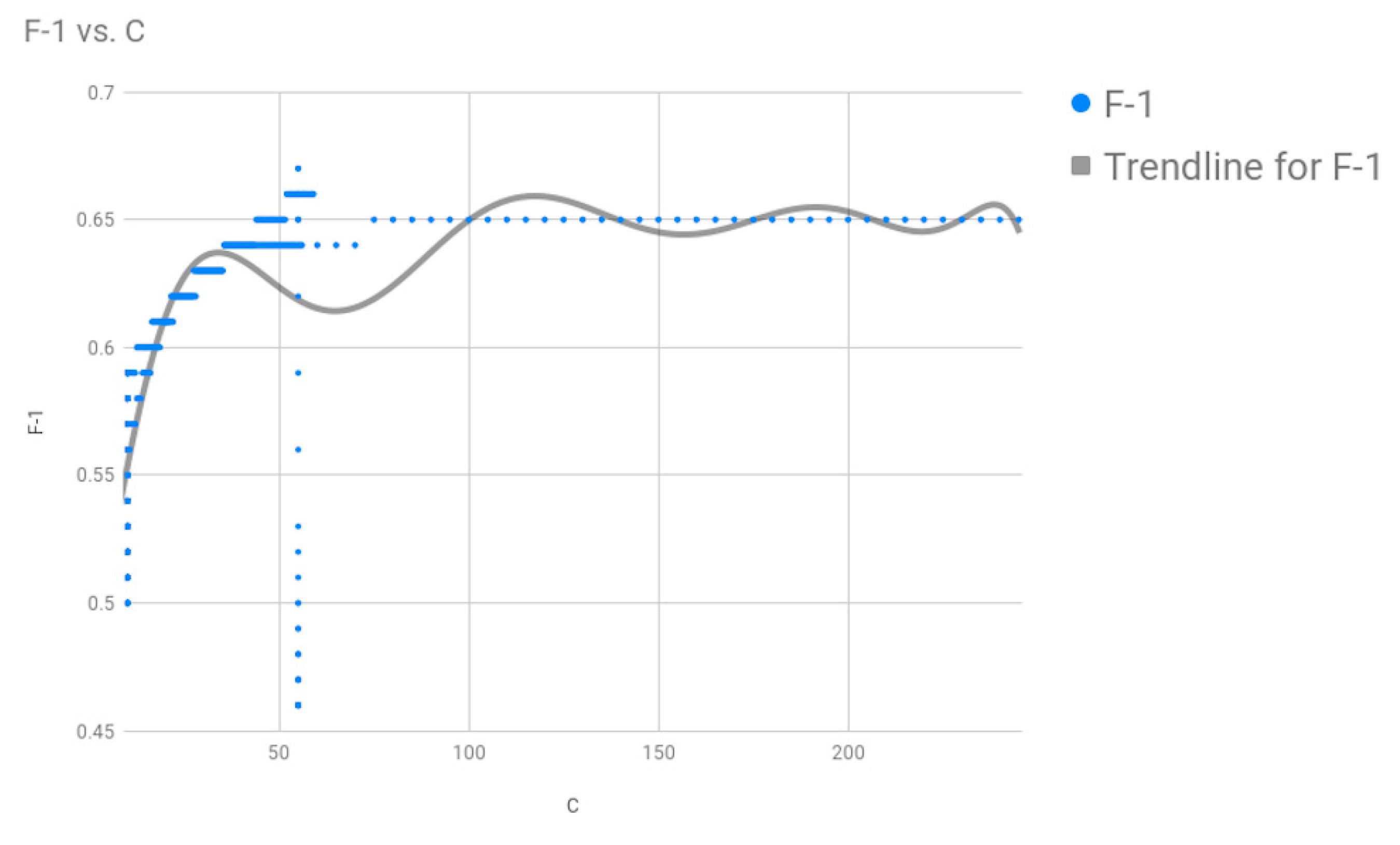
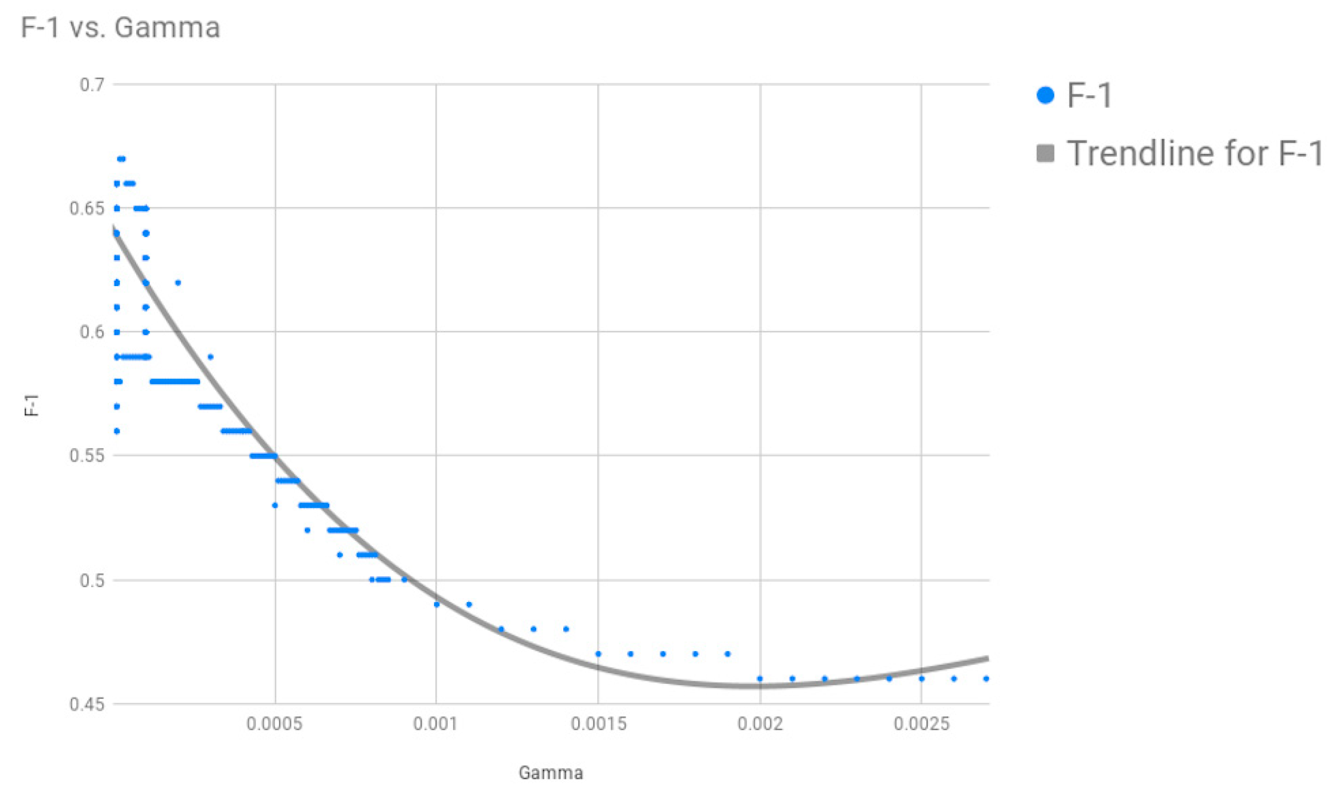
Figure 1, and performed 10-fold cross-validation on our model with the dataset. Upon optimizing the SVM parameters using grid search, we found that we got the best results for the two parameters of the Radial Basis Function (RBF) Kernel: cost
C = 75, gamma = 0.0001, where our search space for C was [0, 100] and for gamma was [0.0001, 2].
After conducting the experiment on a primitive hierarchy, as shown in
Figure 1, we decided to further extend our hierarchy on the binary branch and came up with another hierarchy (
Figure 2). We tested our hierarchical classifier against the dataset using our modified hierarchy and obtained a second set of results.
We performed our experiments on the server made of 48 processors and 256 GB of RAM. We implement our proposed hierarchical classification algorithm in Python (Scikit-learn libraries) and ran the experiments on a Linux operating system.
Table 3 shows the time requires for each step of the experiments. The most time-consuming part is the grid search, which is used to find the best parameter (C and Gamma) for the support vector machine (SVM) algorithm. This process takes around 8.5 days to complete. After selecting the best parameter, we trained and tested the dataset using 10-fold cross-validation, which takes only 183.12 s to complete. To improve the performance of our algorithm, we ran 10-fold cross-validation in parallel using all 48 processors in the server.
As our dataset is not that large, we did not compare our method with a deep learning algorithm. Deep learning requires high computational resources [
31] and a large amount of data to perform well. The computational complexity of the deep learning method depends not only on the dataset size but also on the network architecture. A deep learning network may consist of many hidden layers and nodes, which makes it computationally expensive to train. Often the models are trained using graphics processing units (GPUs) rather than CPUs to overcome this problem. It is possible to achieve better performance using non-deep-learning methods with much less computational resources and less data [
39].
6. Comparison with Previous Works and Discussion
The recall rate of our classifier is significantly higher than a random choice (1/14~0.071). Our accuracy, defined as the ratio of the sum of TP (True Positive) and TN (True Negative) over the sum of TP, TN, FP (False Positive), and FN (False Negative), for various folds for the first experiment, is shown in
Table 6.
Our classifier outperformed other directly comparable classifiers in previous works, as shown in
Table 7. In particular, Fitzgerald et al. [
15] obtained an average prediction accuracy of 49.1%. Moreover, Axelsson [
5] was able to achieve a prediction accuracy of 34% for 28 file types. Additionally, Veenman was able to achieve a prediction accuracy of 45% for 11 file types. Xu [
16] used 29 file types and obtained an average accuracy of 54.7%. For the fourteen file types in our study, the accuracy for each file type is shown in
Table 7. On average, for the 14 file types which we used, the average accuracy of detection was highest for Fitzgerald at 57.51%. These researchers used the same Digital Corpora, known as govdocs1 corpus, with random sampling.
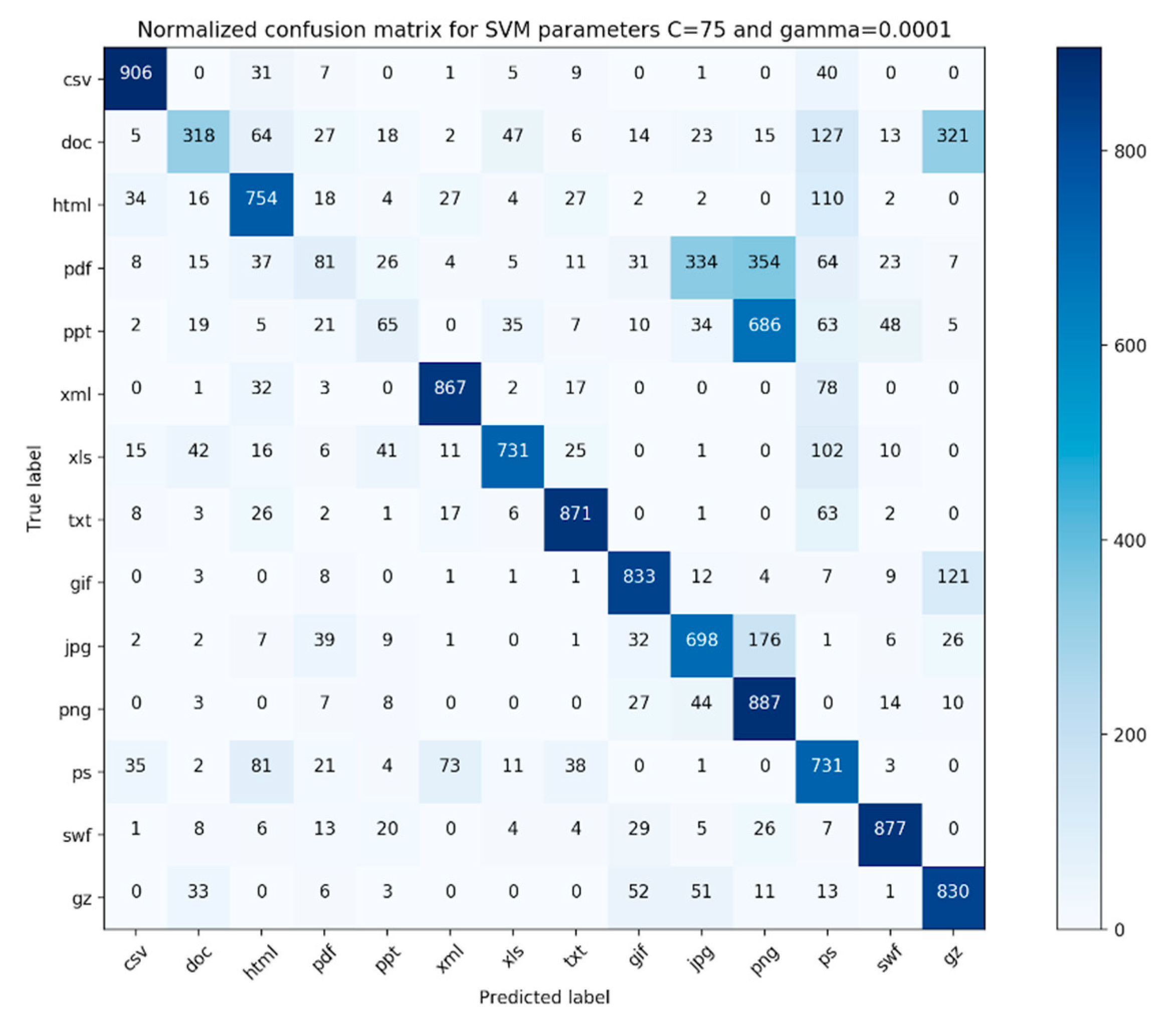
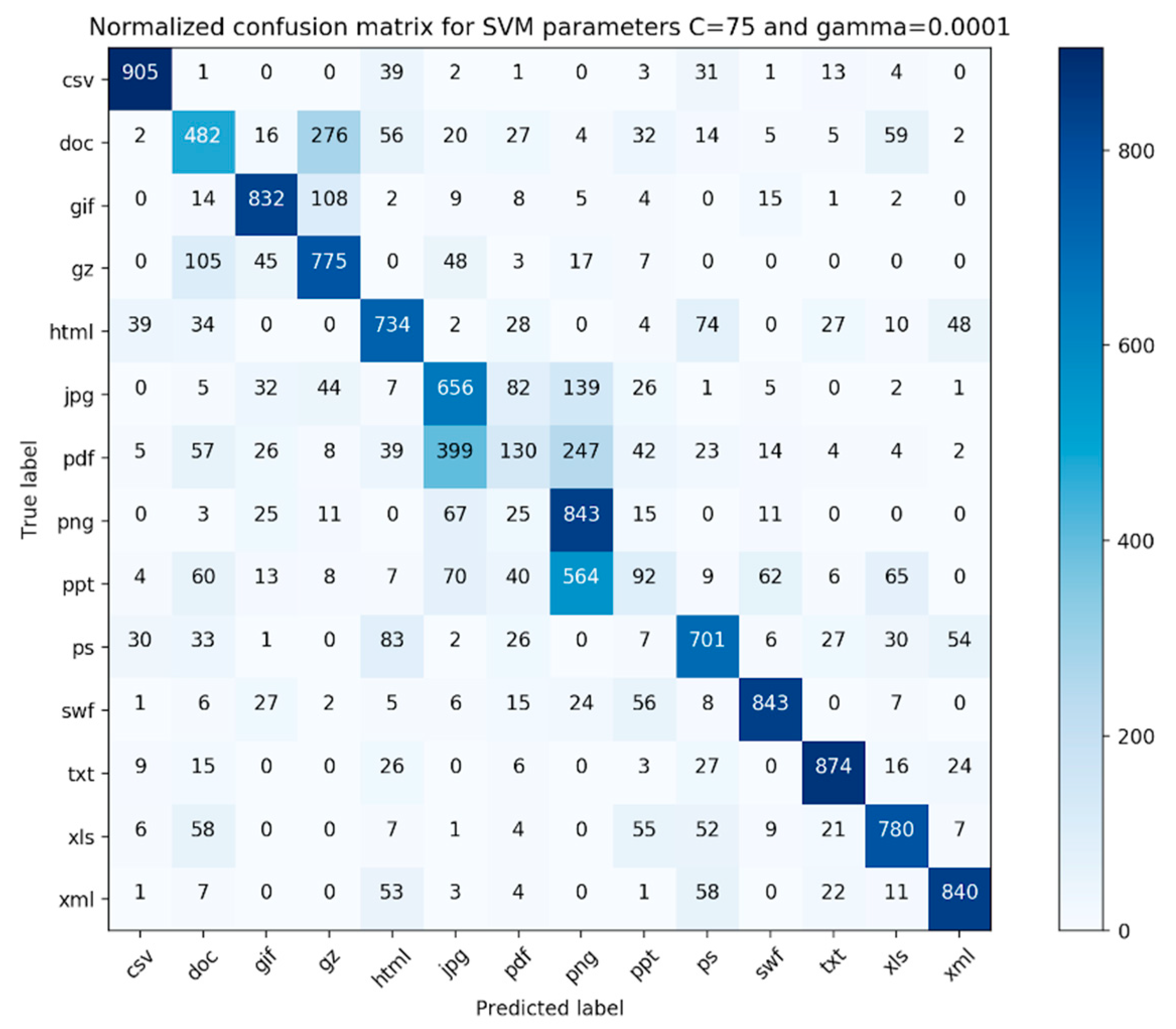
The confusion matrix for our evaluation experiments is shown in
Figure 5 and
Figure 6. Each file type had 1000 fragments in the data. As we can see from the confusion matrix, the classifier performs well on files that are simple file fragments (e.g., plain text files, png files) and worse on complex files (e.g., pdf, ppt, and doc). Additionally, from
Table 3 and
Table 4, we found that the
TPR (True Positive Rate) rates for these file types were lower compared to other file types.
For simple files, our proposed method achieves better results for xml (
Table 4) files compared to html files in terms of F1-measure values. The F1-measure values of xml and html files are 0.85 vs. 0.71, respectively. This is because xml defines data separately from their presentation, which makes xml data easier to locate and manipulate. The xml file mainly focuses on the transfer of data, while html focuses on the presentation of the data. The higher heterogeneity of contents that usually exist in html files also makes it difficult to classify html files. For other simple files, namely jpg and png, the classifier achieves average F1-measure values of 0.57 and 0.59, respectively. This result is due to the fact both jpg and png use compression methods (DCT (Discrete Cosine Transform) and LZW (Lempel-Ziv-Welch)) to minimize the size of the image.
Upon examination of the pdf files, we found that the file fragments belonging to the pdfs that were misclassified consisted of a large portion of images.
Table 8 shows the percentage of complex files that contain the image in our dataset. About 90.76% of ppt files and 58.30% of pdf files contain image, while the F1-measures for ppt and pdf files are 0.14 and 0.19, respectively. For doc files, only 3.07% of files contained image and the F1-measure for the doc file is 0.51. Therefore, it is evident that images in complex files have a significant impact on the file fragment classification.
Moreover, the pdf files usually store an image as a separate object that contains the raw binary data of the image. Images are not embedded inside a pdf as tif, gif, bmp, jpeg, or png formats. The image bytes are modified when the pdf is created and different pdf creation tools may store the same image in very different ways. After analyzing the metadata of pdf files in our dataset, we found that the pdfs are created by 573 different pdf creator software programs (including different versions). Moreover, the pdf creator software produce different versions of pdf files. This suggests that our hierarchy needs fine-tuning with regards to complex files, as currently all complex files are placed under the same parent node.
7. Conclusions and Future Works
File fragment classification is of paramount importance in digital forensics. In this work, we explored a classification approach called hierarchical classification for file fragment classification. Owing to its hierarchical nature, if a correct taxonomy is found we believe that this could be a general technique used for fragment classification. Here, we used support vector machines (SVMs) as our base classifiers and also proposed a hierarchical taxonomy for files, such that if a new file is introduced and this technique needs to be used then this is made possible. Furthermore, we investigated the effects of the hyperparameters C and gamma and found that the parameters best suited to our model had values of C = 75 and gamma = 0.0001. Then, we also tested our classification technique using a dataset consisting of 14 file types and with 1000 fragments, each having 512-byte fragments for each file type, via 10-fold cross-validation technique. Furthermore, we refined our first hierarchy slightly and conducted the same experiment on the same dataset. We compared the F1 measures for both our experiment runs to see if refining our hierarchy would help in the classification process.
Our classifier either outperformed or gave comparable results to all preceding similar classifiers suggested in the literature. From the confusion matrix presented in
Figure 5 and
Figure 6, we discovered that our classifier worked best for simple file types and worst for complex file types. On further examination, it was found that some of the file fragments in the pdf category that were incorrectly classified consisted of a lot of pictures. We believe that the features utilized in this study are not adequate, as none of our features characterize the membership relationship between the file fragment and its parent class, especially for complex file types. Moreover, after refining the simple file branch in terms of the hierarchical complexity, we found that our classifier performed better for complex file types. This suggests that we need to further fine-tune our hierarchy branch for complex files or completely eliminate it and make our hierarchy completely file-content-based. Furthermore, it was interesting that most of the incorrectly classified file fragments belonging to the jpg file type were classified as png file fragments. This suggests that a deeper look needs to be taken towards engineering other features that can characterize the membership relationship of a file fragment with its parent file type.
The results of the hierarchical classification approach to file fragment classification problems are quite promising, and we believe that our approach has provided a different perspective (i.e., a hierarchical perspective) for looking at and solving this complex problem. Here, we can see several areas of research in the future. Firstly, we believe that a fuzzy metric should be developed and a membership function should be defined to characterize the membership of complex and simple file categories. This would eliminate the need for having a complex file type branch, and these files could be represented merely by the superposition of simple file types. Secondly, the hierarchy we proposed needs to be further tuned, such that the misclassifications can be eliminated. Additionally, encrypted files need to be introduced into the hierarchy somehow. Research should be directed toward finding a way to include standard pattern-matching-based fragment classification and the hierarchical classification technique. Pattern matching could be included as a feature in the classification process. Thirdly, the effects of different pdf creation tools and pdf versions should be further analyzed. Additionally, the govdocs1 corpus does not contain zip files or recent Microsoft Office formats (i.e., docx, xlsx, pptx). These new file formats also need to be analyzed. Moreover, new Microsoft Office formats (docx, xlsx, pptx) use file archiving computer program, named PKZIP (written by Phil Katz), to compress content, so it will be interesting to see the comparison of both old and recent Microsoft Office formats with other compressed file formats (i.e., gz and zip). Another interesting research topic could be the analysis of the effects of the defragmentation tool. Usually, files are stored in different sectors in a disk as fragments, which are not contiguous. Defragmentation tools are used to move these file fragments to make them contiguous. Finally, the use of other classification techniques as base classifiers needs to be investigated, such that researchers can choose the classifier that best suits their needs and interests.


 and
and 


