Semi-Supervised Adversarial Variational Autoencoder


Cedric-Lab, CNAM, HESAM Université, 292 rue Saint Martin, CEDEX 03, 750141 Paris, France
Mach. Learn. Knowl. Extr. 2020, 2(3), 361-378; https://0-doi-org.brum.beds.ac.uk/10.3390/make2030020
Submission received: 1 August 2020
/
Revised: 1 September 2020
/
Accepted: 3 September 2020
/
Published: 6 September 2020
Abstract
:We present a method to improve the reconstruction and generation performance of a variational autoencoder (VAE) by injecting an adversarial learning. Instead of comparing the reconstructed with the original data to calculate the reconstruction loss, we use a consistency principle for deep features. The main contributions are threefold. Firstly, our approach perfectly combines the two models, i.e., GAN and VAE, and thus improves the generation and reconstruction performance of the VAE. Secondly, the VAE training is done in two steps, which allows to dissociate the constraints used for the construction of the latent space on the one hand, and those used for the training of the decoder. By using this two-step learning process, our method can be more widely used in applications other than image processing. While training the encoder, the label information is integrated to better structure the latent space in a supervised way. The third contribution is to use the trained encoder for the consistency principle for deep features extracted from the hidden layers. We present experimental results to show that our method gives better performance than the original VAE. The results demonstrate that the adversarial constraints allow the decoder to generate images that are more authentic and realistic than the conventional VAE.
1. Introduction
Deep generative models (DGMs) are part of the deep models family and are a powerful way to learn any distribution of observed data through unsupervised learning. The DGMs are composed mainly by variational autoencoders (VAEs) [1,2,3,4], and generative adversarial networks (GANs) [5]. The VAEs are mainly used to extract features from the input vector in an unsupervised way while the GANs are used to generate synthetic samples through an adversarial learning by achieving an equilibrium between a Generator and a Discriminator. The strength of VAE comes from an extra layer used for sampling the latent vector z and an additional term in the loss function that makes the generation of a more continuous latent space than standard autoencoders.
The VAEs have met with great success in recent years in several applicative areas including anomaly detection [6,7,8,9], text classification [10], sentence generation [11], speech synthesis and recognition [12,13,14], spatio-temporal solar irradiance forecasting [15] and in geoscience for data assimilation [2]. In other respects, the two major application areas of the VAEs are the biomedical and healthcare recommendation [16,17,18,19], and industrial applications for nonlinear processes monitoring [1,3,4,20,21,22,23,24,25].
VAEs are very efficient for reconstructing input data through a continuous and an optimized latent space. Indeed, one of the terms of the VAE loss function is the reconstruction term, which is suitable for reconstructing the input data, but with less realism than GANs. For example, an image reconstructed by a VAE is generally blurred and less realistic than the original one. However, the VAEs are completely inefficient for generating new synthetic data from the latent space comparing to the GANs. Upon an adversarial learning of the GANs, a discriminator is employed to evaluate the probability that a sample created by the generator is real or false. Most of the applications of GANs are focused in the field of image processing such as biomedical images [26,27], but recently some papers in the industrial field have been published, mainly focused on data generation to solve the problem of the imbalanced training data [28,29,30,31,32,33]. Through continuous improvement of GAN, its performance has been increasingly enhanced and several variants have recently been developed [34,35,36,37,38,39,40,41,42,43,44,45,46,47,48,49,50,51].
The weakness of GANs lies in their latent space, which is not structured similarly to VAEs due to the lack of an encoder, which can further support the inverse mapping. With an additional encoding function, GANs can explore and use a structured latent space to discover “concept vectors” that represent high-level attributes [26]. To this purpose, some research has been recently developed, such as [48,52,53,54,55].
In this paper, we propose a method to inject an adversarial learning into a VAE to improve its reconstruction and generation performance. Instead of comparing the reconstructed data with the original data to calculate the reconstruction loss, we use a consistency principle for deep features such as style reconstruction loss (Gatys [56]). To do this, the training process of the VAE is divided into two steps: training the encoder and then training the decoder. While training the encoder, we integrate the label information to structure the latent space in a supervised way, in a manner similar to [53,55]. For the consistency principle for deep features, contrary to [56] and Hou [54] who used the pretrained deep convolutional neural network VGGNet [57], we use the features extracted from the hidden layers of the encoder. Thus, our method can be applied to areas other than image processing such as industrial nonlinear monitoring or biomedical applications. We present experimental results to show that our method gives better performance than the original VAE. In brief, our main contributions are threefold.
- Our approach perfectly combines the two models, i.e., GAN and VAE, and thus improves the generation and reconstruction performance of the VAE.
- The VAE training is done in two steps, which allows to dissociate the constraints used for the construction of the latent space on the one hand, and those used for the training of the decoder.
- The encoder is used for the consistency principle for deep features extracted from the hidden layers.
The rest of the paper is organized as follows. We first briefly review the generative models in Section 2. After that, in Section 3, we describe the proposed method. Then, in Section 4, we present experimental results, which show that the proposed method improves the performance of VAE. The last section of the paper summarizes the conclusions.
2. Generative Networks and Adversarial Learning
2.1. Autoencoder and the Variational Form
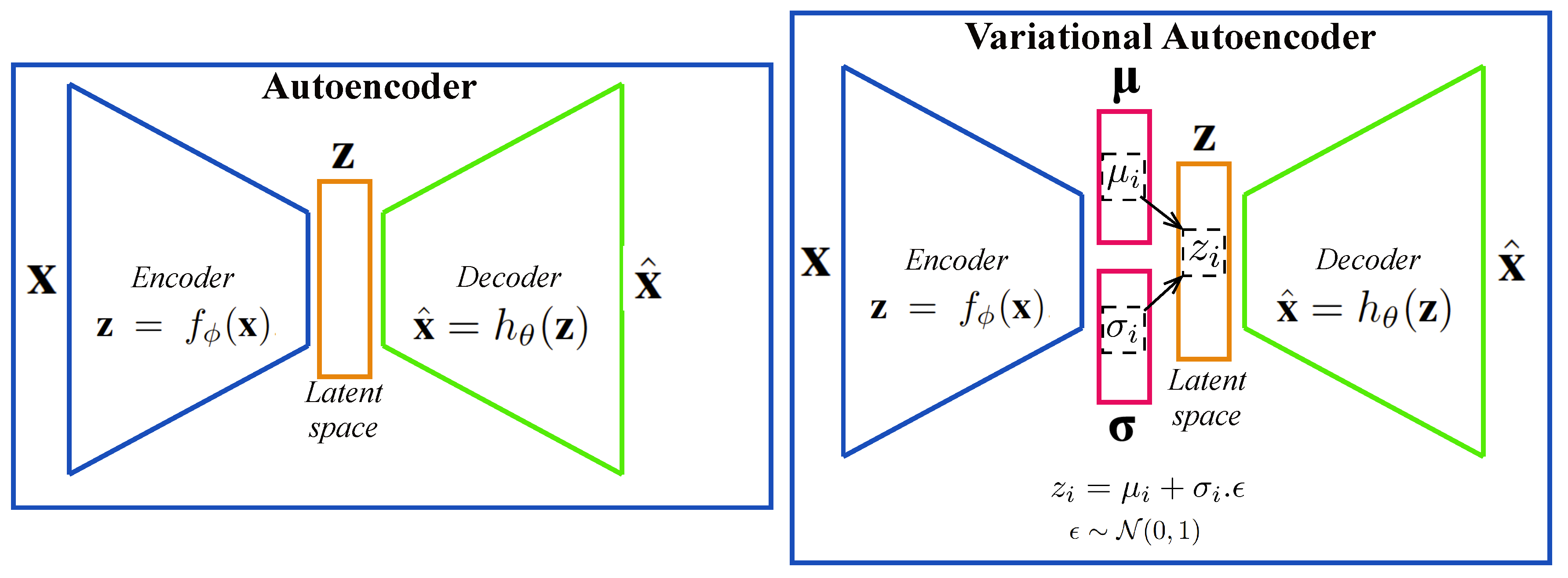
Autoencoder (AE) represents one of the first generative models trained to recreate or reproduce the input vector [58,59,60,61]. The AE is composed by two main structures: an encoder and a decoder (Figure 1), which are multilayered neural networks (NNs) parameterized by and , respectively. The first part encodes the input data into a latent representation by the encoder function , whereas the second NN decodes this latent representation onto which is an approximation or a reconstruction of the original data. In an AE, an equal number of units are used in the input/output layers while fewer units are used in the latent space (Figure 1).
The variational form of the AE (Figure 1) becomes a popular generative model by combining the Bayesian inference and the efficiency of the NNs to obtain a nonlinear low-dimensional latent space [1,2,3,4]. The Bayesian inference is obtained by an additional layer used for sampling the latent vector with a prior specified distribution , usually assumed to be a standard Gaussian , where is the identity matrix. Each element of the latent layer is obtained as follows:
where and are the components of the mean and standard deviation vectors, is a random variable following a standard Normal distribution (). Unlike the AE, which generates the latent vector , the VAE generates vector of means and standard deviations . This allows to have more continuity in the latent space than the original AE. The VAE loss function given by Equation (2) has two terms. The first term is the reconstruction loss function (Equation (3)), which allows to minimize the difference between the input and output instances.
Both the negative expected log-likelihood (e.g., the cross-entropy function) and the mean squared error (MSE) can be used. When the sigmoid function is used in the output layer, the derivatives of MSE and cross-entropy can have similar forms.
The second term (Equation (4)) corresponds to the Kullback–Liebler () divergence loss term that forces the generation of a latent vector with the specified Normal distribution [62,63]. The divergence is a theoretical measure of proximity between two densities and . It is asymmetric () and nonnegative. It is minimized when [64]. Thus, the divergence term measures how close the conditional distribution density of the encoded latent vectors is from the desired Normal distribution . The value of is zero when two probability distributions are the same, which forces the encoder of VAE to learn the latent variables that follow a multivariate normal distribution over a k-dimensional latent space.
2.2. Adversarial Learning
One of the major advantages of the Variational form compared to the classic version of the AE is achieved using the Kullback–Liebler divergence loss term (), which ensures that the encoder will organize the latent space with good properties for the generative process. Instead of encoding an input as a single point, a Normal distribution is associated with encoding each input instance. This continuity of latent space allows the decoder not only to be able to reproduce an input vector, but also to generate new data from the latent space. However, the reconstruction loss function is not effective for data generation compared to the adversarial learning technics [5]. The main idea of these methods is to create an additional NN, called a discriminator , that will learn to distinguish between the real data and the data generated by the generator .
The learning process then consists in successively training the generator to generate new data and the discriminator to dissociate between real and generated data (Figure 2). The learning process converges when the generator reaches the point of luring the discriminator. The discriminator is optimized by maximizing the probability of distinguishing between real and generated data while the generator is trained simultaneously to minimize . Thus, the goal of the whole adversarial training can be summarized as a two-player min-max game with the value function [5]:
where and . These techniques are much more efficient than the reconstruction loss function for generating data from a data space, for example, the latent space of VAE. Unlike the latent space of the VAE where the data are structured according to the Kullback–Liebler divergence loss term that forces the generation of a latent vector with the specified Normal distribution, the data space of the GAN is structured in a random way, making it less efficient in managing the data to be generated.
3. Proposed Method
3.1. Method Overview
The method proposed in this paper, which is presented in Figure 3, consists of separating the learning of the VAE into two successive parts: the learning of the encoder followed by the learning of the decoder . This decoupling between encoder and decoder during the learning phase allows a better structuration of the latent encoder space to focus in a second step on the optimization of the decoder.
In order to structure the latent space taking into account the label information, a classifier is trained at the same time as the encoder . Two optimization functions are then used during the first phase: the Kullback–Liebler divergence loss function and the categorical cross-entropy .
At the convergence of the first phase, the two models thus obtained, i.e., the encoder and the classifier , will be used to train the decoder . Three optimization functions are then used for this second step:
- A reconstruction loss function ()
- An adversarial loss function ()
- A latent space loss function ()
As previously used by Hou [54], instead of comparing the reconstructed data with the original one to calculate the reconstruction loss, we compare some features extracted from the encoder as a style reconstruction loss (Gatys [56]). A feature reconstruction loss function is then used instead of a data reconstruction loss function. To calculate these features, we use the encoder thus obtained by the first learning phase instead of using a pretrained deep convolutional neural network such as the VGGNet network [57] used by Gatys [56] and Hou [54].
In order to facilitate the convergence of the decoder, two further optimization terms are included in the whole loss function: an adversarial loss function obtained with the help of a discriminator , trained at the same time as the decoder , and a latent space loss function . This supplementary term will compare the original latent space with the reconstructed one thanks to the classifier obtained during the first learning phase.
3.2. First Step: Training the Variational Encoder Classifier
In this first step, the encoder and classifier are stacked together in order to form the Variational Encoder Classifier (VEC). The whole structure is trained at the same time using the following loss function :
where corresponds to the Kullback–Liebler () divergence loss term given by Equation (4), while the second term represents the categorical cross-entropy obtained by the following expression:
where y is the target label and is the statistical expectation operator. Algorithm 1 presents the complete procedural steps of this first learning phase.
| Algorithm 1 Training the VEC Model |
 |
3.3. Second Step: Training the Decoder
The encoder as well as the classifier obtained from the previous phase will therefore be frozen and used to train the decoder. The global optimization function is given by the following expression where and are fitting parameters:
The first term allows the decoder to enhance its input reconstruction properties, while the second term allows it to increase its ability to generate artificial data from latent space. These two terms will be put in competition and it will be necessary to find the best compromise thanks to the fitting parameters. A third term will ensure that the virtual data generation is done respecting the distribution of classes in the latent space. The whole training process of the decoder is presented by Algorithm 2.
| Algorithm 2 Training the Decoder Model |
 |
3.3.1. Feature Reconstruction Loss
For the reconstruction optimization function, we adopt the method proposed by Gatys [56], which consists of extracting the style of an image from the first hidden layers of a pre-trained network. It is also the same principle used by Lin [65] as Feature Pyramid Networks for Object Detection. Thus, instead of calculating the reconstruction error between the input and the output of the decoder, the reconstruction error is calculated from the features of the image. As an alternative to a generic pre-trained network, such as the VGGNet network [57] used by [56] and Hou [54], we will exploit the features extracted from the previously trained encoder. The advantage of our method is to adapt the extracted features to the type of application being studied, which may be outside the scope of the images learned by the VGGNet network. Thus, our approach can be applied to biomedical images such as histopathological images [27,66] or vibration signals from a mechatronic system for industrial monitoring [20].
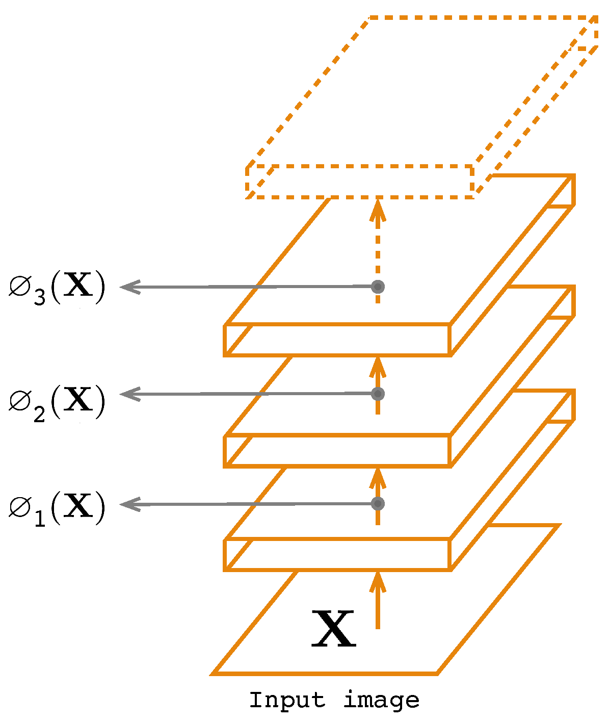
As shown in Figure 4, the first three layers of the encoder will be used to extract features from the input image . The characteristics of will then be compared to the characteristics of the output generated by the decoder. The optimization function is then given by the following expression:
where and are respectevely the features of and extracted from the layer i and is a fitting parameter.
3.3.2. Adversarial Loss
In addition to the reconstruction function, a second term allows the decoder to reconstitute the input data more realistically. A discriminator trained with the adversarial learning techniques presented in the previous section will feed a cost function that will penalize the decoder if the reconstructed image is not authentic. As in the works of [47], the output of the discriminator is linear with +1 label for real images and -1 for artificial images. However, to enhance the data generation effect, larger output values are possible, such as the ±10 output used by [54]. For this purpose, we prefer to adjust this generation effect with a fitting variable (Equation (8)). The update of the discriminator is done before each decoder training cycle. In order to increase this adversarial learning, we use the Wasserstein GAN method [47], which consists of increasing the number of learning cycles of the discriminator with respect to the generator. Algorithm 2 presents the detail of the discriminator training where the variable defines the number of training cycles of the discriminator.
The optimization function is then given by the following expression:
3.3.3. Latent Loss
A last term prevents the generation effect from being stronger than the reconstitution effect. The classifier obtained in the previous learning phase will make sure that the latent space obtained by the generated data has the same distribution as the original latent space Z. The label information of the input data is thus integrated in the reconstitution/generation process. The output of the classifier will penalize the decoder if the generated data does not belong to the same class as the original data. The expression of is defined by:
4. Experiments
4.1. Dataset Description
We experimented with our method on four databases: The MNIST [67], The Omniglot dataset [68], The Caltech 101 Silhouettes dataset [69] and Fashion-MNIST [70], which are briefly described below. Figure 5 illustrates some of the images taken randomly from the four databases.
- The MNIST [67] is a standard database that contains images of ten handwritten digits (0 to 9) and is split into 60,000 samples for training and 10,000 for the test.
- The Omniglot dataset [68] contains images of handwritten characters from many world alphabets representing 50 classes, which is split into 24,345 training and 8070 test images.
- The Caltech 101 Silhouettes dataset [69] is composed of images representing object silhouettes of 101 classes and is split into 6364 samples for training and 2307 for the test.
- Fashion-MNIST [70] contains images of fashion products from 10 categories and is split in 60,000 samples for training and 10,000 for the test.
4.2. Neural Network Architecture
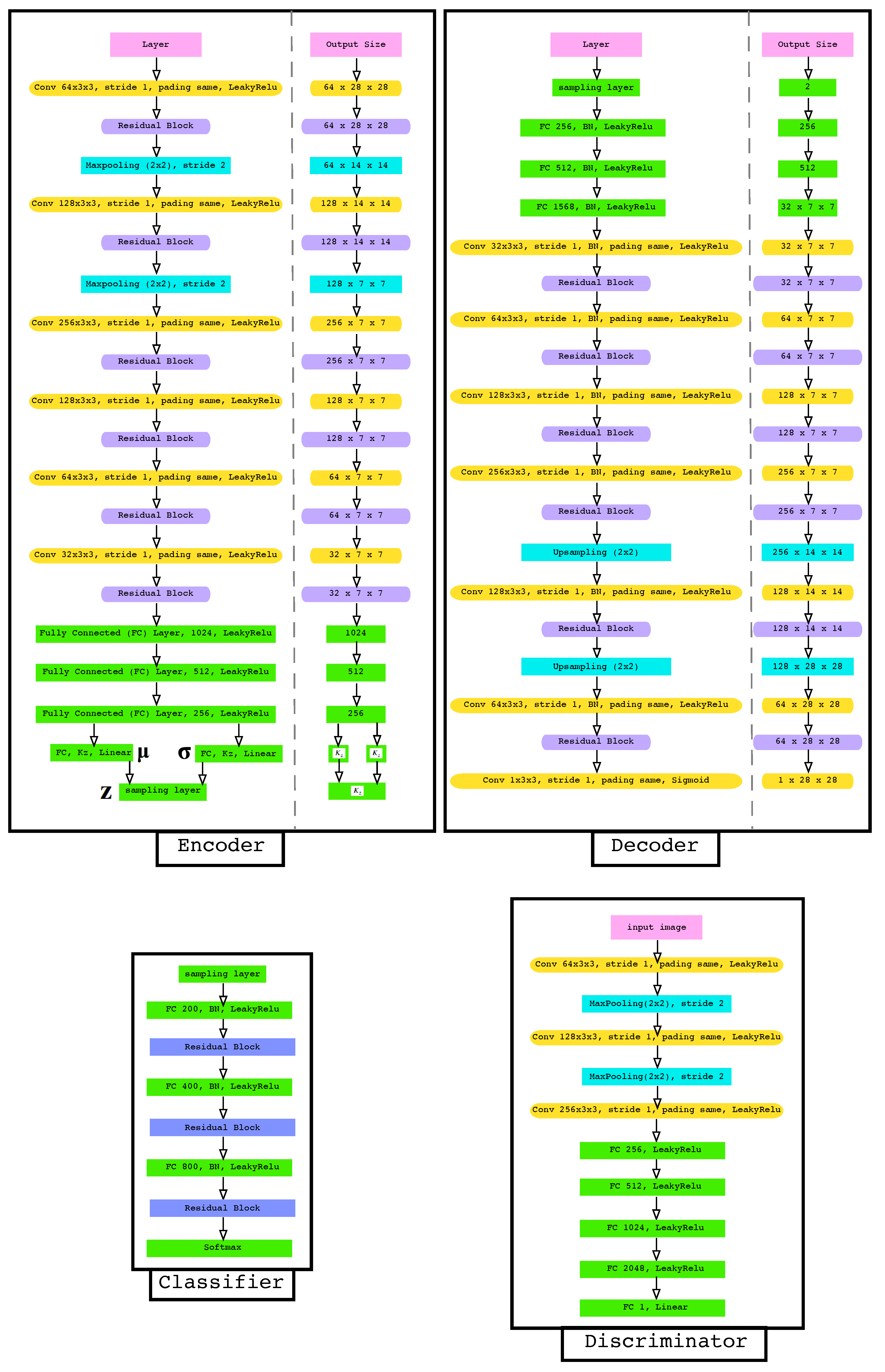
As shown in Figure 6, both the encoder and decoder are deep residual convolutional neural networks. The encoder is composed of 6 convolutional layers with kernel and stride. To achieve spatial downsampling we used 2 maxpooling layers with kernel and stride. Each convolutional layer is followed by a residual block and a LeakyReLU activation layer. We used the same residual block as used by [54]. At the end of the encoder, three fully connected layers with a LeakyReLU activation are followed by two linear fully connected layers for mean and variance. The output of the encoder is given by the sampling layer.
For the decoder, we almost used the inverse encoder structure. The input of the decoder is the sampling layer followed by three fully connected layers with batch normalization and a LeakyReLU activation. Seven convolutional layers with kernel and stride followed by batch normalization, a LeakyReLU activation and residual block and 2 upsampling layers.
For the discriminator, we used 3 convolutional layers with kernel and stride LeakyReLU activation, 2 maxpooling layers with kernel and stride and 4 fully connected layers with a LeakyReLU activation. Lastly, the output of the discriminator was formed by one linear unit.
The classifier was formed by 3 fully connected layers with batch normalization and a LeakyReLU activation. Each fully connected layer is followed by a residual block. The output of the classifier was obtained by a softmax layer.
4.3. Experimental Focus
4.3.1. Impact of the Dimension Size of the Latent Space
It is obvious that the dimension of the latent space plays an active influence on the quality of reconstruction and data generation. The quality of VAE decoding is highly dependent on the size of the latent space. We then compared two configurations: a two-dimensional latent space () with a () dimensional space.
4.3.2. Impact of Weighting Parameters and
We also investigated the impact of the and weighting parameters of Equation (8). We set the parameters of the feature reconstruction loss (Equation (3)) to 1, 0.1 and 0.01 for i = 1, 2 and 3, respectively. To judge the influence of each parameter of adversarial loss and latent loss , we have varied the parameter in an increasing way according to two configurations of : and .
4.4. Results and Discussion
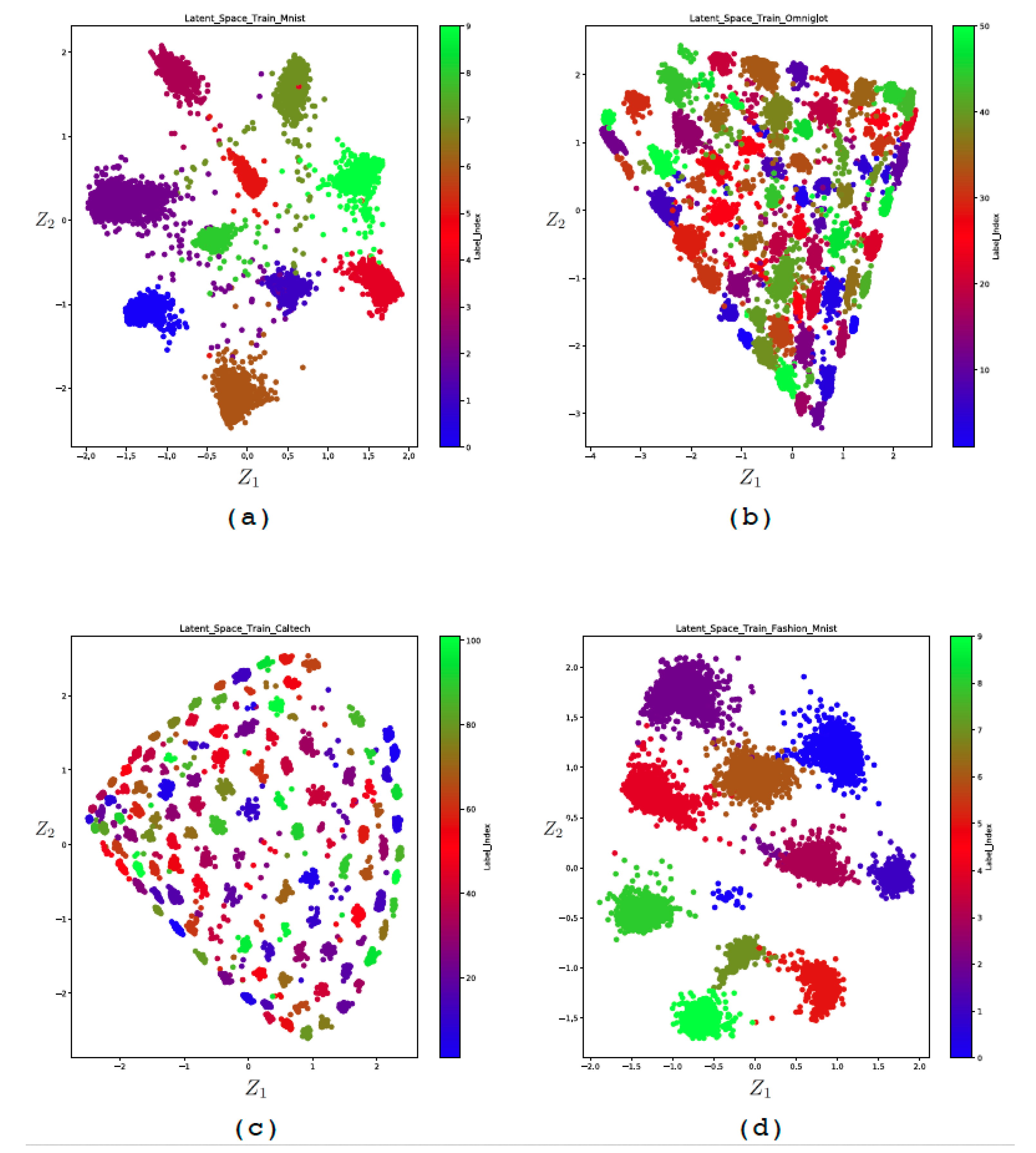
4.4.1. Supervised 2D-Latent Space
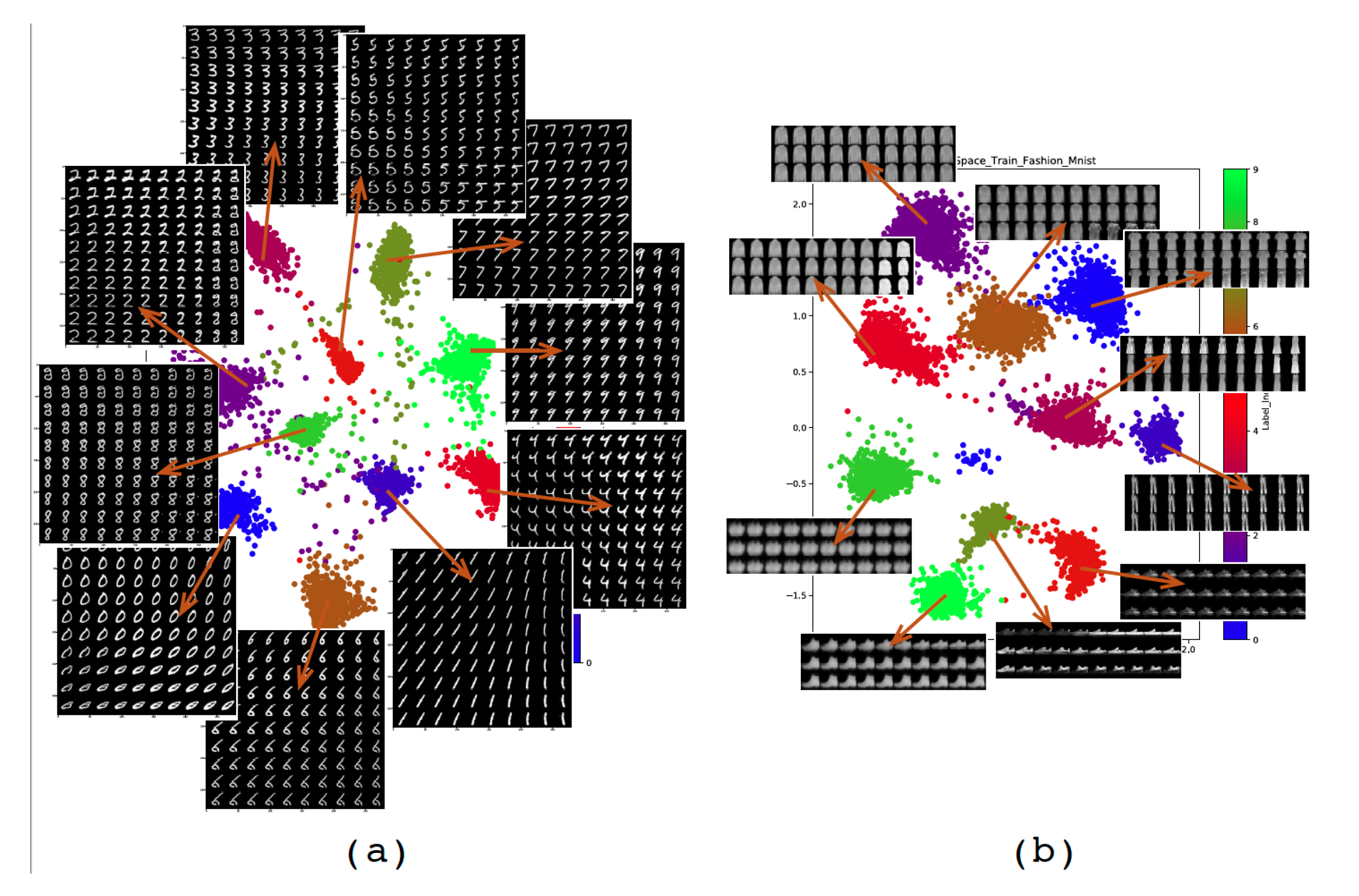
In order to visually analyze the latent space obtained by the encoder-classifier, we set the dimension of this space to 2 (). The interest of such a space is to be able to make a projection of the initial input data space to a space visually accessible to the human brain. We can thus visually analyze the quality of the encoder. Figure 7 shows the 2D latent space obtained for the four databases. We can then see the distribution of data in the latent space as well as the interaction between the different classes. We can thus analyze the overlaps between the classes. One can then choose the area of this latent space in order to generate artificial data. Figure 8 shows examples of images generated from the latent space for Mnist and Fashion Mnist, respectively. It is interesting to note that even in a space of reduced size, the data are organized according to a logic of likelihood between classes. This is very well illustrated by the latent space of Fashion Mnist where we can see that the three classes #5, 7, and 9, which represent the shoes, are grouped together. The handbag cluster is also isolated from the rest of the clusters.
4.4.2. Image Reconstruction and Generation
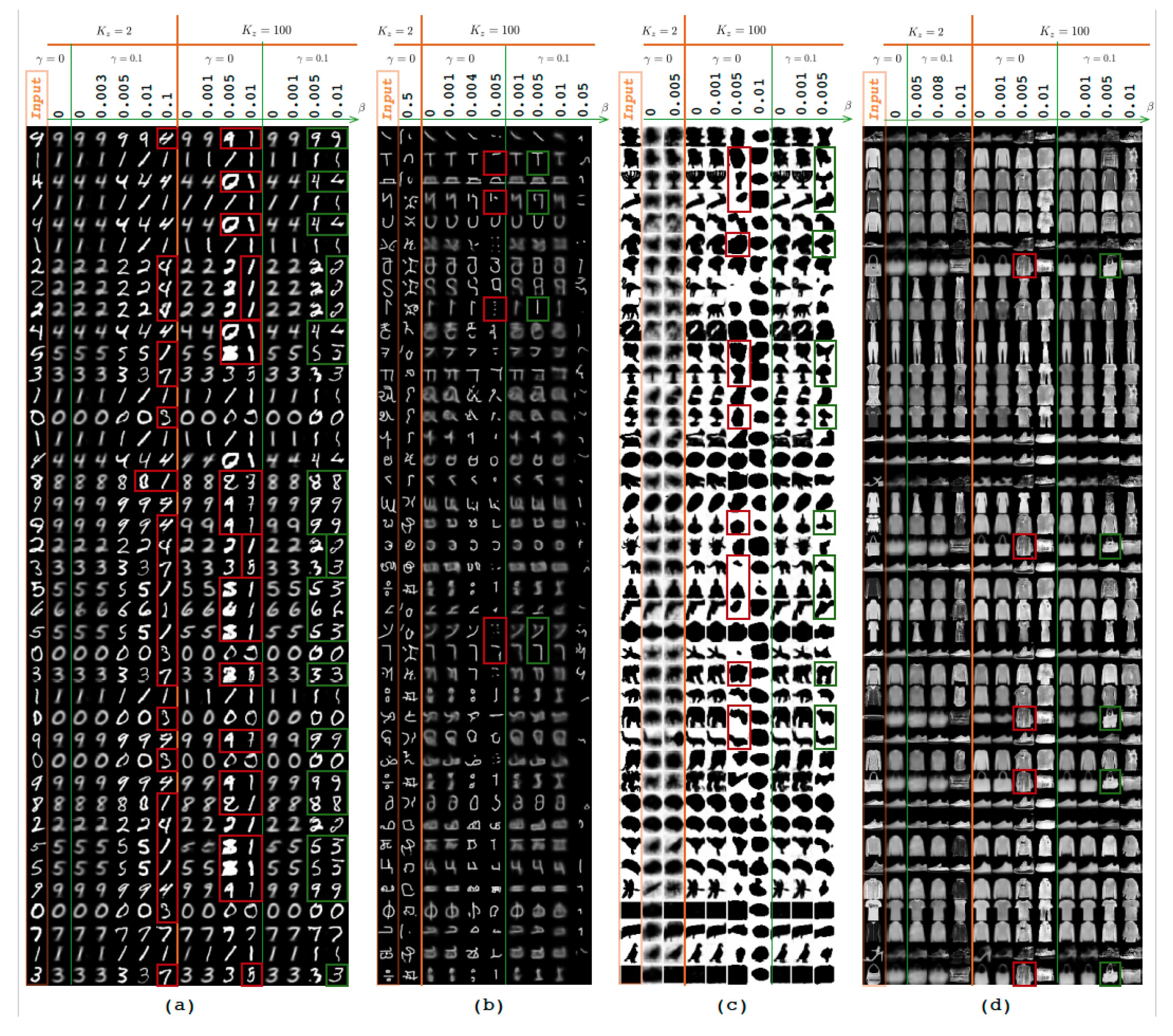
Figure 9 gives all the results obtained for the four databases with different values of and for each of the two latent spaces ( and ). For every database, we randomly generated 40 images as inputs of the VAE. The resulting output image is given according to the experimental parameters.
A. Impact of the latent space: The first observation that can be extracted from these tests concerns the influence of the latent space size on the quality of the reconstructed image. We can see that for the two databases Mnist and Fashion-MNIST, the results achieved on the two-dimensional latent space are almost as good as for . Nevertheless the quality of the reconstruction alone, obtained by setting the adversary parameter , is better for : the images are less blurred and close to the input image than on the 2D latent space.
On the other hand, the image reconstruction performance obtained on the 2D space is less convincing for the Caltech database. Indeed, we can see that the reconstructed images are very blurred but for the most part close to the original image. Note that the reconstruction was completely impossible for the Omniglot database in 2D space. The only result in this space was obtained by forcing the weight of the adversary loss to 0.5, which allowed to generate new world alphabets.
B. Impact of the parameter: In order to measure the effect of adversarial loss term on the feature reconstruction loss term , we varied the adversarial parameter during each test sequence in a progressive way. This test allows to evaluate how the data generation effect can affect the reconstruction effect. Generally speaking, we obtain three steps, which are described as follows:
- dominant reconstruction effect with blurred images.
- reconstruction effect with clearer and more realistic images.
- generative effect is dominant.
with and are two thresholds to define. This is clearly illustrated by the MNIST database. Let us take the case of :
- Up to , the reconstruction effect is dominant with blurred images.
- For the images are clearer and more realistic.
- The generative effect becomes dominant for where most of the resulting images do not match the original ones. These cases are highlighted in red.
C. Impact of the parameter: In order to avoid the generative effect from becoming stronger than the reconstruction one and thus to limit the dominant effect of adversarial loss term , we have varied the parameter in an increasing way, under two different configurations of ( and ). This measures the effect of the latent loss term . We can see that it had the expected effect. The red-framed images have been corrected and are now compatible with the original images again. These corrected images are framed in green.
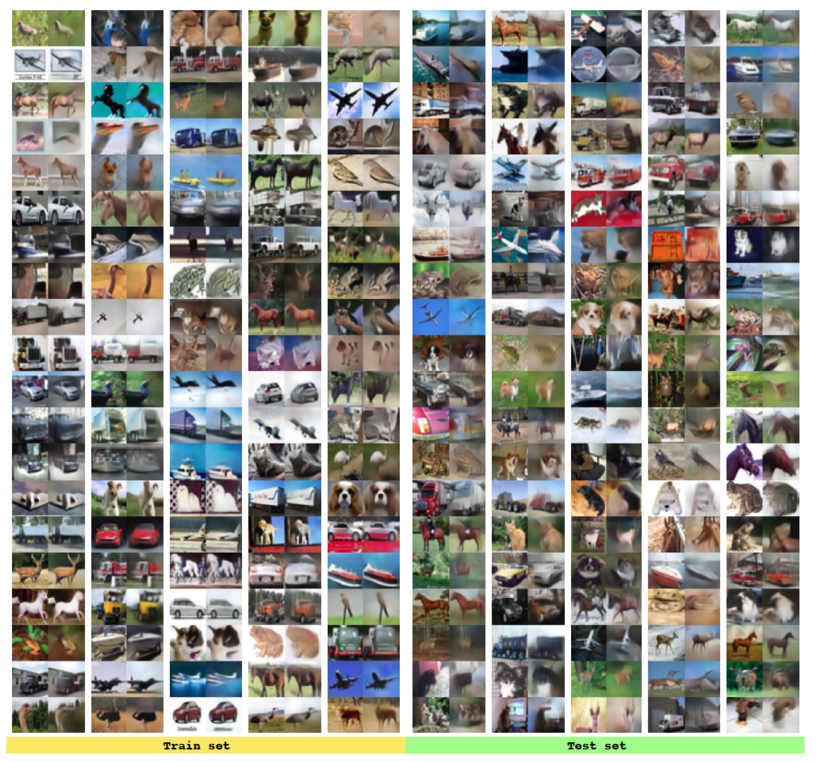
4.5. Test on Cifar 10
5. Conclusions
In this article, we propose a new technique for the training of the varitional autoencoder by incorporating several efficient constraints. Particularly, we use the principle of consistency of deep characteristics to allow the output of the decoder to have a better reconstruction quality. The adversarial constraints allow the decoder to generate data with better authenticity and more realism than the conventional VAE. Finally, by using a two-step learning process, our method can be more widely used in applications other than image processing.
Funding
This research received no external funding.
Conflicts of Interest
The author declares no conflict of interest.
References
- Martin, G.S.; Droguett, E.L.; Meruane, V.; das Chagas Moura, M. Deep variational auto-encoders: A promising tool for dimensionality reduction and ball bearing elements fault diagnosis. Struct. Health Monit. 2018. [Google Scholar] [CrossRef]
- Canchumuni, S.W.; Emerick, A.A.; Pacheco, M.A.C. Towards a robust parameterization for conditioning facies models using deep variational autoencoders and ensemble smoother. Comput. Geosci. 2019, 128, 87–102. [Google Scholar] [CrossRef] [Green Version]
- Lee, S.; Kwak, M.; Tsui, K.L.; Kim, S.B. Process monitoring using variational autoencoder for high-dimensional nonlinear processes. Eng. Appl. Artif. Intell. 2019, 83, 13–27. [Google Scholar] [CrossRef]
- Zhang, Z.; Jiang, T.; Zhan, C.; Yang, Y. Gaussian feature learning based on variational autoencoder for improving nonlinear process monitoring. J. Process. Control. 2019, 75, 136–155. [Google Scholar] [CrossRef]
- Goodfellow, I.; Pouget-Abadie, J.; Mirza, M.; Xu, B.; Warde-Farley, D.; Ozair, S.; Courville, A.; Bengio, Y. Generative Adversarial Nets. In Advances in Neural Information Processing Systems 27; Ghahramani, Z., Welling, M., Cortes, C., Lawrence, N.D., Weinberger, K.Q., Eds.; Curran Associates, Inc.: Montreal, QC, Canada, 2014; pp. 2672–2680. [Google Scholar]
- Yan, S.; Smith, J.S.; Lu, W.; Zhang, B. Abnormal Event Detection from Videos using a Two-stream Recurrent Variational Autoencoder. IEEE Trans. Cogn. Dev. Syst. 2018, 12, 30–42. [Google Scholar] [CrossRef]
- Wang, T.; Qiao, M.; Lin, Z.; Li, C.; Snoussi, H.; Liu, Z.; Choi, C. Generative Neural Networks for Anomaly Detection in Crowded Scenes. IEEE Trans. Inf. Forensics Secur. 2019, 14, 1390–1399. [Google Scholar] [CrossRef]
- Sun, J.; Wang, X.; Xiong, N.; Shao, J. Learning Sparse Representation With Variational Auto-Encoder for Anomaly Detection. IEEE Access 2018, 6, 33353–33361. [Google Scholar] [CrossRef]
- He, M.; Meng, Q.; Zhang, S. Collaborative Additional Variational Autoencoder for Top-N Recommender Systems. IEEE Access 2019, 7, 5707–5713. [Google Scholar] [CrossRef]
- Xu, W.; Tan, Y. Semisupervised Text Classification by Variational Autoencoder. IEEE Trans. Neural Netw. Learn. Syst. 2019, 31, 295–308. [Google Scholar] [CrossRef]
- Song, T.; Sun, J.; Chen, B.; Peng, W.; Song, J. Latent Space Expanded Variational Autoencoder for Sentence Generation. IEEE Access 2019, 7, 144618–144627. [Google Scholar] [CrossRef]
- Wang, X.; Takaki, S.; Yamagishi, J.; King, S.; Tokuda, K. A Vector Quantized Variational Autoencoder (VQ-VAE) Autoregressive Neural F0 Model for Statistical Parametric Speech Synthesis. IEEE/ACM Trans. Audio Speech Lang. Process. 2019, 28, 157–170. [Google Scholar] [CrossRef]
- Agrawal, P.; Ganapathy, S. Modulation Filter Learning Using Deep Variational Networks for Robust Speech Recognition. IEEE J. Sel. Top. Signal Process. 2019, 13, 244–253. [Google Scholar] [CrossRef]
- Kameoka, H.; Kaneko, T.; Tanaka, K.; Hojo, N. ACVAE-VC: Non-Parallel Voice Conversion With Auxiliary Classifier Variational Autoencoder. IEEE/ACM Trans. Audio Speech Lang. Process. 2019, 27, 1432–1443. [Google Scholar] [CrossRef]
- Khodayar, M.; Mohammadi, S.; Khodayar, M.E.; Wang, J.; Liu, G. Convolutional Graph Autoencoder: A Generative Deep Neural Network for Probabilistic Spatio-temporal Solar Irradiance Forecasting. IEEE Trans. Sustain. Energy 2019, 11, 571–583. [Google Scholar] [CrossRef]
- Deng, X.; Huangfu, F. Collaborative Variational Deep Learning for Healthcare Recommendation. IEEE Access 2019, 7, 55679–55688. [Google Scholar] [CrossRef]
- Han, K.; Wen, H.; Shi, J.; Lu, K.H.; Zhang, Y.; Fu, D.; Liu, Z. Variational autoencoder: An unsupervised model for encoding and decoding fMRI activity in visual cortex. NeuroImage 2019, 198, 125–136. [Google Scholar] [CrossRef]
- Bi, L.; Zhang, J.; Lian, J. EEG-Based Adaptive Driver-Vehicle Interface Using Variational Autoencoder and PI-TSVM. IEEE Trans. Neural Syst. Rehabil. Eng. 2019, 27, 2025–2033. [Google Scholar] [CrossRef]
- Wang, D.; Gu, J. VASC: Dimension Reduction and Visualization of Single-cell RNA-seq Data by Deep Variational Autoencoder. Genom. Proteom. Bioinform. 2018, 16, 320–331, Bioinformatics Commons (II). [Google Scholar] [CrossRef]
- Zemouri, R.; Lévesque, M.; Amyot, N.; Hudon, C.; Kokoko, O.; Tahan, S.A. Deep Convolutional Variational Autoencoder as a 2D-Visualization Tool for Partial Discharge Source Classification in Hydrogenerators. IEEE Access 2020, 8, 5438–5454. [Google Scholar] [CrossRef]
- Na, J.; Jeon, K.; Lee, W.B. Toxic gas release modeling for real-time analysis using variational autoencoder with convolutional neural networks. Chem. Eng. Sci. 2018, 181, 68–78. [Google Scholar] [CrossRef]
- Li, H.; Misra, S. Prediction of Subsurface NMR T2 Distributions in a Shale Petroleum System Using Variational Autoencoder-Based Neural Networks. IEEE Geosci. Remote Sens. Lett. 2017, 14, 2395–2397. [Google Scholar] [CrossRef]
- Huang, Y.; Chen, C.; Huang, C. Motor Fault Detection and Feature Extraction Using RNN-Based Variational Autoencoder. IEEE Access 2019, 7, 139086–139096. [Google Scholar] [CrossRef]
- Wang, K.; Forbes, M.G.; Gopaluni, B.; Chen, J.; Song, Z. Systematic Development of a New Variational Autoencoder Model Based on Uncertain Data for Monitoring Nonlinear Processes. IEEE Access 2019, 7, 22554–22565. [Google Scholar] [CrossRef]
- Cheng, F.; He, Q.P.; Zhao, J. A novel process monitoring approach based on variational recurrent autoencoder. Comput. Chem. Eng. 2019, 129, 106515. [Google Scholar] [CrossRef]
- Creswell, A.; White, T.; Dumoulin, V.; Arulkumaran, K.; Sengupta, B.; Bharath, A.A. Generative Adversarial Networks: An Overview. IEEE Signal Process. Mag. 2018, 35, 53–65. [Google Scholar] [CrossRef] [Green Version]
- Zemouri, R.; Zerhouni, N.; Racoceanu, D. Deep Learning in the Biomedical Applications: Recent and Future Status. Appl. Sci. 2019, 9, 1526. [Google Scholar] [CrossRef] [Green Version]
- Wang, Z.; Wang, J.; Wang, Y. An intelligent diagnosis scheme based on generative adversarial learning deep neural networks and its application to planetary gearbox fault pattern recognition. Neurocomputing 2018, 310, 213–222. [Google Scholar] [CrossRef]
- Wang, X.; Huang, H.; Hu, Y.; Yang, Y. Partial Discharge Pattern Recognition with Data Augmentation based on Generative Adversarial Networks. In Proceedings of the 2018 Condition Monitoring and Diagnosis (CMD), Perth, WA, Australia, 23–26 September 2018; pp. 1–4. [Google Scholar] [CrossRef]
- Liu, H.; Zhou, J.; Xu, Y.; Zheng, Y.; Peng, X.; Jiang, W. Unsupervised fault diagnosis of rolling bearings using a deep neural network based on generative adversarial networks. Neurocomputing 2018, 315, 412–424. [Google Scholar] [CrossRef]
- Mao, W.; Liu, Y.; Ding, L.; Li, Y. Imbalanced Fault Diagnosis of Rolling Bearing Based on Generative Adversarial Network: A Comparative Study. IEEE Access 2019, 7, 9515–9530. [Google Scholar] [CrossRef]
- Shao, S.; Wang, P.; Yan, R. Generative adversarial networks for data augmentation in machine fault diagnosis. Comput. Ind. 2019, 106, 85–93. [Google Scholar] [CrossRef]
- Han, T.; Liu, C.; Yang, W.; Jiang, D. A novel adversarial learning framework in deep convolutional neural network for intelligent diagnosis of mechanical faults. Knowl. Based Syst. 2019, 165, 474–487. [Google Scholar] [CrossRef]
- Alam, M.; Vidyaratne, L.; Iftekharuddin, K. Novel deep generative simultaneous recurrent model for efficient representation learning. Neural Netw. 2018, 107, 12–22, Special issue on deep reinforcement learning. [Google Scholar] [CrossRef] [PubMed]
- Zhu, J.Y.; Park, T.; Isola, P.; Efros, A.A. Unpaired Image-to-Image Translation using Cycle-Consistent Adversarial Networks. In Proceedings of the 2017 IEEE International Conference on Computer Vision (ICCV), Venice, Italy, 22–29 October 2017. [Google Scholar]
- Yi, Z.; Zhang, H.; Tan, P.; Gong, M. DualGAN: Unsupervised Dual Learning for Image-to-Image Translation. In Proceedings of the 2017 IEEE International Conference on Computer Vision (ICCV), Venice, Italy, 22–29 October 2017. [Google Scholar]
- Pathak, D.; Krahenbuhl, P.; Donahue, J.; Darrell, T.; Efros, A.A. Context Encoders: Feature Learning by Inpainting. In Proceedings of the 2016 IEEE Conference on Computer Vision and Pattern Recognition (CVPR), Las Vegas, NV, USA, 27–30 June 2016. [Google Scholar]
- Odena, A.; Olah, C.; Shlens, J. Conditional Image Synthesis With Auxiliary Classifier GANs. arXiv 2016, arXiv:stat.ML/1610.09585. [Google Scholar]
- Odena, A. Semi-Supervised Learning with Generative Adversarial Networks. arXiv 2016, arXiv:stat.ML/1606.01583. [Google Scholar]
- Mirza, M.; Osindero, S. Conditional Generative Adversarial Nets. arXiv 2014, arXiv:cs.LG/1411.1784. [Google Scholar]
- Mao, X.; Li, Q.; Xie, H.; Lau, R.Y.K.; Wang, Z.; Smolley, S.P. Least Squares Generative Adversarial Networks. arXiv 2016, arXiv:cs.CV/1611.04076. [Google Scholar]
- Liu, M.Y.; Tuzel, O. Coupled Generative Adversarial Networks. arXiv 2016, arXiv:cs.CV/1606.07536. [Google Scholar]
- Ledig, C.; Theis, L.; Huszar, F.; Caballero, J.; Cunningham, A.; Acosta, A.; Aitken, A.; Tejani, A.; Totz, J.; Wang, Z.; et al. Photo-Realistic Single Image Super-Resolution Using a Generative Adversarial Network. arXiv 2016, arXiv:cs.CV/1609.04802. [Google Scholar]
- Kim, T.; Cha, M.; Kim, H.; Lee, J.K.; Kim, J. Learning to Discover Cross-Domain Relations with Generative Adversarial Networks. arXiv 2017, arXiv:cs.CV/1703.05192. [Google Scholar]
- Isola, P.; Zhu, J.Y.; Zhou, T.; Efros, A.A. Image-to-Image Translation with Conditional Adversarial Networks. arXiv 2016, arXiv:cs.CV/1611.07004. [Google Scholar]
- Hjelm, R.D.; Jacob, A.P.; Che, T.; Trischler, A.; Cho, K.; Bengio, Y. Boundary-Seeking Generative Adversarial Networks. arXiv 2017, arXiv:stat.ML/1702.08431. [Google Scholar]
- Arjovsky, M.; Chintala, S.; Bottou, L. Wasserstein GAN. arXiv 2017, arXiv:stat.ML/1701.07875. [Google Scholar]
- Donahue, J.; Krähenbühl, P.; Darrell, T. Adversarial Feature Learning. arXiv 2016, arXiv:cs.LG/1605.09782. [Google Scholar]
- Denton, E.; Gross, S.; Fergus, R. Semi-Supervised Learning with Context-Conditional Generative Adversarial Networks. arXiv 2016, arXiv:cs.CV/1611.06430. [Google Scholar]
- Chen, X.; Duan, Y.; Houthooft, R.; Schulman, J.; Sutskever, I.; Abbeel, P. InfoGAN: Interpretable Representation Learning by Information Maximizing Generative Adversarial Nets. arXiv 2016, arXiv:cs.LG/1606.03657. [Google Scholar]
- Bousmalis, K.; Silberman, N.; Dohan, D.; Erhan, D.; Krishnan, D. Unsupervised Pixel-Level Domain Adaptation with Generative Adversarial Networks. arXiv 2016, arXiv:cs.CV/1612.05424. [Google Scholar]
- Dumoulin, V.; Belghazi, I.; Poole, B.; Mastropietro, O.; Lamb, A.; Arjovsky, M.; Courville, A. Adversarially Learned Inference. arXiv 2016, arXiv:stat.ML/1606.00704. [Google Scholar]
- Makhzani, A.; Shlens, J.; Jaitly, N.; Goodfellow, I.; Frey, B. Adversarial Autoencoders. arXiv 2015, arXiv:cs.LG/1511.05644. [Google Scholar]
- Hou, X.; Sun, K.; Shen, L.; Qiu, G. Improving variational autoencoder with deep feature consistent and generative adversarial training. Neurocomputing 2019, 341, 183–194. [Google Scholar] [CrossRef] [Green Version]
- Hwang, U.; Park, J.; Jang, H.; Yoon, S.; Cho, N.I. PuVAE: A Variational Autoencoder to Purify Adversarial Examples. IEEE Access 2019, 7, 126582–126593. [Google Scholar] [CrossRef]
- Gatys, L.A.; Ecker, A.S.; Bethge, M. A Neural Algorithm of Artistic Style. arXiv 2015, arXiv:1508.06576. [Google Scholar] [CrossRef]
- Simonyan, K.; Zisserman, A. Very Deep Convolutional Networks for Large-Scale Image Recognition. arXiv 2014, arXiv:1409.1556. [Google Scholar]
- Yu, S.; Príncipe, J.C. Understanding autoencoders with information theoretic concepts. Neural Netw. 2019, 117, 104–123. [Google Scholar] [CrossRef] [PubMed] [Green Version]
- Bengio, Y. How Auto-Encoders Could Provide Credit Assignment in Deep Networks via Target Propagation. arXiv 2014, arXiv:1407.7906. [Google Scholar]
- Im, D.J.; Ahn, S.; Memisevic, R.; Bengio, Y. Denoising Criterion for Variational Auto-Encoding Framework. arXiv 2015, arXiv:1511.06406. [Google Scholar]
- Fan, Y.J. Autoencoder node saliency: Selecting relevant latent representations. Pattern Recognit. 2019, 88, 643–653. [Google Scholar] [CrossRef] [Green Version]
- Kingma, D.P.; Welling, M. Auto-Encoding Variational Bayes. arXiv 2013, arXiv:1312.6114. [Google Scholar]
- Kingma, D. Variational Inference & Deep Learning: A New Synthesis. Ph.D. Thesis, Faculty of Science (FNWI), Informatics Institute (IVI), University of Amsterdam, Amsterdam, The Netherlands, 2017. [Google Scholar]
- Blei, D.M.; Kucukelbir, A.; McAuliffe, J.D. Variational Inference: A Review for Statisticians. arXiv 2016, arXiv:1601.00670. [Google Scholar] [CrossRef] [Green Version]
- Lin, T.; Dollár, P.; Girshick, R.B.; He, K.; Hariharan, B.; Belongie, S.J. Feature Pyramid Networks for Object Detection. arXiv 2016, arXiv:1612.03144. [Google Scholar]
- Zemouri, R.; Devalland, C.; Valmary-Degano, S.; Zerhouni, N. Intelligence artificielle: Quel avenir en anatomie pathologique? Ann. Pathol. 2019, 39, 119–129, L’anatomopathologie augmentée. [Google Scholar] [CrossRef]
- Lecun, Y.; Bottou, L.; Bengio, Y.; Haffner, P. Gradient-based learning applied to document recognition. Proc. IEEE 1998, 86, 2278–2324. [Google Scholar] [CrossRef] [Green Version]
- Lake, B.M.; Salakhutdinov, R.R.; Tenenbaum, J. One-shot learning by inverting a compositional causal process. In Advances in Neural Information Processing Systems 26; Burges, C.J.C., Bottou, L., Welling, M., Ghahramani, Z., Weinberger, K.Q., Eds.; Curran Associates, Inc.: Lake Tahoe, NV, USA, 2013; pp. 2526–2534. [Google Scholar]
- Marlin, B.; Swersky, K.; Chen, B.; Freitas, N. Inductive Principles for Restricted Boltzmann Machine Learning. In Machine Learning Research, Proceedings of the Thirteenth International Conference on Artificial Intelligence and Statistics, Sardinia, Italy, 13–15 May 2010; PMLR: Chia Laguna Resort; Teh, Y.W., Titterington, M., Eds.; GitHub: San Francisco, CA, USA, 2010; Volume 9, pp. 509–516. [Google Scholar]
- Xiao, H.; Rasul, K.; Vollgraf, R. Fashion-MNIST: A Novel Image Dataset for Benchmarking Machine Learning Algorithms. arXiv 2017, arXiv:1708.07747. [Google Scholar]
- Krizhevsky, A.; Hinton, G. Learning Multiple Layers of Features from Tiny Images. Master’s Thesis, Department of Computer Science, University of Toronto, Toronto, ON, Canada, 2009. [Google Scholar]
Figure 1.
Schematic architecture of a standard deep autoencoder and a variational deep autoencoder. Both architectures have two parts: an encoder and a decoder.
Figure 1.
Schematic architecture of a standard deep autoencoder and a variational deep autoencoder. Both architectures have two parts: an encoder and a decoder.

Figure 2.
Illustration of the generative adversarial network (GAN).

Figure 3.
The framework of the proposed method.

Figure 4.
Deep feature consistent.

Figure 5.
Random example images from the dataset; (a) MNIST, (b) Omniglot, (c) Caltech 101 Silhouettes, (d) Fashion MNIST.
Figure 5.
Random example images from the dataset; (a) MNIST, (b) Omniglot, (c) Caltech 101 Silhouettes, (d) Fashion MNIST.

Figure 6.
The architecture of the encoder, decoder, discriminator and the classifier.

Figure 7.
The 2D latent space obtained for the four databases; (a) MNIST, (b) Omniglot, (c) Caltech 101 Silhouettes, (d) Fashion MNIST.
Figure 7.
The 2D latent space obtained for the four databases; (a) MNIST, (b) Omniglot, (c) Caltech 101 Silhouettes, (d) Fashion MNIST.

Figure 8.
Images generated from the latent space for the (a) Mnist and (b) the Fashion Mnist.

Figure 9.
The results obtained for the four databases with different values of and for each of the two latent spaces ( and ); (a) MNIST, (b) Omniglot, (c) Caltech 101 Silhouettes, (d) Fashion MNIST.
Figure 9.
The results obtained for the four databases with different values of and for each of the two latent spaces ( and ); (a) MNIST, (b) Omniglot, (c) Caltech 101 Silhouettes, (d) Fashion MNIST.

Figure 10.
Several pairs of random images with their reconstructed output of the CIFAR10.

© 2020 by the author. Licensee MDPI, Basel, Switzerland. This article is an open access article distributed under the terms and conditions of the Creative Commons Attribution (CC BY) license (http://creativecommons.org/licenses/by/4.0/).
Share and Cite
MDPI and ACS Style
Zemouri, R. Semi-Supervised Adversarial Variational Autoencoder. Mach. Learn. Knowl. Extr. 2020, 2, 361-378. https://0-doi-org.brum.beds.ac.uk/10.3390/make2030020
AMA Style
Zemouri R. Semi-Supervised Adversarial Variational Autoencoder. Machine Learning and Knowledge Extraction. 2020; 2(3):361-378. https://0-doi-org.brum.beds.ac.uk/10.3390/make2030020
Chicago/Turabian StyleZemouri, Ryad. 2020. "Semi-Supervised Adversarial Variational Autoencoder" Machine Learning and Knowledge Extraction 2, no. 3: 361-378. https://0-doi-org.brum.beds.ac.uk/10.3390/make2030020