Article

Learning DOM Trees of Web Pages by Subpath Kernel and Detecting Fake e-Commerce Sites

1
Computer Centre, Gakushuin University, Tokyo 1718588, Japan
2
Information Networking Institute, Carnegie Mellon University, Pittsburgh, PA 15213, USA
3
Cyber Security Defense Department, Rakuten, Inc., Tokyo 1580094, Japan
4
Data Engineering, Evidation Health, Inc., San Mateo, CA 94402, USA
*
Author to whom correspondence should be addressed.
Current address: 1-5-1 Mejiro, Toshima, Tokyo 1718588, Japan.
Mach. Learn. Knowl. Extr. 2021, 3(1), 95-122; https://0-doi-org.brum.beds.ac.uk/10.3390/make3010006
Submission received: 9 December 2020 / Revised: 29 December 2020 / Accepted: 10 January 2021 / Published: 14 January 2021
(This article belongs to the Special Issue Selected Papers from CD-MAKE 2020 and ARES 2020)

Abstract

:
The subpath kernel is a class of positive definite kernels defined over trees, which has the following advantages for the purposes of classification, regression and clustering: it can be incorporated into a variety of powerful kernel machines including SVM; It is invariant whether input trees are ordered or unordered; It can be computed by significantly fast linear-time algorithms; And, finally, its excellent learning performance has been proven through intensive experiments in the literature. In this paper, we leverage recent advances in tree kernels to solve real problems. As an example, we apply our method to the problem of detecting fake e-commerce sites. Although the problem is similar to phishing site detection, the fact that mimicking existing authentic sites is harmful for fake e-commerce sites marks a clear difference between these two problems. We focus on fake e-commerce site detection for three reasons: e-commerce fraud is a real problem that companies and law enforcement have been cooperating to solve; Inefficiency hampers existing approaches because datasets tend to be large, while subpath kernel learning overcomes these performance challenges; And we offer increased resiliency against attempts to subvert existing detection methods through incorporating robust features that adversaries cannot change: the DOM-trees of web-sites. Our real-world results are remarkable: our method has exhibited accuracy as high as 0.998 when training SVM with 1000 instances and evaluating accuracy for almost 7000 independent instances. Its generalization efficiency is also excellent: with only 100 training instances, the accuracy score reached 0.996.

1. Introduction

Tree-structured data has been the focus of a great deal of machine learning research for a long time. In 1979, Taï [1] extended Levenshtein edit distance [2] to trees, and since then, we have been able to use distance measures to evaluate the similarity of trees. In 2001, Collins and Duffy [3] introduced the first instance of tree kernels and has opened new avenues for leveraging a variety of powerful kernel machines to study trees. Furthermore, recent work has shown that the subpath kernel is both more efficient and accurate than other tree kernels: significantly fast algorithms that compute the subpath kernel in time linear to the size of input trees (the number of vertices) have been proposed [4,5]; An intensive experiment with various datasets has showed that the subpath kernel outperforms other tree kernels in classification accuracy when used with SVM.
Thus, the recent advances in tree kernel methods have made it possible to leverage powerful kernel machines for the purpose of analyzing various real tree data. Two of the most important advantages of using kernel machines are the wide variety of methods based on multivariate analysis, and the excellent generalization performance obtained even when analyzing small datasets. In this regard, the main aims of this paper are to introduce:
  • A generic system design for effective and efficient analysis of tree data with the subpath kernel;
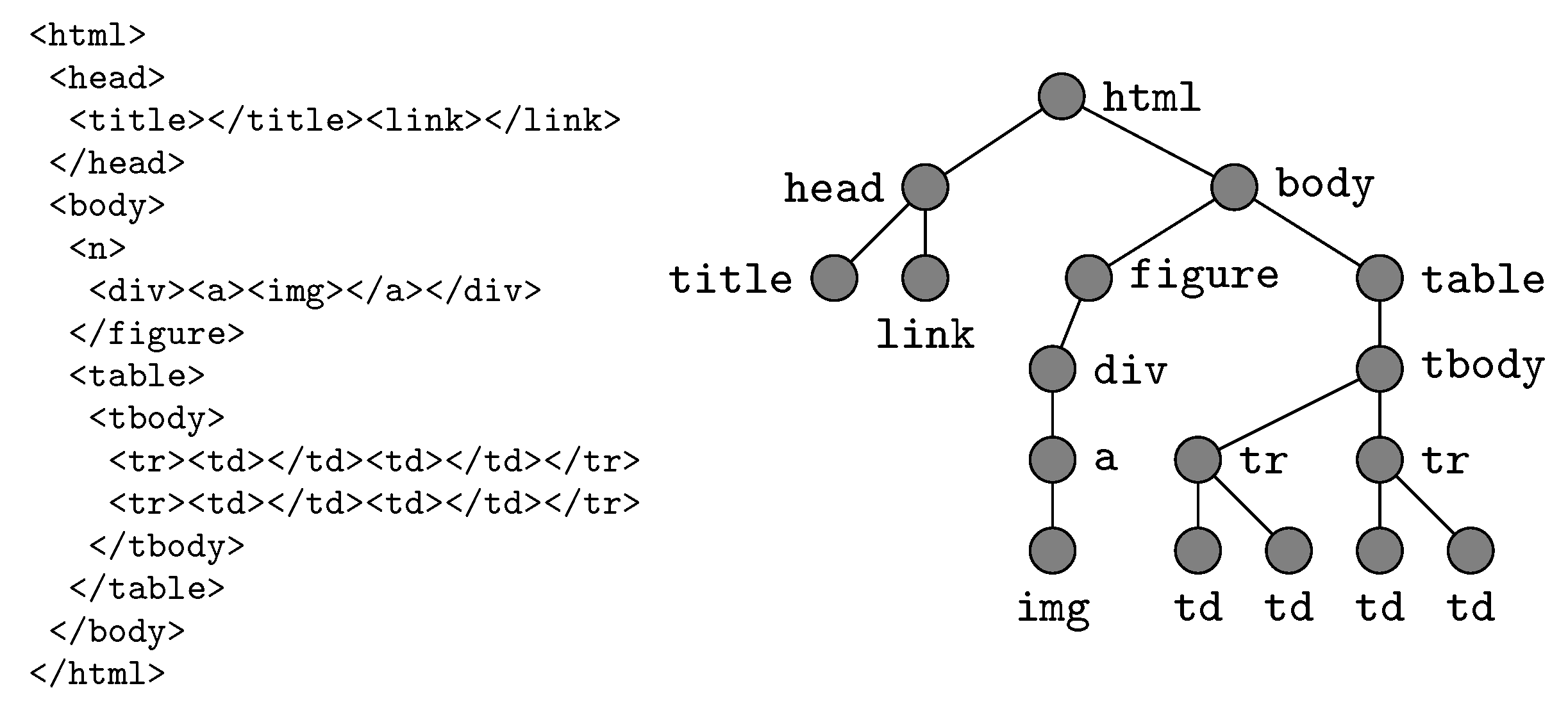
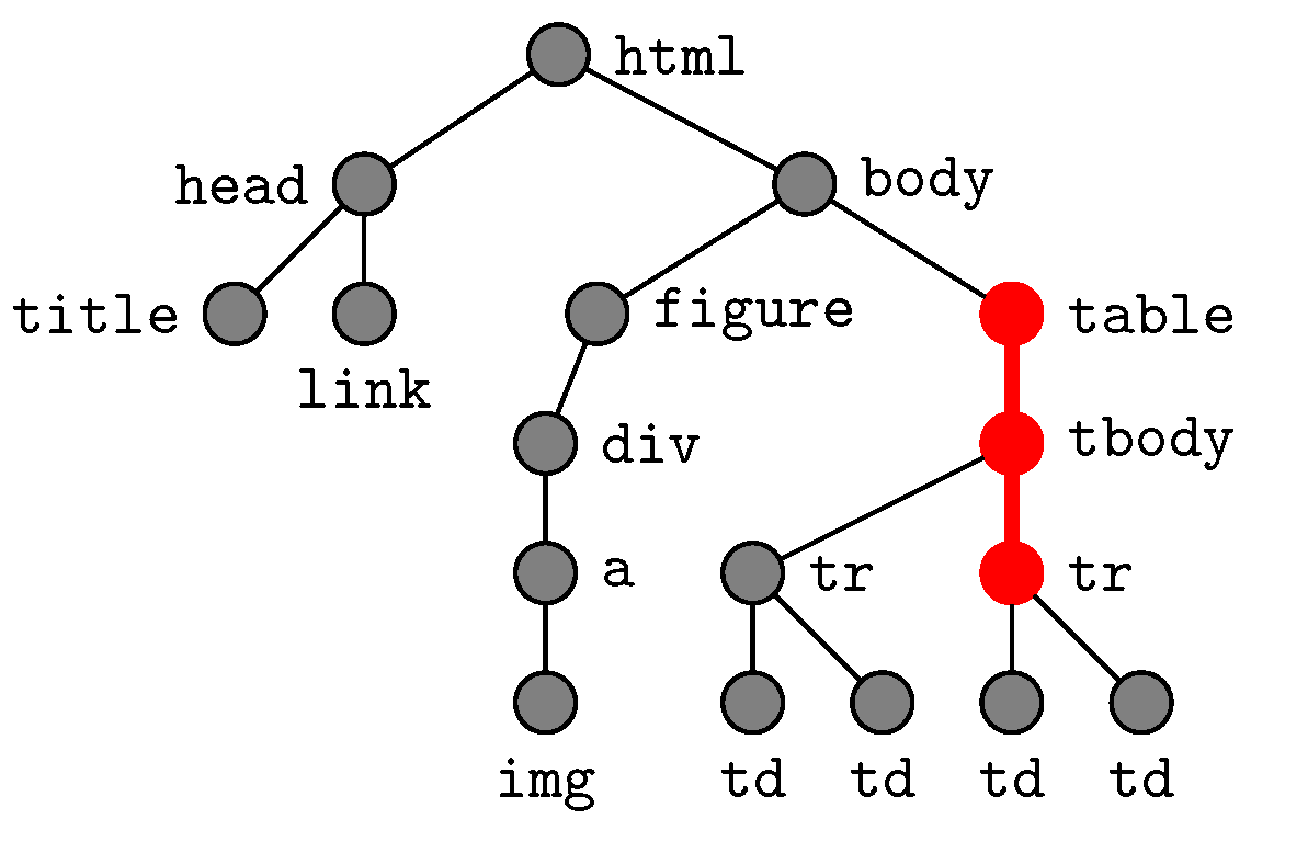
  • A detailed application of the subpath kernel to document object model (DOM) trees, an important example of tree data; and
  • The remarkably high performance observed in analysis of DOM trees for detecting fake e-commerce sites with the subpath kernel system.
Fake e-commerce sites have been serious threats to costumers and providers of e-commerce. They pretend to be authentic sites that are authorized by companies operating e-commerce platforms and attempt to obtain money by fraud, steal personal information such as credit card numbers, ruin reputation of the platform operators, and so forth. The number of reported incidents of fake e-commerce sites started to increase in 2012, and it continues to increase rapidly. In Japan, the monetary damage reported in 2012 was merely 48 million JPY, but rapidly grew to 2.9 billion JPY in 2014 and 3.1 billion JPY in 2015.
Although fake e-commerce sites may seem akin to a popular class of malicious sites referred to as phishing sites, there is a crucial difference. Phishing pages attempt to resemble a single legitimate site, meaning they must mimic one particular site as closely as possible. By contrast, fake e-commerce sites do not have any specific targets, and similarity to specific existing authentic sites is even harmful for them, because the similarity may raise consumers’ awareness of their illegality and as a result will shorten their lifetime. Therefore, phishing detection approaches do not work with e-commerce fraud detection sites, because they cannot be compared to a single known-good target site [6].
Nevertheless, it will be helpful to review the techniques developed for phishing detection. Surveys in the literature (e.g., [7,8,9,10]) have reported that the major sources of information consist of web-page contents, URLs of websites and blacklists.
  • Web-page contents can provide information at the finest granularity, and the range of features that can be extracted is the widest. The features of hyperlinked URLs [11], linked images [11,12], and embedded executable codes [13] are all extracted from page contents. Distributions of various information such as terms used [14], tag contents [11], contents types [14] and terms’ TF-IDF values [15,16] are also useful features. In exchange, the detailed investigation of web-page contents may cause damages to users’ computers by executing malware included, and features extracted from texts are prone to be language-specific. More importantly, content-based features can be shallow in many cases, that is, it is not difficult for adversaries to alter them so as to circumvent detection.
  • The URL of a website can also provide useful information for phishing detection. The features include not only tokens from the URL [15,16,17] but also metadata obtained from external sources such as DNS [15], Google PageRank [15] and Amazon Alexa [14]. Because of the limit of the length of URL strings, the information obtained is also limited. Link redirection and change of web-contents can be an effective circumvention method, as well.
  • A blacklist is created in a concentrative manner and specifies URLs of known phishing sites. Since its trustworthiness is high, it is widely used in real services like Google Safe Browsing [18] and eBay Toolbar [7]. Nevertheless, automated crawlers can be easily detected, and also, changing web-contents can easily outdate it. The most significant disadvantage of blacklists is the time difference between discovery of phishing sites and their registration to blacklists. The most significant disadvantage of blacklists is the time difference between discovery of phishing sites and their registration on blacklists.
In this paper, we are interested in methods that can automatically detect newly born (zero-day) fake websites. Therefore, the blacklist approach is out of the scope of this paper. In general, use of machine learning techniques is known effective to detect zero-day attacks, and the survey [19] introduces latest attempts to apply machine learning techniques to the problem of detecting fake websites. Some leverage the remarkable advances of the research on artificial neural networks (ANN) to obtain excellent detection accuracy [20,21,22,23], while some rely on the established methods including SVM, Decision Tree, Random Forest and Gradient Boosting [23,24].
Many of the reported methods that can detect zero-day fake sites show significantly high accuracy rates of detection. For example, the accuracy of 0.999 is reported in [14,15]. They, however, rely on shallow features, such that adversaries can change their values to bypass detection without insuperable difficulties. This is the problem of the existing methods that we recognize and try to solve.
For the purpose, we develop a far more resilient approach. We propose a method that takes advantage of the structural information of a web page’s document object model (DOM) tree. A DOM tree of a web page is a tree that represents the nesting structure of its hypertext markup language (HTML) tags. Figure 1 shows an extremely simple example of an HTML document and the DOM tree that represents it. Real DOM trees usually include thousands of vertices.
This approach is based on a discovery reached through joint investigation with the National Police Agency of Japan and Rakuten Inc., an e-commerce company that is operating the largest e-commerce platform in Japan. Law enforcement agencies and e-commerce companies have been cooperating to identify fake sites as quickly as possible in order to minimize the damages to consumers. They collect information of fake sites through complaint forms and allocate staff to analyze the collected information. Once they discover fake sites, they add their URLs to public blacklists. This initiative has shut down thousands of fake sites, usually very quickly. As a result of this policework, the average lifetime of a fake site is short, and the criminals must continuously develop and release new fake sites quickly. Because of this short lifespan, a single group of criminals must operate make fake sites simultaneously in order to make profits worth the effort required to maintain a set of short-lived sites. Thus, criminals cannot spend much time or effort developing each new site from scratch. On the other hand, they have to make each site look different to fool consumers. Changing content and layout is easy and affordable, but modifying page structure is expensive. Thus, we expect that DOM trees of web-pages can carry effective and sustainable features for the purpose of discriminating fake sites from authentic sites.
Using HTML tags as features for detecting fake websites has been proposed in the literature. For example, the five categories recommended in [25] as important sources of features are: web page text; web page source code; URLs; images; and, linkage, and HTML tags are obtained from source codes of web pages. The tags are, however, used individually, and their structural information is not incorporated into detection of fake websites. In contrast, the method presented in this paper evaluates only the structural information of HTML tags, that is, DOM trees, not the content of web pages, such as texts or images. This does not mean, however, that features obtained from the other sources are useless. As recommended in [25], it is desirable that real fake-website detection tools rely on features from a variety of sources for robust performance, and we recommend including structural features of DOM trees to measure similarity of web pages.
In [26], the relationship between elements of fake-website detection tools and users’ acceptance of the tools is studied. In particular, accuracy and speed are critical for earning users’ acceptance. While structural information includes effective cues that can lead to improvement in accuracy, analyzing structural information is generally costly in time. In this regard, the subpath kernel can satisfy both of the seemingly contradictory requirements of high accuracy and high efficiency. In fact, as we see in Section 5, the accuracy rate observed in our experiments reaches as high as 0.998, and prediction of a single website with a support vector machine (SVM) classifier requires only a few tens of milliseconds.
In addition, because a (positive definite) tree kernel can be viewed as a method to plot trees as points in Euclidean (Hilbert) spaces, the subpath kernel can be combined with a variety of multi-variate analysis methods including SVM, principal component analysis (PCA), multiple regression analysis, and Gaussian process analysis, and we can select the most effective analysis tool according to our objective.
The remainder of this paper is organized as follows. In Section 2, we give a description of the data that we use in our research. In Section 3, we briefly review a theory of similarity measures to evaluate similarity of DOM trees. Section 3.3.2 reviews tree kernels, the class of measures that we use. Section 4 provides a specific description of the subtree kernel. Section 5 describes our method, experiments, and further applications. Although the target application in this paper is detection of fake e-commerce sites, it has larger applications.

2. The Data Used in Our Research

The initial form of the data that we use in our research is a list of URLs of real e-commerce sites annotated relating to whether the sites of the URLs are fake or authentic. We have obtained the data by different means for fake sites and authentic sites.

2.1. Positive Examples—Fake Sites

Rakuten, Inc. has provided us with a list of 3597 URLs of fake sites. Rakuten is a Japanese electronic commerce and Internet company, which operates Rakuten Ichiba, the largest e-commerce platform in Japan. Rakuten is a large target for fraud because it is ranked 14th worldwide in revenue. The fake sites that Rakuten provided claim to be authorized by Rakuten, but try to defraud consumers with low-quality goods, or products that are never delivered.
To confront this threat, Rakuten has formed an Internet patrol team whose mission is to investigate fraudulent sites. Their current method relies on manual investigation, which they would like to improve through automation.

2.2. Negative Examples—Authentic Sites

The number of authentic sites found by the aforementioned investigation is very small compared to the number of fake sites. Therefore, we need to collect a compatible number of URLs of authentic sites to apply machine learning properly. For the purpose, we have developed a crawler program that visits authentic sites by tracing links starting from a Rakuten’s official site, https://ranking.rakuten.co.jp. This method produced 3349 URLs of authentic sites.
We know, however, that the web-pages that this method collects include pages whose purpose is not to sell goods to consumers. For example, our dataset includes Rakuten’s help pages about its e-commerce platform and credit cards. Nevertheless, we decided to use all of these pages for two reasons: first, the positive examples also include non-shopping sites; and second, the percentage of such non-shopping pages is smaller than 1%, so their impact to machine learning analysis is expected to be limited.

2.3. Partition into a Training and Validation Datasets

We have selected 500 fake sites and 500 authentic sites to include in a training dataset, while the remaining 3097 fake sites and 2849 authentic sites are preserved for validation. The training dataset will be used to train classifiers, while the validation dataset will be used to evaluate how well the classifiers have been trained.

3. Similarity Measures for DOM Trees

As described, we expect that DOM trees include features that persist despite adversaries’ efforts to slip past detection attempts. Nevertheless, not all features of DOM trees are appropriate to use for our purpose. In the following, we will describe what features of DOM trees we should leverage in our proposal.

3.1. Measures Based on Shallow Features

Figure 2 shows histograms of the vertex number s ( t ) , the leaf number l ( t ) and the height h ( t ) of DOM trees t in the training dataset: a leaf is a vertex of t with no children; h ( t ) is the length of the longest upward paths from a leaf to the root in t. We can observe that the thresholds of 970, 498 and 23 for s ( t ) , l ( t ) and h ( t ) can separate the distributions of fake and authentic sites clearly, and the accuracy rates reach 0.941, 0.943 and 0.974, respectively.
Despite the high accuracy of the methods, we cannot use them for our purpose, because adversaries can easily change these values by adding dummy tags to HTML documents without altering their logical meaning or layout. It is also important to note that an appropriate detection method must not be affected by these indices. Otherwise, adversaries can lower the effective detection accuracy by equalizing sizes of trees.
One alternative we might consider to evaluate the similarity of trees is the use of edit distances with distance-based classifiers (for example, k-nearest-neighborhood). However, this method also relies on shallow features. The edit distance is a widely used class of dissimilarity measures and has been intensively studied for a long time. The Taï distance [1] is a well-known example, and many variations have been derived from it. Among them, the subpath distance, which is based on subpaths in trees, has proven to be excellent in classification accuracy [27]: a subpath is an upward sequence of one or more contiguous vertices of a tree (Figure 3). When SP ( t ) denotes the entire set of subpaths of a tree t, the following formula defines the distance:
d S P ( t 1 , t 2 ) = | t 1 | + | t 2 | 2 · max { | p | p SP ( t 1 ) SP ( t 2 ) } .
This approach does not meet our purposes because d S P ( t 1 , t 2 ) relies on a single longest subpath shared between t 1 and t 2 . In fact, when t 1 is fake and t 2 is authentic, adversaries can modify only a small portion of t 1 limiting the resulting change to its logical meaning and layout to the minimum so that t 1 and t 2 share a longer path, which results in a decrease of d S P ( t 1 , t 2 ) . Any variations of the Taï distance suffer from the same problem, since they evaluate the similarity only by maximal shared substructures in the same way as the subtree distance.

3.2. Measures Based on Deep Features

In this paper, we pursue measures that evaluate the similarity of the entire spectrum distributions of substructures in trees.
For example, Figure 4 depicts spectrum distributions of SP ( t ) for a fake tree, an authentic tree and a tree whose authenticity is unknown: the x axis represents subpaths that appear in t, while the y axis indicates their occurrence numbers. Whether the third tree is fake or authentic should be determined by to which the unknown spectrum distribution is more similar, the first or the second. As mentioned, the edit distance d S P ( t 1 , t 2 ) leverages only the length of the longest common subpaths that appear in the distributions and ignore the remainder of the spectrum distributions.
In contrast, a similarity measure that we are pursuing should incorporate every local similarity of the distributions into evaluation: the entire set of substructures of a tree t (for example, SP ( t ) ) determines a neighborhood system around vertices of t, and hence, structural information around every vertex definitely affects the entire spectrum distribution; It is difficult for adversaries to intentionally control changes of a spectrum distribution, because every small change of a tree (for example, a substitution, insertion and deletion of a vertex) will spread widely over the distribution.
We can search such measures from tow major categories: divergences and positive definite mapping kernels.
  • Kullback-Leibler divergence is the best known example, but it does not satisfy the axiom of symmetry. The symmetric divergences include Jensen-Shannon divergence, Bhattacharrya distance, Hellinger distance, L p -norm and Brownian distance. Divergences can be used with distance-based classifiers such as the nearest centroid and k-nearest neighborhood algorithms for classification, and k-means and k-memoid algorithms for clustering.
  • A positive definite kernel K : X × X R can be viewed as an inner product operator · , · of some inner product space H [28] (reproducing kernel Hilbert space, RKHS). That is, by some mapping Φ : X H , an element x X can be identified with a vector Φ ( x ) H , and K ( x , y ) = Φ ( x ) , Φ ( y ) holds. In particular, normalization of K ( x , y ) yields the well-known cosine similarity.
    K ( x , y ) K ( x , x ) K ( y , y ) = Φ ( x ) , Φ ( y ) Φ ( x ) Φ ( y ) = cos θ .
    More importantly, by identifying X as a subspace of H , we can extensively apply many useful multivariate analysis techniques to X including PCA for feature extraction, SVM classifier for classification, the kernel k-means algorithm for clustering, and Gaussian process analysis for regression. A positive definite mapping kernel [27], in addition, evaluates spectrum distributions.
Although both divergences and positive definite mapping kernels can be used for our purpose of evaluating the similarity between DOM trees, this paper deploys the latter, since the advantage of multivariate analysis is significant.

3.3. Prior Work on Tree Mapping Kernels

3.3.1. Positive Definite Mapping Kernels

The mapping kernel is a generalization of the well-known convolution kernel [29] and is defined as follows.
For sets x and y, we call a subset μ x × y a mapping from x to y and allocate a set of mappings M x , y to each pair ( x , y ) . Hence, when X denotes a family of sets, we have a mapping system M determined by M = { M x , y ( x , y ) X × X } . Furthermore, we let k : Ω × Ω R be an arbitrary kernel defined over Ω = x X x . Then, the mapping kernel associated with X and k is determined by
K M , k ( x , y ) = μ M x , y ( v , w ) μ k ( v , w ) .
For example, a convolution kernel is a mapping kernel with the setting of M x , y H = { ( v , w ) } v x , w y and is of the form of
K M H , k ( x , y ) = ( v , w ) x × y k ( v , w ) .
Positive definiteness of a kernel allows us to view it as the inner product operator of some inner product space (RKHS). With respect to positive definiteness of mapping kernels, we have
Theorem 1.
(Shin et al. [30].) The following are equivalent.
  • K M , k is positive definite, if k is positive definite.
  • M is transitive, that is, if μ M x , y and ν M y , z , then the composition ν μ is in M x , z .
For more details, refer to Appendix A.

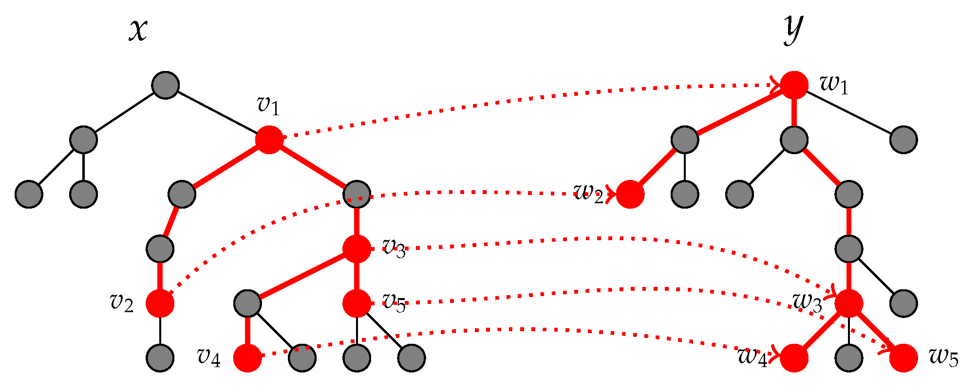
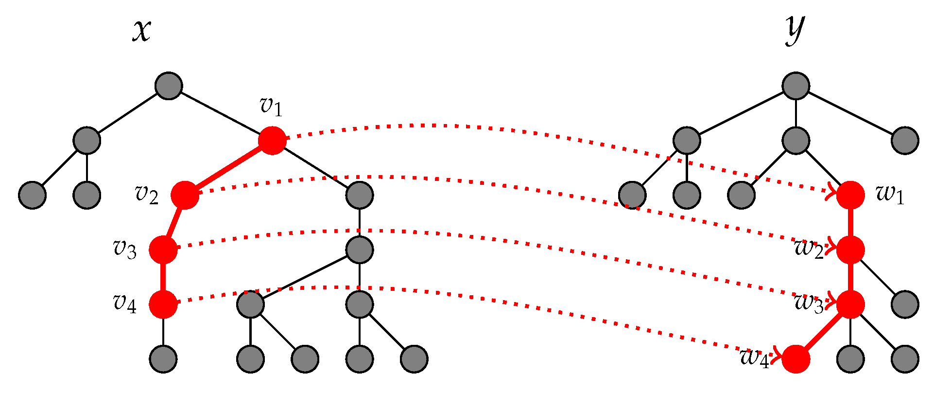
3.3.2. Tree Mapping Kernels

In this paper, a tree always means a rooted ordered tree. A rooted ordered tree is equipped with two orders of vertices: a generation order and a traversal order; A generation order determines an ancestor-to-descendant relation of vertices; v < w indicates that v is an ancestor of w; In particular, v w means that v is the immediate ancestor (parent) of w; The traversal order ≺, on the other hand, determines a left-to-right relation; The nearest common ancestor of v and w is denoted by v w . In Figure 3, for example, html < figure , body figure , head figure and figure tbody = body hold. For a formal description, refer to Appendix B.
Furthermore, we assume the vertices of trees are all labeled: We denote the labeling function by : Ω A , where Ω is the entire set of labeled vertices of our target trees and A is the alphabet of labels.
When x Ω and y Ω represent two trees, a mapping set M x , y to be used for a mapping kernel should be determined so that it reflects the interior structures of x and y. The minimum requirements for μ M x , y are:
  • μ is a one-to-one partial mapping;
  • μ preserves the generation orders of x and y, that is, μ ( v ) < μ ( w ) , if, and only if, v < w ;
  • μ preserves the generation orders of x and y, that is, μ ( v ) μ ( w ) , if, and only if, v w ;
In [31], 32 different mapping systems are defined, and the associated tree mapping kernels are investigated. Among them, we see two examples.
  • The elastic tree kernel [32] is an important example of tree kernels in the literature and is also defined as an instance of mapping kernels with mapping sets M x , y E determined so that μ M x , y E satisfies (1) v w Dom ( μ ) , if { v , w } Dom ( μ ) , and (2) μ ( v w ) = μ ( v ) μ ( w ) . Figure 5 exemplifies μ M x , y E .
  • The subpath kernel [4,33] is also a mapping kernel determined by M x , y SP , which consists of μ x × y such that Dom ( μ ) and Ran ( μ ) are subpaths. Figure 6 exemplifies μ M x , y SP ,
For the interior kernel k : Ω × Ω R to be used in Equation (1), we can use the following kernel with two weight parameters α and β :
k α , β ( v , w ) = ( α β ) δ ( v ) , ( w ) + β = α , if ( v ) = ( w ) ; β , otherwise .
It is easy to see that k α , β is positive definite, if α β 0 . For the elastic and subpath tree kernels, we further constrain β to be zero.

3.3.3. A Comparison of Tree Mapping Kernels

In [31,33], tree mapping kernels obtained from Equations (1) and (2) are comprehensively investigated with respect to the classification accuracy when used with support vector classifiers (SVC). A mapping system M is chosen out of 32 different types including M x , y E and M x , y SP , while ( α , β ) moves over grid points in the region of 0 β α 1 . The comparison is based on averaged ten-fold cross validation scores (accuracy scores) across ten independent datasets.
Figure 7 shows the result of the comparison focusing on the best six tree kernels investigated. For the subpath, parse and elastic tree kernels, β was fixed to zero, while α was adjusted to show the best accuracy performance. For the other kernels, both α and β were adjusted. In the chart, the values in the hatched rectangles show the averaged rank of each kernel, while the figures in parentheses that follow kernel names are p-values of Hommel test [34] as recommendation by [35]. We should remark that the subpath kernel overwhelmingly outperforms the other kernels.

3.4. Conclusion on Kernel Selection

To confirm the superiority of the subpath kernel in classification accuracy, we run an additional experiment using a dataset with 25 fake DOM trees and as many authentic DOM trees. In the experiment, we compare the subpath kernel with 59 tree kernels including the kernels tested in [31,33]. Figure 8 shows the result. The accuracy scores are measured through ten-fold cross validation. Only the subpath kernel marks 1.0 accuracy, while the scores of all the other kernels falls between 0.54 and 0.93. Thus, the subpath kernel outperforms even for the dataset of this paper.
In addition, the subpath kernel has the following advantages.
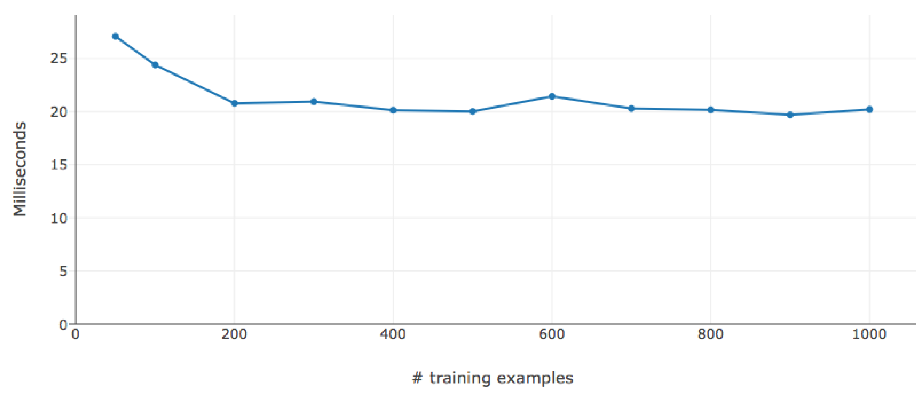
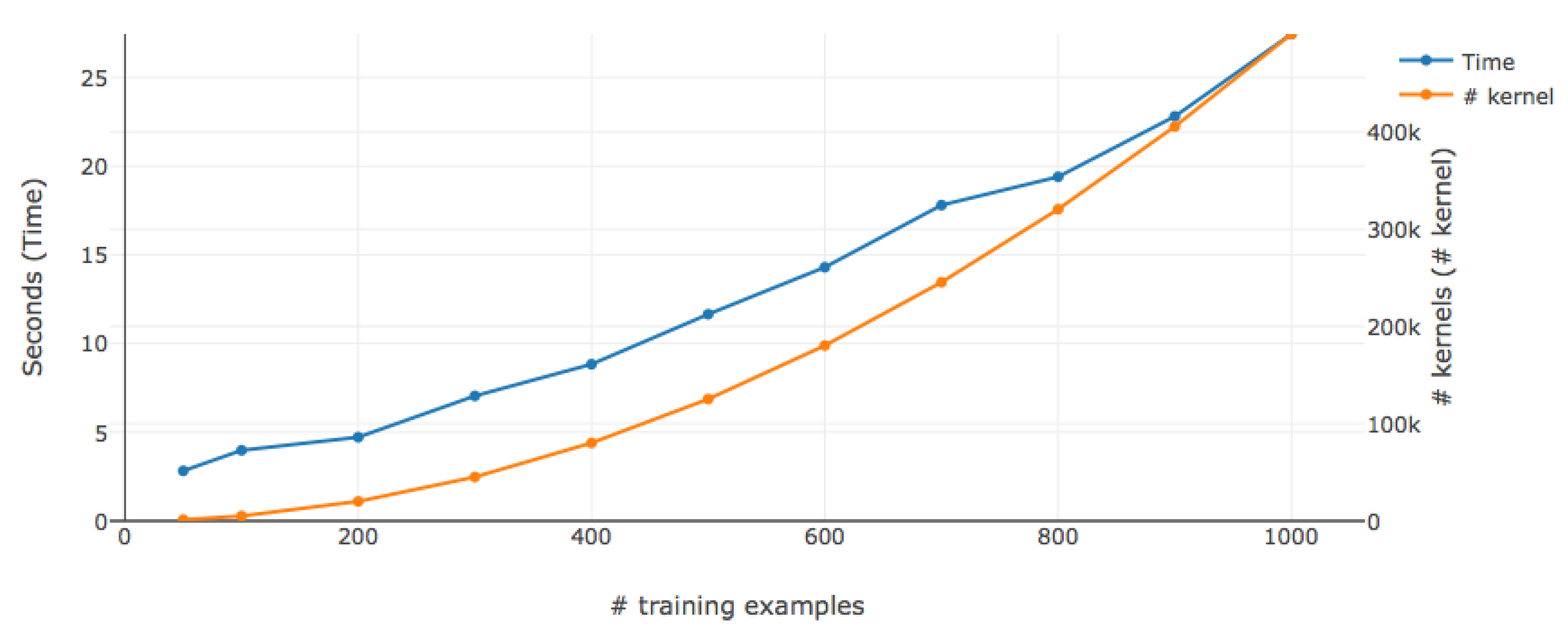
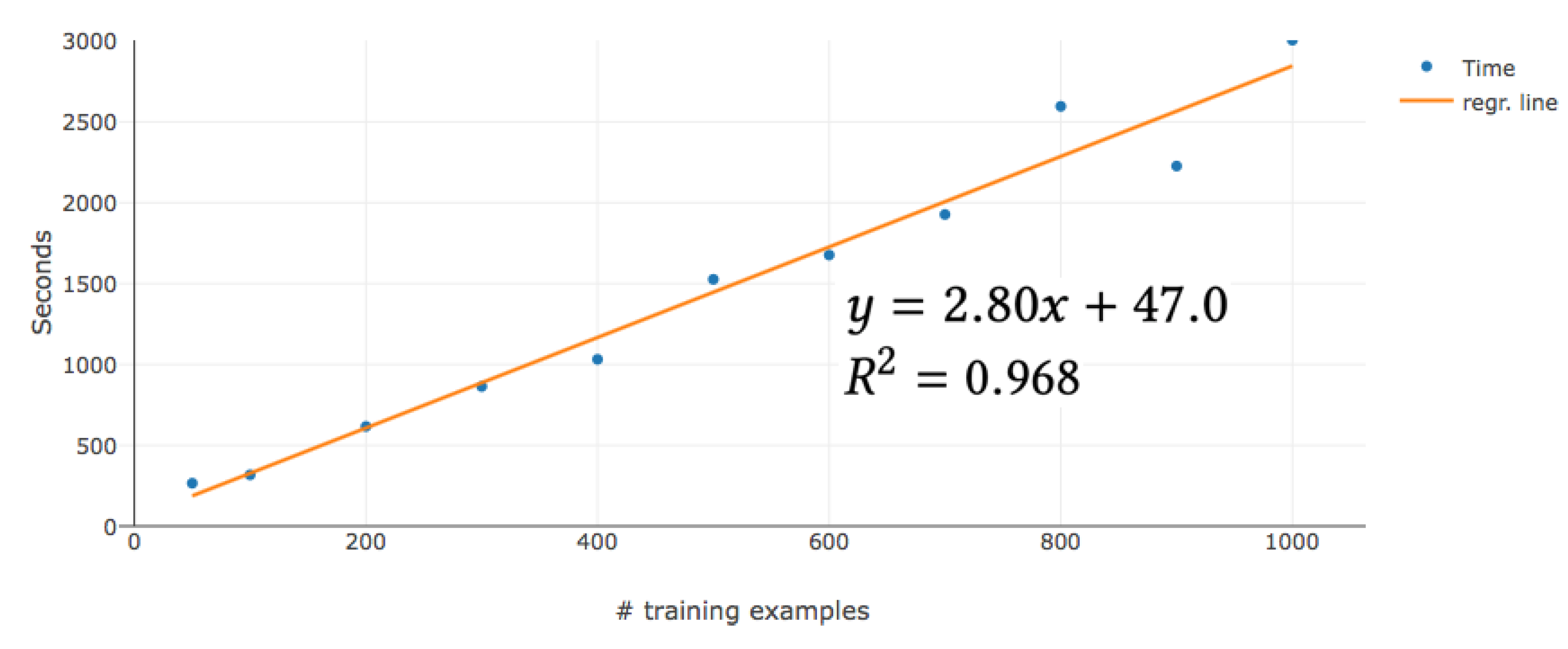
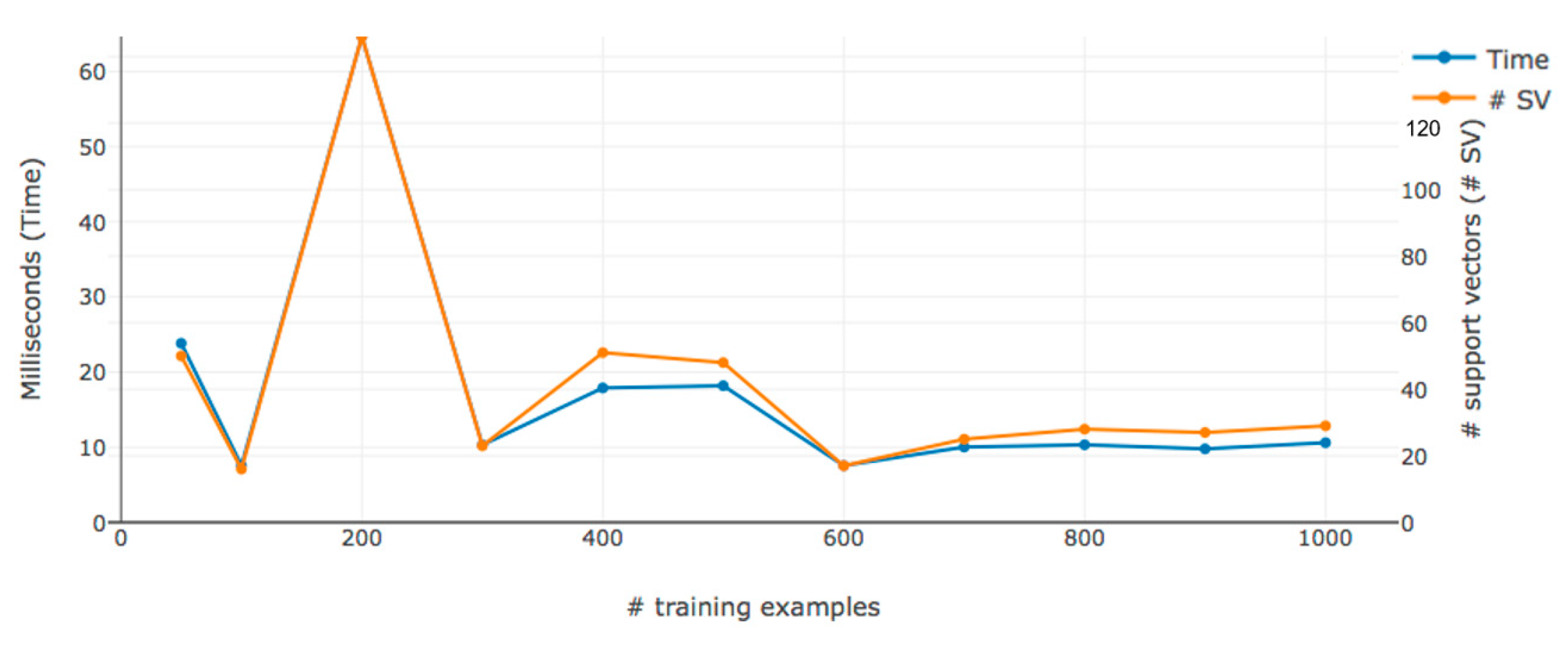
  • Linear time algorithms to compute the subpath kernel are known [4,5]. Since the time complexity of computing other tree kernels is mostly of the quadratic order of the size of input trees, this advantage is significant. In particular, this enables real-time detection of fake large-scale DOM trees with thousands of vertices.
  • The definition of the subpath kernel is invariant no matter whether trees are ordered or unordered. Although DOM trees are derived as ordered trees, adversaries may change the traversal order of vertices without impacting their logical meaning or layout. Thus, we see that the results by the subpath kernel is secure against the attack of changing the traversal order.

4. The Subpath Kernel

In this section, we look into the subpath kernel more closely.

4.1. Efficient Computing of the Subpath Kernel

In [5], a linear-time algorithm to compute the subpath kernel is presented. It takes a least common prefix (LCP) array as an input, and LCP are computed from a suffix array extracted from trees [5].

4.1.1. Extraction of Suffixes

For better efficiency of computation, the first step of suffix array extraction is assignment of unique identifier to HTML tags. In this section, we use the following assignment.
3:html 4:head ... 6:title 7:link 8:body 9:js 10:div ... 13:img ... 17:a ... 21:span 22:form 23:table 24:tbody 25:tr 26:td ... 65:figure ...
A suffix is a sequence of the identifiers of HTML tags of a subpath from a vertex of a DOM tree to the root. Figure 9 exemplifies a DOM tree and all the suffixes extracted from it. Since the DOM tree consists of 17 vertices, 17 suffixes are extracted. For example, a subpath tr:tbody:table:body:html corresponds to a suffix [25,24,23,8,3]. In the suffix array, suffixes are sorted in the lexicographical order. A linear-time algorithm to compute the sorted suffix array is presented in [4].

4.1.2. Generation of Least Common Prefix Arrays

To generate an LCP array for two trees x and y, the suffix arrays of x and y are first merged and are the sorted in a lexicographical order. Table 1 shows an example: suffixes extracted from x of Figure are displayed in red, while y in black.
The LCP length for a suffix in the merged array is determined by the length of the longest common prefix between the suffix and the next suffix. For example, the suffixes of [26,25,10,24,23,8,3] and [26,25,24,23,8,3] are adjacent, and their longest common prefix is [26,25]. Therefore, the LCP length assigned to [26,25,10,24,23,8,3] is two as displayed in red. 1 is assigned to the last suffix.

4.2. Understanding the Decay Factor α

When computing K SP ( x , y ) , a subpath with n vertices shared between x and y is counted by a factor of α n . Therefore, the contribution of long subpaths increases, as α becomes greater. To be precise, if a subpath with n vertices is shared by x and y, they also share i subpaths with n + 1 i vertices, and therefore, its contribution to the kernel value is evaluated by
γ ( n , α ) = i = 1 n i α n + 1 i = α α 1 α n + 1 1 α 1 n 1 , if α 1 ; n ( n + 1 ) 2 , if α = 1 .
Figure 10 shows the change of the ratio γ ( 10 , α ) γ ( m , α ) , when m and α changes. We see that a single subpath with ten vertices is equivalent to 91 subpaths with two vertices for α = 1.5 , and the number rapidly decreases as m increases and α decreases.

5. The Proposed Method

After seeing the entire picture of the steps of our detection system, we see experimental results on the performance of each step. In the experiments, we use iMac Pro with 14 core 2.5 GHz Intel Xeon W and 128 Gbyte memory.

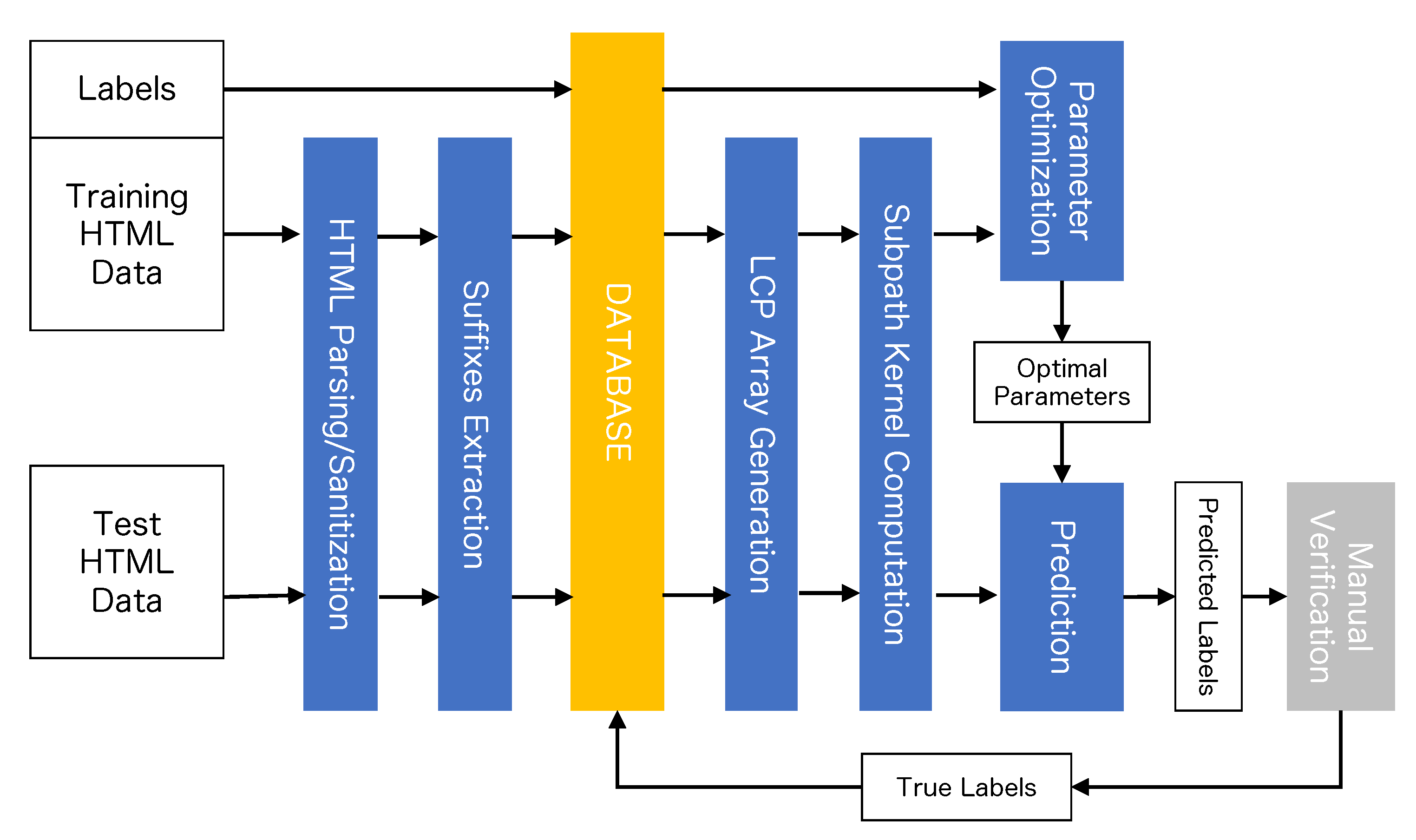
5.1. The Entire Picture

Figure 11 depicts the entire structure of our proposed system. HTML mark-up documents are first input into an HTML parsing/sanitization program, which extract DOM trees from them after eliminating and correcting non-standardized descriptions included. The obtained DOM trees are input into a suffixes extracting program (Section 4.1.1), and the obtained suffix arrays are stored in a database. Since the suffix array of a DOM tree will be used for multiple times to compute the subpath kernel values with other DOM tree, storing the suffix array in a database will be beneficial to improve the efficiency of the entire process.
In the next step, the necessary subpath kernel values are computed. When a training dataset consists of DOM trees x 1 , , x n , the complete Gram matrix
G ( x 1 , x n ) = k ( x 1 , x 1 ) k ( x 1 , x n ) k ( x n , x 1 ) k ( x n , x n ) .
Is computed. k ( x i , x j ) is the normalized value of the subpath kernel value K SP determined by
k ( x i , x j ) = K SP ( x i , x j ) K SP ( x i , x i ) K SP ( x j , x j ) .
The normalization is necessary to eliminate undesirable effects caused by different sizes of DOM trees (Section 3.1). For the prediction purpose, kernel values are computed only between the DOM trees in a test dataset and the DOM trees that comprise support vectors in the training dataset. To compute the subpath kernel value K SP ( x , y ) , the LCP array between x and y is first computed (Section 4.1.2), and then, it is input into the linear-time algorithms presented in [5].
In the step of parameter optimization, the optimal values for the two hyper-parameters of the decay factor α and the regulation coefficient C of SVC are computed through a grid search algorithm.
In the prediction step, a separating hyper-plane in the reproducing kernel Hilbert space is computed with the training dataset and the associated optimal hyper-parameters, and then, a predicted label of a DOM tree in the test dataset is computed by SVC.

5.2. Suffixes Extraction

The suffix array extraction program of our system takes a batch of DOM trees as inputs, and then, computes the associated suffix arrays efficiently through parallel computation. Figure 12 shows the averaged time in milliseconds to extract suffix arrays from a single DOM tree, when changing the batch size from 50 to 1000. Although the time scores for n = 50 and 100 are higher because of the overhead of parallel computation, we see that our program can process a single DOM tree in 20 milliseconds on average.

5.3. Gram Matrix Generation

Since a Gram matrix is symmetric, to compute an n-dimensional Gram matrix, computation of n ( n + 1 ) 2 kernel values is necessary. Hence, the effect of deploying parallel computation is expected to be greater than used for suffix array extraction.
Figure 13 shows the total run-time scores of computing Gram matrices for n that varies from 50 to 1000. Although the total run-time (the blue line) should be in theory proportional to the number of kernel values to compute (the orange line), we can see a gap between them that is caused by the overhead of using parallel computation.
In fact, Figure 14 plots the averaged computation time to compute a single kernel value, that is, the ratio of the total run-time to the number of kernel values. the effect of the overhead is evident, when n is small. As n increases, the contribution of parallel computation becomes remarkable, and the averaged time only as great as 60 microseconds.

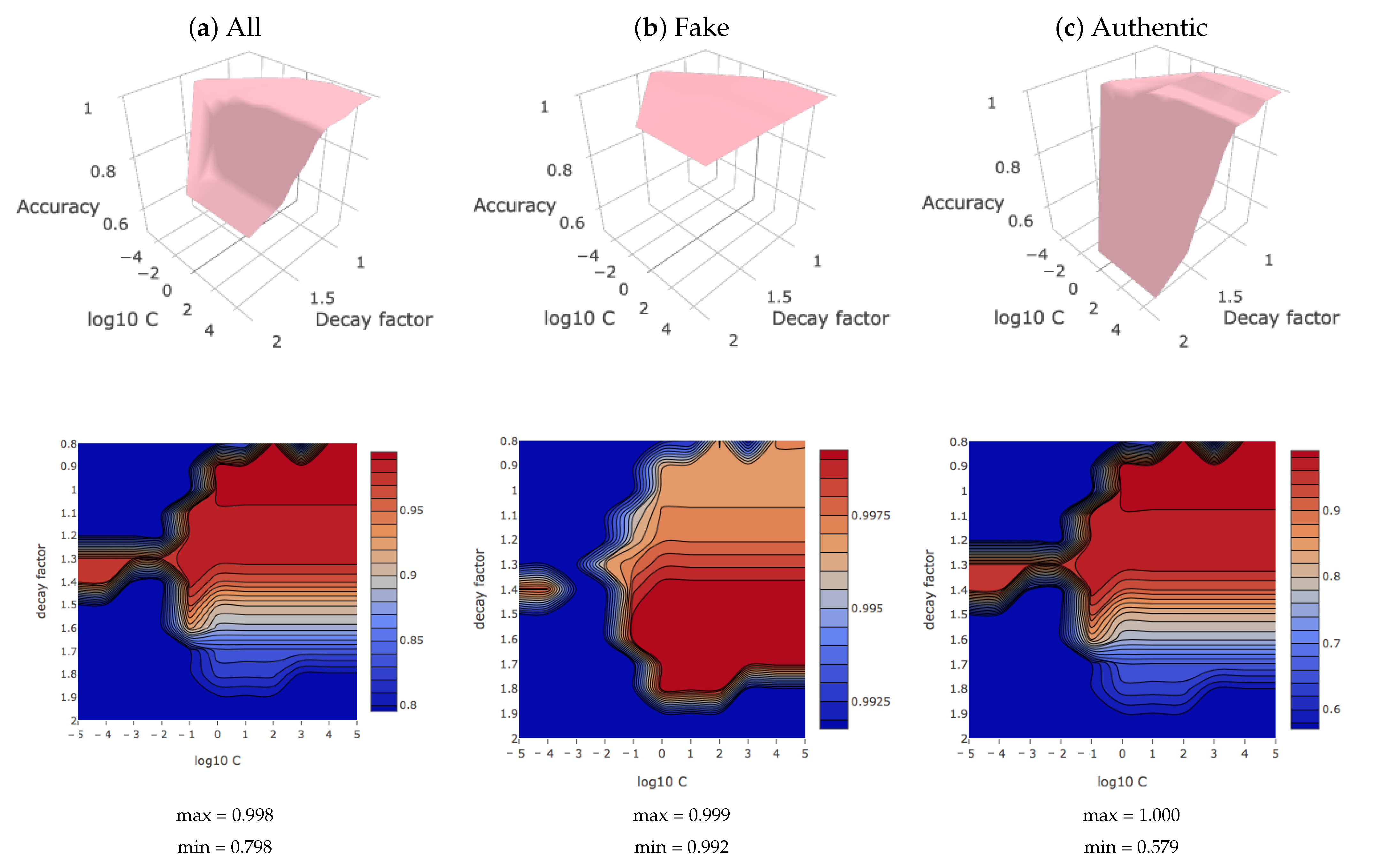
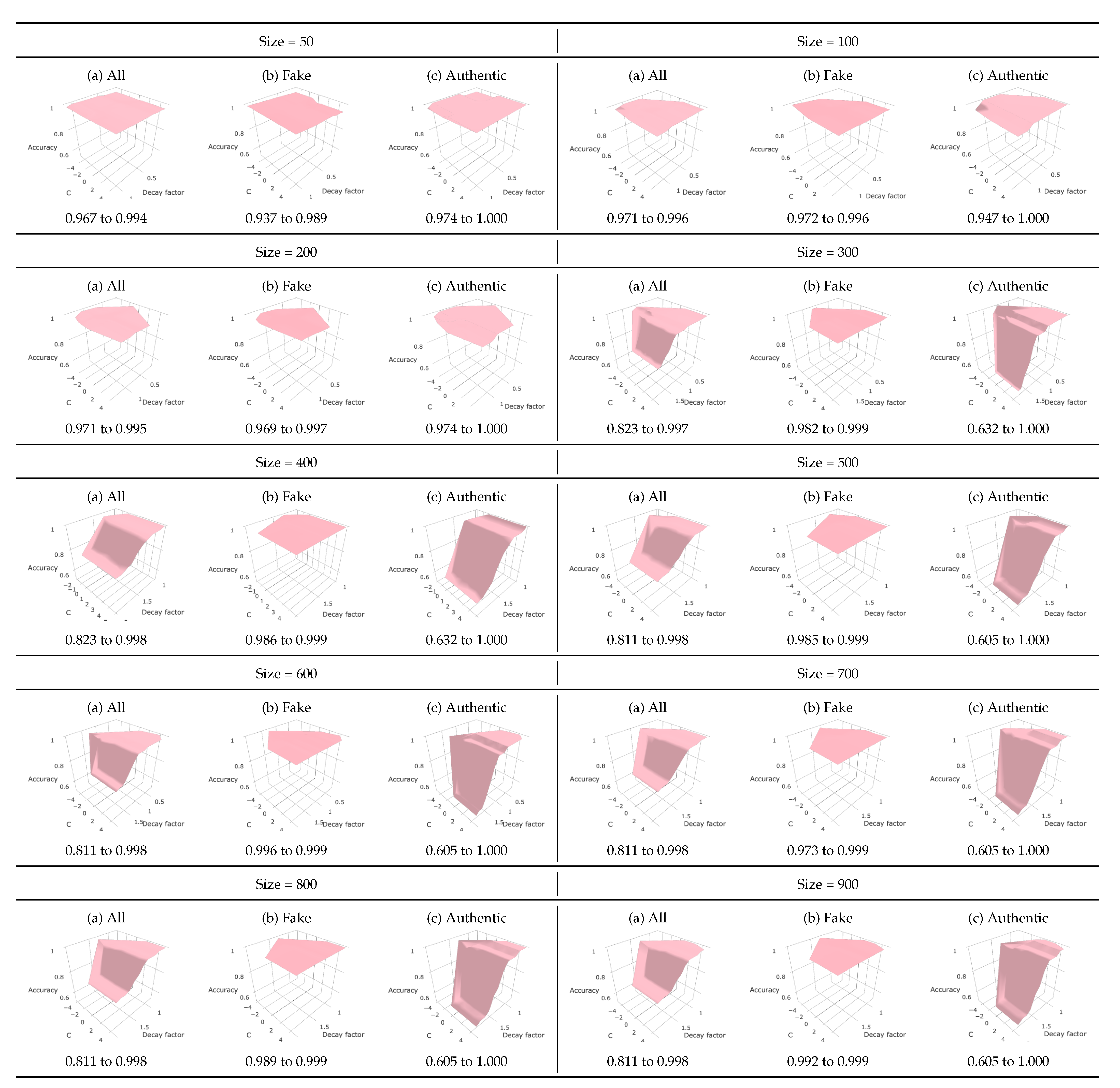
5.4. Hyper-Parameter Optimization

To build optimal models, there are two adjustable hyper-parameters: the decay factor α for the subpath kernel and the regulation coefficient C for SVC. Our program for hyper-parameter optimization performs a simple grid search by changing α from 0.1 to 2.0 with an interval 0.1 and log 10 C from 5 to 5 with an interval 1. The total number of different combinations of α and C to test is 220. For evaluation of each combination of α and C, cross-validation scores with five folds are used. We evaluate the performance of this step from both efficiency and accuracy points of view.
Figure 15 shows that the relationship between the total run-time for optimizing the hyper-parameters and the size n of training datasets can be fit to an increasing regression line with a determination coefficient as high as 0.968. Furthermore, the run-time for n = 1000 is 3004 s ≈ 50 min. Due to the excellent generalization performance of SVC, we can obtain good models even for n 1000 , and hence, model updates can be performed quickly.
Figure 16a consists of a plane view and a contour plot of the cross-validation scores (accuracy scores) obtained through the grid search for n = 1000 . Except that there is a steep drop-off where the score falls from 1.0 to 0.857 within the rectangular area with 1.4 α 12.0 and 5 log 10 C 1 , the score is mostly 1.0.
When investigating the cases of fake and authentic sites separately (Figure 16b,c, the accuracy score for the fake sites, computed by TP TP + FN , varies within a narrow range between 0.976 and 1.0, while the score for the authentic site, computed by TN TN + FP , has a steep drop-off in the same rectangular area as the score for the entire dataset.
For the smaller training datasets we have tested, we observe the same property for most of cases (Figure 17). In particular, the maximum cross-validation is 1.0 for all the cases including when the dataset size is as small as 50.

5.5. Prediction

Next, using the 5946 validation examples, we test only the parameter combinations that have shown the highest cross-validation score of 1.0. Figure 18a shows the obtained accuracy scores. Interestingly, it turns out that the score drops rapidly from 0.98 to 0.8, when the decay factor exceeds 1.3. This implies that overfitting has occurred. When we focus on the fake sites, as Figure 18b shows, the range of the accuracy score is very narrow between 0.999 and 0.992, and the identification problem of fake sites turns out not to be sensitive to hyper-parameter selection. On the other hand, Figure 18c shows that learning of authentic sites with a decay factor higher than 1.3 is likely to generate overfitting models, whose accuracy score can be as low as 0.579.
As seen in Section 4.2, the subpath kernel with a high decay factor evaluates longer shared subpaths more significantly. Hence, the results of the validation shows that pages of authentic sites are better characterized by shorter subpaths rather than longer subpaths.
Furthermore, Figure 19 shows the results of validation when we use training datasets whose size are smaller than 1000. Surprisingly, even small datasets can exhibit very high accuracy, and for example, a dataset with only 50 examples shows the accuracy score of 0.994. Also, we can observe overfitting occurring in the same way and under almost the same conditions as when we use a dataset of size 1000, and SVC shows the best accuracy performance when the parameters are selected from the area of 0.9 α 1.1 and 0 log 10 C 5 .
Once the hyper-parameters α and C are specified, we will be able to make prediction on which unknown sites are fake or authentic based on their DOM trees.
The first step of prediction is the step to train an SVC based on the hyper-parameter values obtained in the previous optimization process and the training dataset used. The output of training SVC is a model that specifies the separating hyperplane computed through training.
In our system, we assume that, once an SVC is trained, we continue to use the same SVC to make many predictions. Hence, the time efficiency of training an SVC is not significantly critical.
Figure 20 shows the runtime t in seconds to train an SVC when the size n of a dataset varies. When excluding one outlier ( n = 400 ), the relation between t and n fits to a line with determination coefficient 0.990 . When n = 400 , the objective function has converged exceptionally slowly, and the program of libSVM [36] has reached the default upper limit of 10,000,000 iterations. Including this exceptional datum, the total runtime for training does not one minute largely. We can conclude that.
The actual output of training an SVC is a subset of examples of a training dataset, which uniquely determines a hyperplane. To make a prediction on a new DOM tree, it suffices to compute the kernel values between the new DOM tree and the support vectors Since these DOM trees have been converted into suffix arrays in the suffix arrays extraction process, computing these kernel values can be performed very quickly by taking advantages of the algorithm introduced by [5].
In fact, Figure 21 shows the averaged runtime to make a prediction for a single unknown DOM tree and the number of support vectors for eleven training datasets with different sizes. We can see that the runtime and the number of support vectors are faithfully proportional. Although the runtime for n = 200 is exceptionally high, it is only 65 milliseconds. For the other datasets the scores are lower than 25 milliseconds. This indicates that our system can sufficiently realize real-time detection of fake sites.

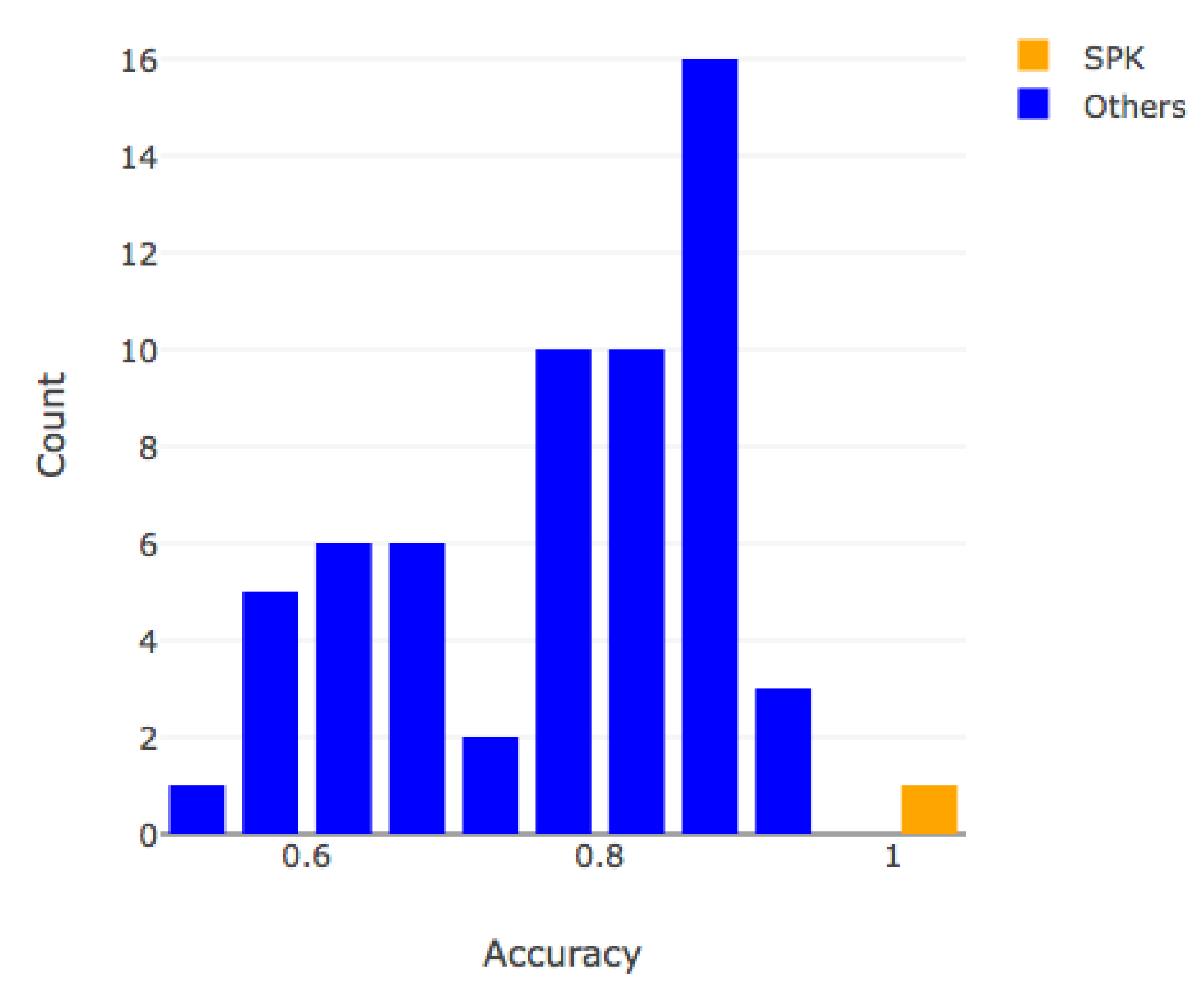
5.6. Comparison in Accuracy Performance

Table 2 exhibits the results of comparison of our method trained by 100 and 1000 data, respectively, against seven benchmark methods for phishing site detection in terms of accuracy performance. The accuracy performance is evaluated using four measures of precision, recall, F-score and accuracy rate, if possible. We see that our method trained with 1000 data (500 fake and 500 authentic) outperforms the others for all of the four measures. Interestingly, even when our method is trained with only 100 data, the measurements are almost compatible with the best of the benchmark methods.
Mainly because the datasets used for the evaluation are different according to the methods, we cannot statistically conclude that our method is superior to the benchmark methods. However, we should emphasize that our method leverages robust features derived from distributions of subpaths in DOM trees. In contrast, the benchmark methods mainly rely on shallow features, which the adversaries can alter without difficulties.
Furthermore, we should note the fact that our method exhibited high accuracy performance using small datasets for training and significantly larger datasets for testing. This observation should be a clear evidence that indicates the excellent generalization performance of our method. The practical meanings of this observation are: we can reduce the frequency of model renewal; and the model renewal by itself can be performed significantly efficiently.

6. Conclusions

We have shown a method to realize highly accurate and real-time detection of fake e-commerce sites based on DOM tree similarity. We demonstrated its accuracy and speed on a real dataset provided by Rakuten. While the efficiency and performance of our method alone make it compelling, another advantage is the minimal amount of training data required. We believe our method has the potential to increase the safety of e-commerce solutions. Not only does it detect fake sites quickly and with high accuracy, given that it requires only small training data sets, it allows web security software to update itself more quickly against new threats as they emerge.

Author Contributions

K.S. developed the core idea of applying the subpath kernel to fake website detection; K.S. and T.I. contributed equally to prototyping, performing experiments, writing text and generating graphics; Y.-L.L. prepared the datasets used in the experiments and gave technical advice as an information security expert; D.L.S. offered guidance as an expert in machine learning and contributed to the writing process. All authors have read and agreed to the published version of the manuscript.

Funding

This work was partially supported by the Grant-in-Aid for Scientific Research (JSPS KAKENHI Grant Number 17H00762) from the Japan Society for the Promotion of Science.

Institutional Review Board Statement

Not applicable.

Informed Consent Statement

Not applicable.

Data Availability Statement

Data sharing not applicable (The original fake e-commerce sites are no longer available because, as a result of this research, most were shut down).

Acknowledgments

The authors received valuable information on cyber crimes committed relating to fake e-commerce sites from Hyogo Prefectural Police.

Conflicts of Interest

The authors declare no conflict of interest.

Appendix A. A Theory of Positive Definite Kernels

A real-valued kernel is a symmetric bivariable function K : X × X R defined over a set X . A positive definite kernel, on the other hand, is defined by
Definition A1.
A kernel K : X × X R is positive definite, if, and only if, i = 1 n j = 1 n c i c j K ( x i , x j ) 0 holds for any n N , { x 1 , , x n } X and { c 1 , , c n } R .
The simplest example of positive definite kernels is a dot product over a finite dimensional vector space X = R n : the dot product of v = ( v 1 , , v n ) and w = ( w 1 , , w n ) in R n is determined by v · w = i = 1 n v i w i . In reverse, Theorem A1 asserts that any positive definite kernel can be viewed as an inner product defined over a linear space.
An n-dimensional matrix [ K ( x i , x j ) ] i , j = 1 , , n given for { x 1 , , x n } X is referred to as a Gramian matrix, and K is positive definite, if, and only if, the Gramian matrix for any { x 1 , , x n } X has no negative eigenvalues [28]. For a positive definite kernel, we have
Theorem A1.
(Schönberg [28]). K is positive definite, if, and only if, there exists a projection π of X into a real Hilbert space H with inner product · , · such that K ( x , y ) = π ( x ) , π ( y ) for any ( x , y ) X × X . This H is called the reproducing kernel Hilbert space (RKHS).
A Hilbert space H is a linear space with inner product such that any Cauchy series with respect to the topology induced from the inner product converges to a point in H . The dimension of the RKHS of finite X is bounded above by | X | .
When X R D , positive definite kernels is commonly used to obtain linear separability, an important condition to apply some classifiers such as the support vector classifier (SVC). If a hyperplane separates sets of positive examples P = { v 1 , , v m } and negative examples N = { w 1 , , w n } , we say that P and N are linearly separable. For P and N that are not linearly separable, we can leverage Theorem A1 to map the points of X in a Hilbert space H so that the images of P and N become linearly separable in H . For this purpose, we can use Gaussian kernels, also known as RBF kernels, defined by G ( x , y ) = exp x y 2 2 σ 2 , for example.
Theorem A1 proves its merits, when the elements of X are not vectors. In fact, we assume that X is a space of (DOM) trees in this paper. The projection π maps trees to points in H , and hence, we become capable to apply multivariate analysis to the projected points. Moreover, many techniques of multivariate analysis rely only inner products of the projected points, and their inner products can be computed through the kernel function. This proves to be significantly faster in many cases than direct computation of inner products in H , which can be highly dimensional.
To obtain positive definite kernels for trees, the convolution kernel and Haussler’s theorem are a fundamental tool. We assume a kernel k : Ω × Ω R defined over a set Ω and let X consist of finite subsets of Ω . For ( x , y ) X × X ,
K ( x , y ) = ( v , w ) x × y k ( v , w )
Defines a convolution kernel. In our setting, Ω is a space of vertices, and k is a similarity function for vertices. A typical example of k is Kronecker’s delta function δ v , w on labels of vertices: if two vertices v and w have the same label, k ( v , w ) = 1 , and k ( v , w ) = 0 , otherwise. Moreover, we denote a tree with a vertex set x Ω by the same symbol x, and therefore, the associated convolution kernel is a tree kernel.
Haussler’s theorem asserts.
Theorem A2.
(Haussler [29]). If k is positive definite, the associated convolution kernel K is positive definite.

Appendix B. Rooted Ordered Trees

We first define rooted trees. In this paper, we define a rooted tree as a particular class of partially ordered sets.
We let ( V , ) be a partially ordered set. Hence, the following hold: v v ; v = w if v w and w v ; v u if v w and w u . We denote v < w , if  v w and v w .
Definition A2.
A partially ordered set ( V , ) is a rooted tree, if, and only if, the following conditions are met.
  • The root r V exists such that r v for any v V .
  • For any v V , V v = { w w v } is totally ordered.
In the definition, V means a set of vertices of a tree, and the order ≤ determine a generation order. We say v V is an ancestor of w V , if v < w holds. If v is the nearest ancestor of w, we denote v w and say that v is the parent of w and w is a child of v. A vertex with no children is called a leaf. Also, the nearest common ancestor v w is defined for { v , w } V by
Definition A3.
The nearest common ancestor v w is the maximum vertex of V v , w = { u V u v , u w } .
For any ( v , w ) V × V , v w always exists and is unique.
On the other hand, a rooted tree t with an entire set of leaves L is called an ordered tree, when
Definition A4.
If the leaves is numbered by L = { l 1 , , l | L | so that l i l j l k = l i l k holds for any 1 i < j < k L , we say that the tree is ordered.
Figure A1 exemplifies a numbering of leaves of an ordered tree. Also, a leaf numbering canonically introduces a traversal order among vertices.
Figure A1. An ordered tree.
Make 03 00006 g0a1
Definition A5.
For two distinct vertices v and w of a rooted ordered tree ( V , ) , we define v w , if, and only if, max { i l i v } < min { i l i w } holds.
In Figure A1, head body follows max { i l i head } = 2 < 3 = min { i l i body } .

Appendix C. Edit Distances for Trees

We briefly study edit distances for trees. In particular, we introduce the constrained distance (Appendix C.3) and the degree-two distance (Appendix C.4).

Appendix C.1. Taï Distance and Its Variations

Levenshtein [2] first defined the first instance for strings, and later, Taï [1] extended it to trees. The Taï distance is defined as the minimum length of paths from a tree t 1 to another tree t 2 in the entire graph of trees. The graph includes trees as vertices, while an edge is defined between a tree and another, if, and only if, one is converted into the other by substitution, deletion or insertion of a single vertex. For example, Figure A2 depicts the shortest path t 1 t 2 t 3 t 4 , and hence, the Taï distance of t 1 and t 2 is 3. Many efforts to improve the Taï edit distance in particular in terms of computational efficiency followed, and we have many variations [39,40,41,42,43,44,45,46,47] (See Appendix C),
Figure A2. Taï distance between t 1 and t 4 is three.
Make 03 00006 g0a2
Taï distance is not only the first tree edit distance proposed in the literature but also the most common. An important problem Taï distance is its high computational complexity. Computing Taï distances for unordered rooted trees is known NP-hard. Although its computational complexity for ordered rooted trees is polynomial-time, the original algorithm presented in [1] required significantly heavy computation in practice.
Much effort has been made to develop efficient algorithms to compute Taï distances.
  • Zhang and Shasha [40] proposed an algorithm of
    O ( | X | | Y | min ( w ( X ) , h ( X ) ) min ( w ( Y ) , h ( Y ) ) ) -time: X and Y denote rooted ordered trees; | X | , w ( X ) and h ( X ) denote the size (the number of vertices), the width (the number of leaves) and the height (the length of the longest path from the root to a leaf) of X. According to shapes of trees, this varies between O ( | X | | Y | ) and O ( | X | 2 | Y | 2 ) .
  • Klein [48] improved the efficiency to O ( | X | 2 | Y | log | y | ) -time by taking advantage of decomposition strategies [49].
  • Demaine et al. [50] further optimized this technique and presented an algorithm of O ( | X | 3 ) -time. Demaine’s algorithm is the fastest in terms of the asymptotic evaluations, but it easily lapses into the worst case. Therefore, the algorithm of Zhang and Shasha in fact outperforms Demaine’s algorithm in many practical cases.
  • RTED, an algorithm that Pawlik and Augsten [51] have developed, not only has the same asymptotic complexity as Demaine’s algorithm but also almost always outperforms the competitors in practice.
Furthermore, the space complexity of Zhang’s algorithm, Demaine’s algorithm and RTED is O ( | X | | Y | ) , which is practically small.
Although the aforementioned improvement in efficiency was remarkable, the asymptotic time complexity of O ( | X | 3 ) is still too heavy for some practical applications. In the literature, several new distances have been proposed to take over Taï distance. In the following, we introduce two of the most important examples of them.

Appendix C.2. Mappings Associated with Edit Paths

In Section 3.1, we have introduced a graph of trees so that the vertices of the graph are trees, while an edge connecting two trees X and Y means that X is converted into Y by a single edit operation, which is one of substituting a new label for the label of a vertex of X, deleting a vertex of X and inserting a vertex of Y (Figure A2). An edit path, on the other hand, is a path in the graph, and therefore, represents a sequence of edit operations that converts the source tree into the destination tree.
An edit path from X to Y associates a vertex v of X which the edit path does not delete with a vertex μ ( v ) of Y with which the edit path replaces the v. The entire collection of such ( v , μ ( v ) ) determines a mapping, that is, a subset μ X × Y . For simplicity, we let the same symbols of X and Y denote the vertex sets of the trees X and Y. We call this μ the mapping associated with the edit path. A mapping associated with an edit path is one-to-one. Furthermore, Taï proved
Theorem A3.
(Ref. [1]). For rooted ordered trees X and Y, a mapping μ X × Y is associated with some edit path, if, and only if, μ preserves the generation and traversal orders of X and Y.
This theorem also asserts that M X , Y T is identical to the set of mappings associated with edit paths. With M X , Y T , Taï distance is determined by
d T ( X , Y ) = | X | + | Y | ( v , w ) M X , Y T ( δ v , w + 1 ) .
The function δ v , w is 1, if the labels of v and w are identical, and 0, otherwise.

Appendix C.3. The Constrained Distance

The constrained distance [52] is defined by imposing the certain constraint described below on mappings of Taï distance. Zhang has also presented an efficient algorithm to compute constrained distances, whose time and space complexity is O ( | X | | Y | ) . Although Richter [53] independently introduced the structure-respecting distance tailoring Taï distance to particular applications, Bille [54] has shown the identity between the constrained and structure-respecting distances.
To describe the constraint of the constrained distance, we have to introduce the concept of separable vertex sets.
Definition A6.
We let S and T be two subsets of vertices of a tree and let S ( T ) denote the nearest common ancestors of the vertices in S (T). S and T are separable, if, and only if, neither S T nor S T holds.
Definition A7.
A mapping μ X × Y is said to be separable, if, and only if, (1) μ preserves the generation and traversal orders of X and Y and (2) μ ( S ) and μ ( T ) are separable in Y for any separable subsets S and T in in X.
The partial mapping depicted by Figure A3 is separable.
Definition A8.
An edit path of Taï distance is said to be separable, if, and only if, the associated mapping is separable.
We denote the entire set of separable edit paths from X to Y by Π X , Y S and the entire set of mappings associated with edit paths in Π X , Y S by M X , Y S . Then, the constraint distance d C ( X , Y ) is determined by
d C ( X , Y ) = min π Π X , Y S | π | = | X | + | Y | ( v , w ) M X , Y S ( δ v , w + 1 ) .
Figure A3. A separable mapping { ( v i , w i ) } i = 1 , 1 , 5 M x , y S .
Make 03 00006 g0a3

Appendix C.4. The Degree-Two Distance

The degree-two distance [41] imposes the following constraint on the primitive edit operations of deletion and insertion: roots must not be deleted or inserted; only vertices with degree one and two can be deleted and inserted. The degree of a vertex is the number of edges that the vertex has, and the degree-two distance is the minimum length of edit paths under this constraint. The time and space complexity of the degree-two distance is O ( | X | | Y | ) .
Figure A4 exemplifies an edit path of the degree-two distance. In X, the vertex v d is of degree one, and hence, we can delete it under the constraint of the degree-two distance. By deleting v d , the degree of v b has changed from three to two in X 2 , and hence, we are allowed to delete it. Also, we can insert v f between v a and v g , because the resulting degree of v f in X 5 is two. For the same reason, we can insert v d below v f . The length of this edit path is five. Also, it is easy to see that the shortest edit path under the constraints, and hence the degree-two distance between X and Y turns out to be five. We have
Theorem A4.
For μ X × Y that preserves the generation and traversal orders, μ be a mapping associated with an edit path of the degree-two distance, if, and only if, ( v v , w w ) μ holds for any ( v , w ) μ and ( v , w ) μ .
Thus, we see that M x , y E is identical to the entire set of mapping associated with edit paths of the degree-two distance. Hence, the degree-two distance d D 2 ( X , Y ) between X and Y is determined by
d D 2 ( X , Y ) = | X | + | Y | ( v , w ) M X , Y E ( δ v , w + 1 ) .
Figure A4. An edit path of the degree-two distance.
Make 03 00006 g0a4

Appendix A. Divergences

When we let p and q denote two probability (density) distributions, Kullback-Leibler divergence defined by K L ( p q ) = p ( x ) log q ( x ) p ( x ) d x is the best known example. Since K L ( p q ) = K L ( q p ) does not always hold, we may use Jensen-Shannon divergence 1 2 · K L ( p ( p + q ) / 2 ) + 1 2 · K L ( q ( p + q ) / 2 ) and K L ( p q ) + K L ( q p ) alternatively. Other examples include Bhattacharrya distance ln B H ( p q ) and Hellinger distance 1 B H ( p q ) with Bhattacharyya coefficient B H ( p q ) = ( p ( x ) q ( x ) d x , and L o -norm | p ( x ) q ( y ) | p d x p and Brownian distance 1 min { p ( x ) , q ( x ) } d x .

Appendix E. Positive Definite Kernels and RKHS

Appendix E.1. Properties of of Positive Definite Kernels

We let K : X × X R be positive definite. By Theorem A1, K ( x , y ) is identical to a inner product π ( x ) , π ( y ) in a reproducing kernel Hilbert space H . π : X H is an embedding. Hence, the properties stated below follow from properties of inner products.
Proposition A1.
For positive definite K : X × X R , the following hold.
  • K ( x , x ) 0 .
  • If K ( x , x ) = 0 , then K ( x , y ) = 0 for any y
  • | K ( x , y ) | K ( x , x ) K ( x , y ) . This inequality is known as the Cauchy-Schwartz inequality.
  • d ( x , y ) = K ( x , x ) + K ( y , y ) 2 K ( x , y ) determines a distance over X . This property is follows from the cosine formula.
The following algebraic operations for positive definite kernels preserve positive definiteness.
Proposition A2.
We let K and K i : X × X R be positive definite for i = 1 and 2. Then, we have
  • For a 0 and b 0 , the linear combination a K 1 + b K 2 is positive definite.
  • The product K 1 · K 2 is positive definite.
  • For any non-negative integer n 0 , the power K n is positive definite.
  • For any polynomial f ( X ) R [ X ] with only positive coefficients, f ( K ) is positive definite.
Even if a real number r R is positive, K r is not necessarily positive definite. If K r is always positive definite for r > 0 , K is said to be infinitely divisible.
If K ( x , x ) = 0 , x is trivial in the sense that it is projected to the zero vector in RKHS. Thus, we eliminate all x with K ( x , x ) = 0 from X and assume that K ( x , x ) > 0 for any x. Then, we can define the normalized kernel of K by
K N ( x , y ) = K ( x , y ) K ( x , x ) K ( y , y ) .
Proposition A3.
We let K : X × X R be a kernel with K ( x , x ) > 0 . K is positive definite, if, and only if, its normalization K N is positive definite.
This property follows from Lemma A1 and Proposition A2.
Lemma A1.
For arbitrary function f : X R , K ( x , y ) = f ( x ) f ( y ) determines a positive definite kernel.

Appendix B.2. RKHS for Finite Sets

If X is a finite set, the associated reproducing kernel Hilbert space H turns out to be a finitely dimensional inner product space. Furthermore, we can explicitly constitute the projection mapping π : X R | X | with the property of K ( x , y ) = π ( x ) T π ( y ) . This can be proven easily as follows.
We let G be the Gramian matrix induced from a positive definite K and a finite set X = { x 1 , , x n } :
G = K ( x 1 , x 1 ) K ( x 1 , x n ) K ( x n , x 1 ) K ( x n , x n ) .
By Schure decomposition, G = U T A U holds for some orthogonal matrix U R n × n and some upper triangular matrix A R n × n . G is normal ( G G T = G T G ), and hence, A turns out to be normal as well. Since a normal triangular matrix is always diagonal, A is a diagonal matrix and its diagonal elements constitute the eigenvalues of G. In particular, all of the diagonal elements of A are non-negative, since G is positive (semi-)definite, and a diagonal matrix A such that A A = A can be determined. Hence, we have
G = ( A U ) T ( A U ) .
We let A U = [ v 1 , , v n ] with column vectors v i R n and define π by π ( x i ) = v i . K ( x i , x j ) = v i T v j holds.

References

  1. Taï, K.C. The tree-to-tree correction problem. J. ACM 1979, 26, 422–433. [Google Scholar] [CrossRef]
  2. Levenshtein, V.I. Binary codes capable of correcting deletions, insertions, and reversals. Sov. Phys. Dokl. 1966, 10, 707–710. [Google Scholar]
  3. Collins, M.; Duffy, N. Convolution Kernels for Natural Language. In Advances in Neural Information Processing Systems 14 [Neural Information Processing Systems: Natural and Synthetic, NIPS 2001]; MIT Press: Cambridge, MA, USA, 2001; pp. 625–632. [Google Scholar]
  4. Kimura, D.; Kashima, H. Fast Computation of Subpath Kernel for Trees. arXiv 2012, arXiv:1206.4642. [Google Scholar]
  5. Shin, K.; Ishikawa, T. Linear-time algorithms for the subpath kernel. In Proceedings of the 29th Annual Symposium on Combinatorial Pattern Matching (CPM 2018), Qingdao, China, 2–4 July 2018; pp. 22:1–22:13. [Google Scholar]
  6. Corona, I.; Biggio, B.; Contini, M.; Piras, L.; Corda, R.; Mereu, M.; Mureddu, G.; Ariu, D.; Roli, F. DeltaPhish: Detecting Phishing Webpages in Compromised Websites. arXiv 2017, arXiv:1707.00317. Available online: https://arxiv.org/abs/1707.00317 (accessed on 13 January 2021).
  7. Zhang, Y.; Egelman, S.; Cranor, L.; Hong, J. Phinding Phish: Evaluating anti-phishing tools. In Proceedings of the 14th Anual Network and Distributed System Security Symposium, San Diego, CA, USA, 28 February–2 March 2007. [Google Scholar]
  8. Li, L.; Helenius, M. Usability Evaluation of Anti-Phishing Toolbars. J. Comput. Virol. 2007, 3, 163–184. [Google Scholar] [CrossRef]
  9. Abbasi, A.; Chen, H. A comparison of tools for detecting fake websites. Computer 2009, 42, 78–86. [Google Scholar] [CrossRef]
  10. Marchal, S.; Asokan, N. On Designing and Evaluating Phishing Webpage Detection Techniques for the Real World. In Proceedings of the 11th USENIX Workshop on Cyber Security Experimentation and Test (CSET 18), Baltimore, MD, USA, 11–13 August 2018; USENIX Association: Baltimore, MD, USA, 2018. [Google Scholar]
  11. Corona, I.; Biggio, B.; Contini, M.; Piras, L.; Corda, R.; Mereu, M.; Mureddu, G.; Ariu, D.; Roli, F. DeltaPhish: Detecting Phishing Webpages in Compromised Websites. Lect. Notes Comput. Sci. 2017, 10492, 370–388. [Google Scholar]
  12. Liu, W. An antiphishing strategy based on visual similarity assessment. IEEE Internet Comput. 2006, 10, 58–65. [Google Scholar]
  13. Satish, S.; Babu, K.S. Phishing Websites Detection Based on Web Source Code and URL in the Webpage. Int. J. Comput. Sci. Eng. Commun. 2013, 1, 1–5. [Google Scholar]
  14. Marchal, S.; Saari, K.; Singh, N.; Asokan, N. Know Your Phish: Novel Techniques for Detecting Phishing Sites and Their Targets. In Proceedings of the 2016 IEEE 36th International Conference on Distributed Computing Systems (ICDCS), Nara, Japan, 27–30 June 2016; pp. 323–333. [Google Scholar]
  15. Whittaker, C.; Ryner, B.; Nazif, M. Large-Scale Automatic Classification of Phishing Pages. In Proceedings of the NDSS ’10, San Diego, CA, USA, 28 February–3 March 2010. [Google Scholar]
  16. Zhang, Y.; Hong, J.I.; Cranor, L.F. Cantina: A Content-based Approach to Detecting Phishing Web Sites. In Proceedings of the 16th International Conference on World Wide Web, Banff, AB, Canada, 8–12 May 2007; ACM: New York, NY, USA, 2007; pp. 639–648. [Google Scholar] [CrossRef]
  17. Marchal, S.; François, J.; State, R.; Engel, T. PhishStorm: Detecting Phishing With Streaming Analytics. IEEE Trans. Netw. Serv. Manag. 2014, 11, 458–471. [Google Scholar] [CrossRef] [Green Version]
  18. Gerbet, T.; Kumar, A.; Lauradoux, C. (Un)Safe Browsing; Technical Report RR-8594; INRIA: Talence, France, 2014. [Google Scholar]
  19. Raut, P.; Vengurlekar, H.; Shete, R. A Survey of Phishing Website Detection Systems. Int. Res. J. Eng. Technol. 2020, 7, 1145–1148. [Google Scholar]
  20. Vazhayil, A.; Vinayakumar, R.; Soman, K.P. Comparative Study of the Detection of Malicious URLs Using Shallow and Deep Networks. In Proceedings of the 9th International Conference on Computing, Communication and Networking Technologies (ICCCNT), Bengaluru, India, 10–12 July 2018; pp. 1–6. [Google Scholar] [CrossRef]
  21. Yang, P.; Zhao, G.; Zeng, P. Phishing Website Detection Based on Multidimensional Features Driven by Deep Learning. IEEE Access 2019, 7, 15196–15209. [Google Scholar] [CrossRef]
  22. Shima, K.; Miyamoto, D.; Abe, H.; Ishihara, T.; Okada, K.; Sekiya, Y.; Asai, H.; Doi§, Y. Classification of URL bitstreams using bag of bytes. In Proceedings of the 21st Conference on Innovation in Clouds, Internet and Networks and Workshops (ICIN), Paris, France, 19–22 February 2018; pp. 1–5. [Google Scholar] [CrossRef]
  23. Sönmez, Y.; Tuncer, T.; Gökal, H.; Avcı, E. Phishing web sites features classification based on extreme learning machine. In Proceedings of the 2018 6th International Symposium on Digital Forensic and Security (ISDFS), Antalya, Turkey, 22–25 March 2018; pp. 1–5. [Google Scholar] [CrossRef]
  24. Machado, L.; Gadge, J. Phishing Sites Detection Based on C4.5 Decision Tree Algorithm. In Proceedings of the 2017 International Conference on Computing, Communication, Control and Automation (ICCUBEA), Maharashtra, India, 17–18 August 2017; pp. 1–5. [Google Scholar] [CrossRef]
  25. Abbasi, A.; Zhang, Z.; Zimbra, D.; Chen, H.; Nunamaker, J.F. Detecting Fake Websites: The Contribution of Statistical Learning Theory. MIS Q. 2010, 34, 435–461. [Google Scholar] [CrossRef] [Green Version]
  26. Zahedi, F.M.; Abbasi, A.; Chen, Y. Fake-Website Detection Tools: Identifying Elements that Promote Individuals’ Use and Enhance Their Performance. J. Assoc. Inf. Syst. 2015, 16, 2. [Google Scholar] [CrossRef]
  27. Shin, K.; Niiyama, T. The mapping distance—A generalization of the edit distance—And its application to trees. In Proceedings of the 10th International Conference on Agent and Artificial Intelligence, ICAART 2018, Madeira, Portugal, 16–18 January 2018; Volume 2, pp. 266–275. [Google Scholar]
  28. Berg, C.; Christensen, J.P.R.; Ressel, R. Harmonic Analysis on Semigroups. Theory of Positive Definite and Related Functions; Springer: Berlin/Heidelberg, Germany, 1984. [Google Scholar]
  29. Haussler, D. Convolution Kernels on Discrete Structures; UCSC-CRL 99-10; Dept. of Computer Science, University of California at Santa Cruz: Santa Cruz, CA, USA, 1999. [Google Scholar]
  30. Shin, K.; Kuboyama, T. A generalization of Haussler’s convolution kernel—Mapping kernel. In Proceedings of the ICML 2008, Helsinki, Finland, 5–9 June 2008. [Google Scholar]
  31. Shin, K.; Kuboyama, T. A Comprehensive Study of Tree Kernels. In JSAI-isAI Post-Workshop Proceedings; Lecture Notes in Articial Intelligence 8417; Springer: Berlin/Heidelberg, Germany, 2014; pp. 329–343. [Google Scholar]
  32. Kashima, H.; Koyanagi, T. Kernels for Semi-Structured Data. In Proceedings of the 9th International Conference on Machine Learning (ICML 2002), Sydney, Australia, 8–12 July 2002; pp. 291–298. [Google Scholar]
  33. Shin, K. A Theory of Subtree Matching and Tree Kernels based on the Edit Distance Concept. Ann. Math. Artif. Intell. 2015. [Google Scholar] [CrossRef]
  34. Hommel, G. A stagewise rejective multiple test procedure based on a modified Bonferroni tests. Biometrika 1988, 75, 383–386. [Google Scholar] [CrossRef]
  35. Demšar, J. Statistical comparisons of classifiers over multiple data sets. J. Mach. Learn. Theory 2006, 7, 1–30. [Google Scholar]
  36. Chang, C.C.; Lin, C.J. LIBSVM: A Library for Support Vector Machines. 2001. Available online: https://www.csie.ntu.edu.tw/~cjlin/libsvm/ (accessed on 12 January 2021).
  37. Rao, R.S.; Ali, S.T. PhishShield: A Desktop Application to Detect Phishing Webpages through Heuristic Approach. Procedia Comput. Sci. 2015, 54, 147–156. [Google Scholar] [CrossRef] [Green Version]
  38. Tyagi, I.; Shad, J.; Sharma, S.; Gaur, S.; Kaur, G. A Novel Machine Learning Approach to Detect Phishing Websites. In Proceedings of the 2018 5th International Conference on Signal Processing and Integrated Networks (SPIN), Noida, India, 22–23 February 2018; pp. 425–430. [Google Scholar] [CrossRef]
  39. Jiang, T.; Wang, L.; Zhang, K. Alignment of trees—An alternative to tree edit. Theor. Comput. Sci. 1995, 143, 137–148. [Google Scholar] [CrossRef]
  40. Zhang, K.; Shasha, D. Simple Fast Algorithms for the Editing Distance Between Trees and Related Problems. SICOMP 1989, 18, 1245–1262. [Google Scholar] [CrossRef]
  41. Zhang, K.; Wang, J.T.L.; Shasha, D. On the editing distance between undirected acyclic graphs. Int. J. Found. Comput. Sci. 1996, 7, 43–58. [Google Scholar] [CrossRef]
  42. Zhang, K.; Statman, R.; Shasha, D. On the editing distance between unordered labeled trees. Inf. Process. Lett. 1996, 42, 133–139. [Google Scholar] [CrossRef]
  43. Zhang, K. A Constrained Edit Distance Between Unordered Labeled Trees. Algorithmica 1996, 15, 205–222. [Google Scholar] [CrossRef]
  44. Lu, C.L.; Su, Z.Y.; Tang, G.Y. A New Measure of Edit Distance between Labeled Trees. In Lecture Notes in Computer Science; Springer: Berlin/Heidelberg, Germany, 2001; Volume 2108, pp. 338–348. [Google Scholar]
  45. Wang, J.T.L.; Zhang, K. Finding similar consensus between trees: An algorithm and a distance hierarchy. Pattern Recognit. 2001, 34, 127–137. [Google Scholar] [CrossRef]
  46. Kuboyama, T.; Shin, K.; Miyahara, T.; Yasuda, H. A theoretical analysis of alignment and edit problems for trees. In Proceedings of the Theoretical Computer Science, The 9th Italian Conference, Siena, Italy, 12–14 October 2005; pp. 323–337. [Google Scholar]
  47. Neuhaus, M.; Bunke, H. Bridging the Gap between Graph Edit Distance and Kernel Machines; World Scientific: Singapore, 2007. [Google Scholar]
  48. Klein, P.N. Computing the edit-distance between unrooted ordered trees. LNCS 1998, 1461, 91–102. [Google Scholar]
  49. Dulucq, S.; Touzet, H. Analysis of tree edit distance algorithms. In Proceedings of the 14th Annual Symposium on Combinatorial Pattern Matching (CPM), Michoacan, Mexico, 25–27 June 2003; pp. 83–95. [Google Scholar]
  50. Demaine, E.D.; Mozes, S.; Rossman, B.; Weimann, O. An Optimal Decomposition Algorithm for Tree Edit Distance. ACM Trans. Algo. 2006, 6, 2. [Google Scholar]
  51. Pawlik, M.; Augsten, N. RTED: A Robust Algorithm for the Tree Edit Distance. VLDB Endow. 2011, 5, 334–345. [Google Scholar] [CrossRef]
  52. Zhang, K. Algorithms for the constrained editing distance between ordered labeled trees and related problems. Pattern Recognit. 1995, 28, 463–474. [Google Scholar] [CrossRef]
  53. Richter, T. A New Measure of the Distance between Ordered Trees and Its Applications; Technical Report 85166-CS; Dept. of Computer Science, Univ. of Bonn: Bonn, Germany, 1997. [Google Scholar]
  54. Bille, P. A survey on tree edit distance and related problems. Theor. Comput. Sci. 2005, 337, 217–239. [Google Scholar] [CrossRef] [Green Version]
Figure 1. An HTML document and the associated DOM tree.
Make 03 00006 g001
Figure 2. The size, the number of leaves and the height of DOM trees of fake and authentic sites.
Make 03 00006 g002
Figure 3. A subpath: tr:tbody:table.
Make 03 00006 g003
Figure 4. Spectrum distributions of subpaths in trees. Detection is carried out based on which the distribution of an unknown site is more similar to, the distribution for a fake site or the distribution for an authentic site.
Make 03 00006 g004
Figure 5. Agreement subtrees and { ( v i , w i ) } i = 1 , , 5 M x , y E .
Make 03 00006 g005
Figure 6. Subpaths and { ( v i , w i ) } i = 1 , , 4 M x , y SP .
Make 03 00006 g006
Figure 7. The averaged ranks and the p-values of Hommel test, displayed between parentheses, of the parse tree kernel [3], the elastic tree kernel [32], the Spi, Cpi and Cd kernels [30] with the subpath kernel as control. The red thick line represents the critical distance for the significance level 0.01.
Make 03 00006 g007
Figure 8. Comparison of the subpath Kernel (SPK) with other major tree kernels in accuracy. The dataset used consists of 50 fake DOM trees and 50 authentic DOM trees.
Make 03 00006 g008
Figure 9. A DOM tree and the associated suffix array. The subpath consisting of red vertices and red edges in the left tree chart corresponds to the suffix displayed in red in the right suffix array.
Make 03 00006 g009
Figure 10. Transition of γ ( 10 , α ) / γ ( m , α ) when m moves (left) and α moves (right).
Make 03 00006 g010
Figure 11. The overall process flow.
Make 03 00006 g011
Figure 12. Time for suffix array extraction per DOM tree.
Make 03 00006 g012
Figure 13. Time for Gram matrix generation.
Make 03 00006 g013
Figure 14. Time for kernel computation per kernel value.
Make 03 00006 g014
Figure 15. Time for hyper-parameter optimization. The formula of the regression line is y = 2.80 x + 47.0 , and the determination coefficient is R 2 = 0.968 .
Make 03 00006 g015
Figure 16. Five-fold cross validation scores for the training dataset of size 1000. In a wide area, the score is as high as 1.0.
Make 03 00006 g016
Figure 17. Cross validation scores for training datasets of size = 50, 100, 200, 300, 400, 500, 600, 700, 800 and 900.
Make 03 00006 g017
Figure 18. Accuracy scores for 5946 validation examples with a model that has learnt 1000 training examples.
Make 03 00006 g018
Figure 19. Accuracy scores for 5946 validation examples with models that have learnt n training examples: n = 50, 100, 200, 300, 400, 500, 600, 700, 800, 900.
Make 03 00006 g019
Figure 20. Time for training an SVC.
Make 03 00006 g020
Figure 21. Time for prediction and number of support vectors.
Make 03 00006 g021
Table 1. An LCP array.
SuffixesLCP x ?
310
301
4,300
6,4,300
7,4,300
8,320
8,301
10,24,23,8,311
10,65,8,300
13,17,10,65,8,300
17,10,65,8,300
23,8,330
23,8,301
24,23,8,340
24,23,8,301
25,10,24,23,8,311
25,24,23,8,350
25,24,23,8,300
26,25,10,24,23,8,371
26,25,10,24,23,8,321
26,25,24,23,8,360
26,25,24,23,8,360
26,25,24,23,8,360
26,25,24,23,8,300
65,8,3−10
Table 2. Comparison in accuracy performance of our method (Subpath Kernel) against benchmark methods: Prec. = TP TP + FP ; Recall = TP TP + FN ; F-Score = 2 × TP 2 × TP + FP + FN ; Acc. = TP + TN TP + FP + FN + TN .
MethodTest DatasetTrainEvaluation
AuthenticFake/TestPrec.RecallF-ScoreAcc.
Subpath Kernel (100)284930971/600.9881.0000.9940.994
Subpath Kernel (1000)284930971/60.9991.0000.9990.999
Whittaker et al. [15]1,499,10916,9676/10.9890.9150.9510.999
Cantina [16]2100190.2120.890.3420.969
PhishStorm [17]48,00948,0099/10.9840.9130.9470.949
PhishShield [37]25016000.9990.9710.9850.966
Yang et al. [21]22,39022,44544/10.9940.9860.9960.989
Sonmez et al. [23]0.953
Tyagi et al. [38]0.984
Publisher’s Note: MDPI stays neutral with regard to jurisdictional claims in published maps and institutional affiliations.

