Article

Single-Core Multiscale Residual Network for the Super Resolution of Liquid Metal Specimen Images

1
Institute of Photoelectronics Technology, School of Science Beijing Jiaotong University, Beijing 102603, China
2
School of Computer Science and Technology, North China University of Technology, Beijing 100144, China
*
Author to whom correspondence should be addressed.
Mach. Learn. Knowl. Extr. 2021, 3(2), 453-466; https://0-doi-org.brum.beds.ac.uk/10.3390/make3020023
Submission received: 21 April 2021 / Revised: 17 May 2021 / Accepted: 18 May 2021 / Published: 27 May 2021
(This article belongs to the Topic Applied Computer Vision and Pattern Recognition)

Abstract

:
In a gravity-free or microgravity environment, liquid metals without crystalline nuclei achieve a deep undercooling state. The resulting melts exhibit unique properties, and the research of this phenomenon is critical for exploring new metastable materials. Owing to the rapid crystallization rates of deeply undercooled liquid metal droplets, as well as cost concerns, experimental systems meant for the study of liquid metal specimens usually use low-resolution, high-framerate, high-speed cameras, which result in low-resolution photographs. To facilitate subsequent studies by material scientists, it is necessary to use super-resolution techniques to increase the resolution of these photographs. However, existing super-resolution algorithms cannot quickly and accurately restore the details contained in images of deeply undercooled liquid metal specimens. To address this problem, we propose the single-core multiscale residual network (SCMSRN) algorithm for photographic images of liquid metal specimens. In this model, multiple cascaded filters are used to obtain feature information, and the multiscale features are then fused by a residual network. Compared to existing state-of-the-art artificial neural network super-resolution algorithms, such as SRCNN, VDSR and MSRN, our model was able to achieve higher PSNR and SSIM scores and reduce network size and training time.

1. Introduction

Deep undercooling is a type of rapid solidification technique for preparing novel materials. Compared to the rapid quenching technique, deep undercooling allows alloys to rapidly solidify with slow cooling. This process provides a new means of studying some of the nonequilibrium phenomena that occur during rapid alloy solidification, and it also allows for the preparation of new materials with various outstanding properties, which are otherwise impossible to obtain by conventional solidification techniques [1]. To study the properties of deeply undercooled melts, it is necessary to simulate a microgravity environment on the ground [2], which is typically performed using a vacuum drop tube. A levitation system is installed at the top of the drop tube, which contains laser heaters and cameras. Laser heaters are used to heat the levitated material, while cameras are used to record this process and photograph the deeply undercooled liquid metal droplet, which is levitated by the vacuum levitation apparatus after it is melted by laser heaters. Owing to cost concerns, these systems usually use high-framerate, low-resolution, high-speed cameras, which can only produce low-resolution photographs [3]. To obtain accurate state information about these deeply undercooled liquid metal droplets, the low-resolution photographs are reconstructed by super resolution—this is currently the most widely used approach to study the properties of liquid metal specimens.
The super-resolution reconstruction algorithm based on deep learning is one of the current research hotspots [4,5]. In 2014, Dong et al. proposed an image super-resolution algorithm based on a convolutional neural network (SRCNN) [6], which was the first to apply a convolutional neural network to the field of image super-resolution. SRCNN only uses simple three-layer convolution modeling to achieve good results. In order to speed up the reconstruction speed, Shi et al. proposed a super-resolution algorithm based on sub-pixel convolution (ESPCN) [7], which uses up-sampling technology instead of interpolation in the network, thus accelerating reconstruction and also achieving better reconstruction results. With the deepening of research, deep networks have reached a large number of applications, but the deepening of the number of layers often leads to gradient dispersion, making it difficult for the network to converge. Based on this, Kim et al. borrowed the idea of the residual network (ResNet) [8] and proposed an image super-resolution algorithm (VDSR) [9] based on deep convolutional neural networks, which uses a deep residual network to accelerate network training. Li et al. proposed a multi-scale feature fusion algorithm (MSRN) [10] based on the cascade structure of multi-scale feature extraction blocks (MSRB). In the multi-scale feature extraction block, multiple convolution kernels of different scales are used in parallel to extract multiple Scale features, and then perform feature fusion. This algorithm applies multi-scale features to the residual network structure for the first time. However, a larger size convolution kernel is used in the network, which increases the amount of parameters of the network model to a certain extent.
Most of the aforementioned algorithms only use features of a single scale [11,12,13]. In practice, however, the information contained by a photograph usually has multiple scales. If one only extracts features on one scale, features on other scales will be absent in the reconstructed high-resolution image. This makes it difficult to improve reconstruction quality. Therefore, super-resolution techniques should, like the human visual system, process image data on multiple scales to enable the optimal reconstruction of image structures and details. In response to the above problems, a lightweight single-core multi-scale residual network (SCMSRN) is proposed to achieve multi-scale feature extraction in this paper. The network body is composed of multiple single-core multi-scale residual blocks (SCMSRBs). The convolutional decomposition method is used within each SCMSRB. The large-scale convolution kernels are replaced by several small convolution kernels of the same scale; subsequently, the feature map of each layer is extracted by the cascading residuals from the small convolution kernels to form a local fusion within the block. The network parameters are compressed, and the feature information of low-resolution metal sample melt images is fully extracted. To fuse the feature maps at different depths, global fusion is performed on the features extracted from each SCMSRB. Finally, the sub-pixel convolution is used to up-sample the feature maps to obtain high-resolution images.
The contributions of this study mainly include the following. (1) Convolutional decomposition and residual structure are combined, thereby not only extracting the multi-scale features from metal sample melt images but also compressing the scale of the network and accelerating the convergence rate of the network model. (2) A hierarchical feature fusion mechanism is proposed. Local fusion and global fusion structures are used to fuse feature maps at different depths, enhancing the information flow among the features at different depths in the network and providing more feature information for reconstruction. (3) The proposed method achieves high performance in terms of various evaluation indices for melt images, demonstrating relatively good reconstruction effect compared with the existing excellent methods and accelerating the training speed.

2. Methods

2.1. Network Structure

The single-core multiscale residual network (SCMSRN) super-resolution model proposed in this work is inspired by the VGG [14] architecture. The VGG architecture uses small convolutional cores of the same size stacked on top of each other instead of large convolutional cores; given the same receptive field, this approach increases network depth and improves the efficiency of the neural network. In this paper, a super-resolution reconstruction network based on a SCMSRN is proposed. The main structure of the network comprises gross feature extraction, hierarchical feature fusion, sub-pixel up-sampling and reconstruction layers. The structure and process are shown in Figure 1. First, the Low Resolution (LR) image is input into the gross feature extraction module, where a 3 × 3 × 64 transition convolutional layer is used to extract the LR image features of the metal sample melt, and the number of channels in the LR image is expanded for subsequent multi-scale feature extraction. The layered feature fusion module is composed of SCMSRBs with M cascades, and the optimal value of M is obtained from the super-resolution reconstruction experiment on the melt image of the liquid metal sample, which is described in detail later. Four 3 × 3 convolution kernels of the residuals are cascaded in each SCMSRB, and the feature map fusion at five scales, namely 1 × 1, 3 × 3, 5 × 5, 7 × 7, and 9 × 9, is extracted to form the local fusion feature map within the residual blocks. Second, the output feature map of each SCMSRB is extracted and fused through the residual network to form a global fusion feature map. Finally, the global fusion feature map is up-sampled by the sub-pixel convolutional layer, and the high-resolution image is obtained by the reconstruction layer.

2.2. Gross Feature Extraction

A 3 × 3 × 64 transition convolutional layer is used to increase the number of channels in the LR image before the LR image is input to the SCMSRB. The inside of the residual block is represented by the following mathematical formula.
F 0 = σ ( W 0 I L R + B 0 )
Here, * denotes a convolution computation, I L R denotes an LR liquid metal sample melt image after interpolation amplification, and F 0 denotes feature extraction of the transition convolutional layer.

2.3. Hierarchical Feature Fusion

In a convolutional neural network, the receptive field [15,16] is defined as the region in the input image that provides input to the feature map pixels of each convolutional layer. As network depth increases, the receptive field of the CNN increases in size, and the extracted feature maps also gradually become larger. The receptive field of the nth convolutional layer is given by the following equation.
L n = L n 1 + ( f n 1 ) i = 1 n 1 S i
Here, Ln is the size of the receptive field of the nth convolutional layer, Ln1 is the size of receptive field of the n−1th convolutional layer, fn is the size of the convolutional core in the nth convolutional layer, i = 1 n 1 S i is the cumulative stride of the first n−1th convolutional layers. A shallow convolutional layer will have a small receptive field, while a deep convolutional layer will have a large receptive field. Hence, by fusing feature maps from every convolutional layer, one can process features on multiple scales.
Therefore, this paper presents a hierarchical feature fusion structure that not only compresses the network scale but also enhances the information flow and feature reuse among the layers of the network, thereby making the network extract more detailed information. This structure is shown in Figure 1 and includes local feature fusion (LFF) and global feature fusion (GFF). LFF is mainly used for feature fusion within each SCMSRB and is expressed by the following mathematical formula.
F LFF 1 = F S C B ( F 0 )
F LFF 2 = F S C B ( F L F F 1 )
F LFFM = F S C B ( F L F F ( M - 1 ) )
Here, F L F F represents local feature fusion, and F S C B ( ) represents the use of a SCMSRB to extract the local fusion feature. F 0 represents the output feature map of the gross feature extraction module. GFF is used to fuse the local features extracted from M SCMSRBs. After fusion, a 1 × 1 × 64 convolution kernel is used to check the initial input feature, F 0 and reduce the dimensionality of the fusion of M SCMSRBs, to avoid producing too many parameters. It is expressed by the following mathematical formula.
F G F F = σ ( W G F F 1 × 1 [ F 0 + F L F F 1 + F L F F 2 + + F L F F M ] + B G F F )
Here, W and B represent the 1 × 1 convolution kernel and the bias in GFF, respectively. [ F 0 + F L F F 1 + F L F F 2 + + F L F F M ] represents the splicing of M+1 features.

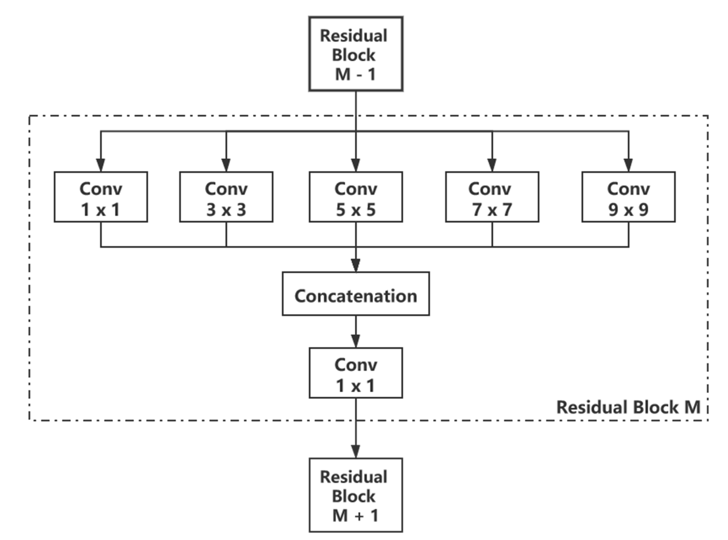
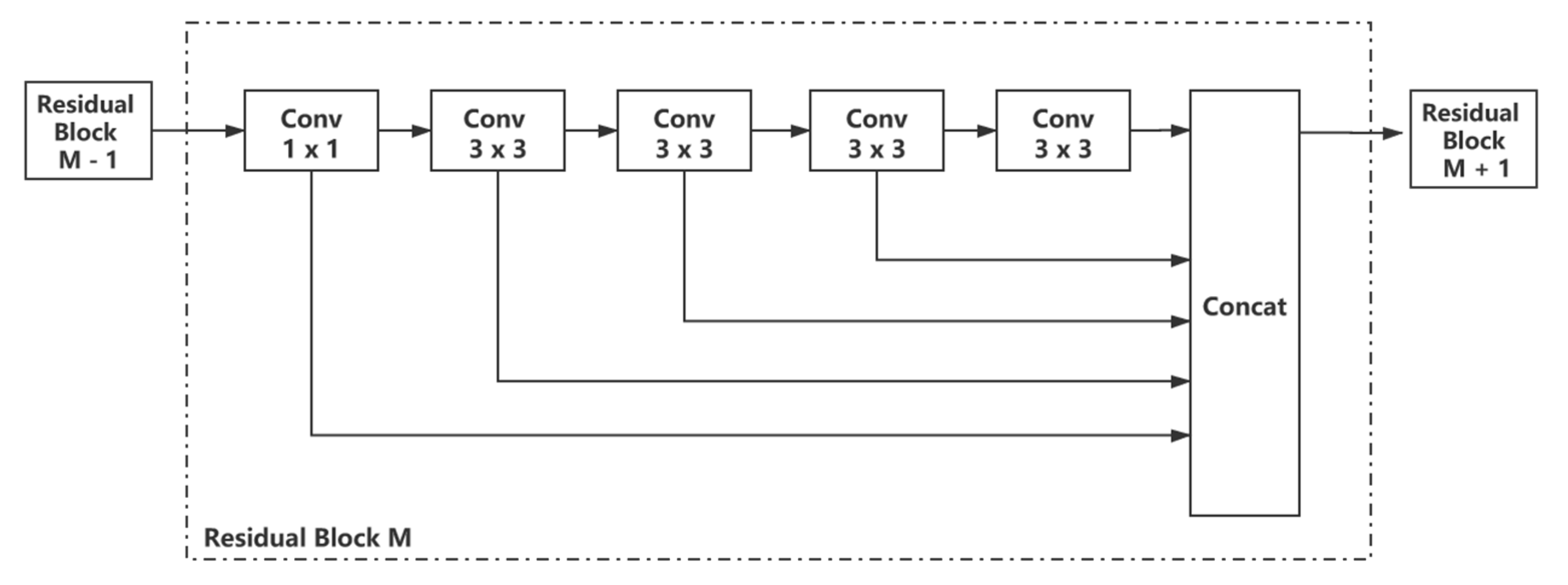
2.4. Single-Core Multiscale Residual Block (SCMSRB)

In existing super-resolution algorithms, multiscale feature extraction is usually performed using convolutional cores of varying size. For instance, the multiscale residual network (MSRN) model proposed by Li, et al. and the GoogleNet Inception architecture [12] both use convolutional cores of varying size (e.g., 1 × 1, 3 × 3 and 5 × 5) for feature extraction from LR images. Large convolutional cores are also used in this process. The number of parameters in each convolutional layer, G, is given by the following equation.
G = K × K × C × D + B
Here, K is the size of the convolutional cores in the convolutional layer, C is the number of channels in the LR image, D is the number of convolutional cores in the convolutional layer, B is the bias of the convolutional core, whose value is identical to that of D. If C and D are fixed, G is directly proportional to the size of the convolutional cores. Hence, the larger the convolutional cores, the greater the number of parameters that must be computed in each convolutional layer.
Factorized convolution [17,18] is the decomposition (factorization) of large convolutional cores into a number of small, connected convolutional cores of the same size. The purpose of this process is to reduce the number of parameters in the convolutional cores and the computational complexity of the algorithm. In this way, a ( 2 K + 1 ) × ( 2 K + 1 ) × D convolutional core can be factorized into K connected 3 × 3 × D convolutional cores. Given an input feature map with C channels, if the unfactorized convolutional core is F R ( ( 2 K + 1 ) × ( 2 K + 1 ) × D ) and M R ( 3 × 3 × D × K ) is the factorized convolutional core, factorization will decrease the number of parameters by H, which is given by
H = [ ( F × C ) ( M × C ) ] F × C
Here, H is proportional to the size of the unfactorized convolutional core, F. In other words, the larger the convolutional core, the greater the decrease in the number of parameters.
Based on multicore multiscale residual blocks (MCMSRBs), we propose the single-core multiscale residual block. The architecture of MCMSRB and its improved derivative, SCMSRB, are shown in Figure 2 and Figure 3, respectively.
In the SCMSRB, N small and identically sized cascaded-residual convolutional cores are used for multiscale feature extraction. The extracted features are then fused by a concatenation operation and reassembled in one dimension, thus enabling multiscale feature extraction from LR images of liquid metal specimens. Each convolutional core generates 64 convolutional feature maps; after the feature maps have been concatenated, a 1 × 1 × 64 convolutional core is used to perform feature mapping and dimension reduction. The multiscale fused feature map from the SCMSRB is then used as input for the next SCMSRB, which extracts additional detail from the LR image. To improve the expressivity of the network model and increase its nonlinearity, a PReLU activation layer is placed after the convolutional layers. The inside of the SCMSRB is expressed by the following mathematical formula.
f 1 × 1 = σ ( w 1 × 1 F 0 + B 1 × 1 )
f 1 3 × 3 = σ ( W 1 3 × 3 F 0 + B 1 3 × 3 )
f N 3 × 3 = σ ( W N 3 × 3 f N 1 3 × 3 + B N 3 × 3 )
Here, f1×1 and f3×3 represent feature extraction from 1 × 1 and 3 × 3 convolutional cores in the SCMSRB, respectively, while N is the number of convolutional cores in the SCMSRB.
F SCB M = f 1 × 1 + i = 1 N f i 3 × 3
F SCB M = σ ( W 2 1 × 1 F SCB M + B 2 1 × 1 )
Here, F SCB M represents the feature extraction of the Mth SCMSRB after reduction in dimensionality by the convolutional layer. W and B represent the 1 × 1 convolutional layer and bias, respectively.
σ ( x ) = max ( a x , x )
σ(x) is the PReLU activation function, which takes values of a ∈ [0,1].

2.5. Upsampling Construction

To generate the global fused feature map, a residual network is used to fuse the LR image with the fused feature map from all SCMSRBs. This is inputted into the subpixel convolution layer [8] for upsampling to obtain the High Resulotion (HR) image. Since the subpixel convolution layer simply arranges the pixels and does not perform any true convolution operations, this arrangement improves the efficiency of the network. The computations performed by the subpixel convolution layer are shown below.
F up = φ ( P S ( W F G F F + B ) )
φ = sinh ( x ) cosh ( x ) = e x e x e x + e x
Here, PS denotes the dimension transformation operation, which transforms the H × W × C r 2 feature map into the rH   ×   rW   ×   C HR images. W and B represent the network weight parameter and bias vector, respectively. φ represents the tanh activation function, which performs nonlinear operations on the up-sampling output.

2.6. Reconstruction

The up-sampled feature map is reconstructed using a 3 × 3 × 3 convolutional layer to obtain a reconstructed image, I H R . It is expressed by the following mathematical formula.
I H R = W F up + B
Here, W and B represent the convolution kernel and bias used by the 3 × 3 reconstruction layer, respectively, and I H R represents the reconstructed HR image.

3. Experimental Process

3.1. Experimental Environment
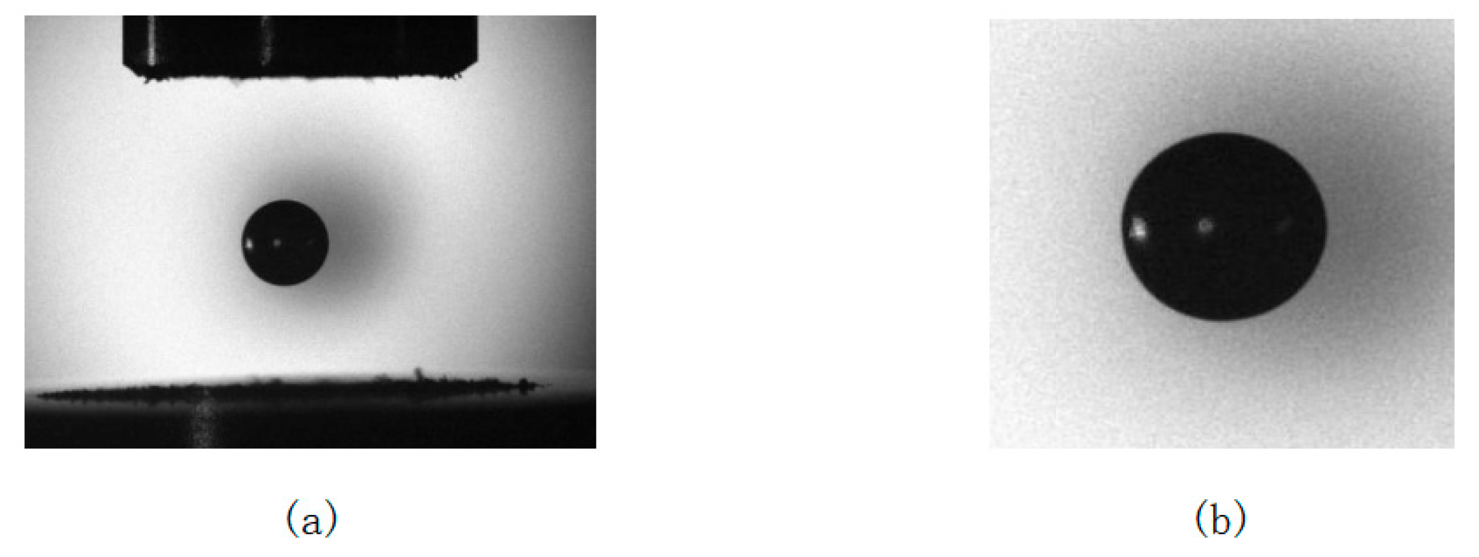
The computer used for this experiment was equipped with an Intel Core i7-9750H CPU running at 2.60 GHz, NVIDIA GeForce GTX 1070 GPU, and 16 GB of RAM. The software environment consisted of the 64-bit Windows 10 operating system, CUDA Toolkit 8.0, CUDNN 7.6.5, and the TensorFlow deep learning framework.

3.2. Dataset

This research topic is based on the study of the liquid metal sample melt under the condition of deep supercooling. The datasets used contain images of the deep supercooled sample melts suspended in the vacuum suspension equipment. There are 50 high-definition images of the deep supercooled melts of the liquid metal samples, as shown in Figure 4a. The image of the droplet part at the central position in the figure is intercepted as a target image for subject research, and the size of the intercepted image is 280 × 280, as shown in Figure 4b. Owing to the high cost of obtaining datasets, we expand the 50 high-definition images by 90°, 180° and 270° rotations of each image and scale them at 0.9, 0.8 and 0.7; the expanded dataset contains a total of 350 high-definition images, numbered from 1 to 350. The datasets numbered 1 to 300 are used as the training sets, those numbered 301 to 325 are used as verification sets, and those numbered 326 to 350 are used as test sets. At the training stage, each image in the training set is down-sampled by 2, 3, and 4 times. Subsequently, the down-sampled images are interpolated to the target image resolution by applying bicubic interpolation, and the enlarged LR images are cut into image blocks at a pixel size of 17 × 17 without overlapping. Furthermore, the high-resolution melt images are cropped in the same manner; finally, the image blocks are formed into high-resolution and LR data pairs, which are used as the input of the network.

3.3. Training Details

The Adam optimization [19,20] algorithm was used to optimize the model’s parameters during the training phase, with its momentum and weight decay parameters set to 0.9 and 0.0001, respectively. Training was performed with a fixed learning rate of 0.0001, and the training process was terminated when training loss reached 0.00001. “SAME” padding was used during the training process to ensure that the size of the feature maps remained invariant.
As the aim of the training process was to learn an end-to-end mapping between LR and HR images, the training set was divided into N LR-HR image pairs, that is, { I LR i , I HR i } i = 1 N , and the network was made to learn the residual image between the LR and HR images. Parameter learning was performed using the mean square error (MSE) [20] between the outputted image and residual image of the image pair. MSE is given by the following equation.
L ( θ ) = min θ 1 2 N i = 1 N | | F ( x i , θ ) y i | | 2
Here, L is the loss function, θ is the parameter to be trained, N is the total number of training sets, F ( x i , θ ) and y i represent the reconstructed image and the corresponding HR image, respectively.

3.4. Evaluation Criteria

Here, two objective metrics, the peak signal to noise ratio (PSNR) and structural similarity index measure (SSIM), are used to objectively evaluate the efficacy of a few super-resolution algorithms in the reconstruction of liquid-metal droplet images. PSNR represents the fidelity of the reconstructed image with respect to the original image; the higher the PSNR value, the lower the loss in fidelity and the greater the image quality. SSIM is an objective measure of similarity based on three characteristics: luminance, contrast, and structure. Unlike PSNR, which compares images in a pixel-by-pixel fashion, SSIM can be used to quantify structural differences between a pair of images. The greater the SSIM value, the more similar the images and the higher the image quality. The equations for PSNR and SSIM are shown below.
P S N R ( y ^ , y ) = 10 log 10 ( 2 n 1 ) 2 M S E ( y ^ , y )
where n is the maximum number of pixel bits in the image, which typically has a maximum value of 255 in grayscale.
S S I M ( X , Y ) = l ( X , Y ) c ( X , Y ) s ( X , Y )
I ( X , Y ) = 2 μ X μ Y + C 1 μ X 2 + μ Y 2 + C 2
c ( X , Y ) = 2 σ X σ Y + C 2 σ X 2 + σ Y 2 + C 2
s ( X , Y ) = 2 σ X Y + C 3 σ X σ Y + C 3
where X represents the reconstructed HR image, and Y represents the original LR image. Here, μ is the mean value of the image, and σ is the variance of the image. C1, C2 and C3 are constants that prevent the denominator from being zero. The default interval of the SSIM value is [0, 1]. When the value of SSIM approaches 1, the reconstructed image is closer to the HR image.

4. Analysis of Results

4.1. Objective Index Analysis

Reconstruction experiments were performed on liquid-metal droplet images, and the results were evaluated using the two aforementioned objective metrics. Table 1 and Table 2 show the comparison of the results of our SCMSRN algorithm with those of mainstream super-resolution algorithms, including the BICUBIC [21], SRCNN, ESPCN, VDSR and MSRN algorithms, as well as the multicore MSRN (MCMSRN) algorithm shown in Figure 2. The data shown in the tables are averages over all the images that were reconstructed by a given algorithm. Figure 5 illustrates the training convergence curves of the SCMSRN, MSRN and MCMSRN algorithms with a test set that consisted of liquid-metal droplet images with a magnification factor of x2.
Based on Table 1 and Table 2, our SCMSRN algorithm was able to outperform all other algorithms, at all magnification factors. Compared to the similarly sized MSRN algorithm and MCMSRN algorithm, the PSNR of our SCMSRN algorithm was 2.03 dB and 1.58 dB higher when the magnification factor was two, 0.08 dB and 0.04 dB higher when the magnification factor was three, and 0.21 dB and 0.2 dB higher when the magnification factor was four. The improvement in PSNR was most pronounced when the magnification factor was two, and the quality of the reconstruction was also highest at this level of magnification.
In Figure 5, it is shown that the introduction of the SCMSRB increased the speed of convergence and reconstruction performance. After 25 epochs of training, the PSNR of the SCMSRN algorithm reached a stable value. The value of the loss function also stopped decreasing after this point.

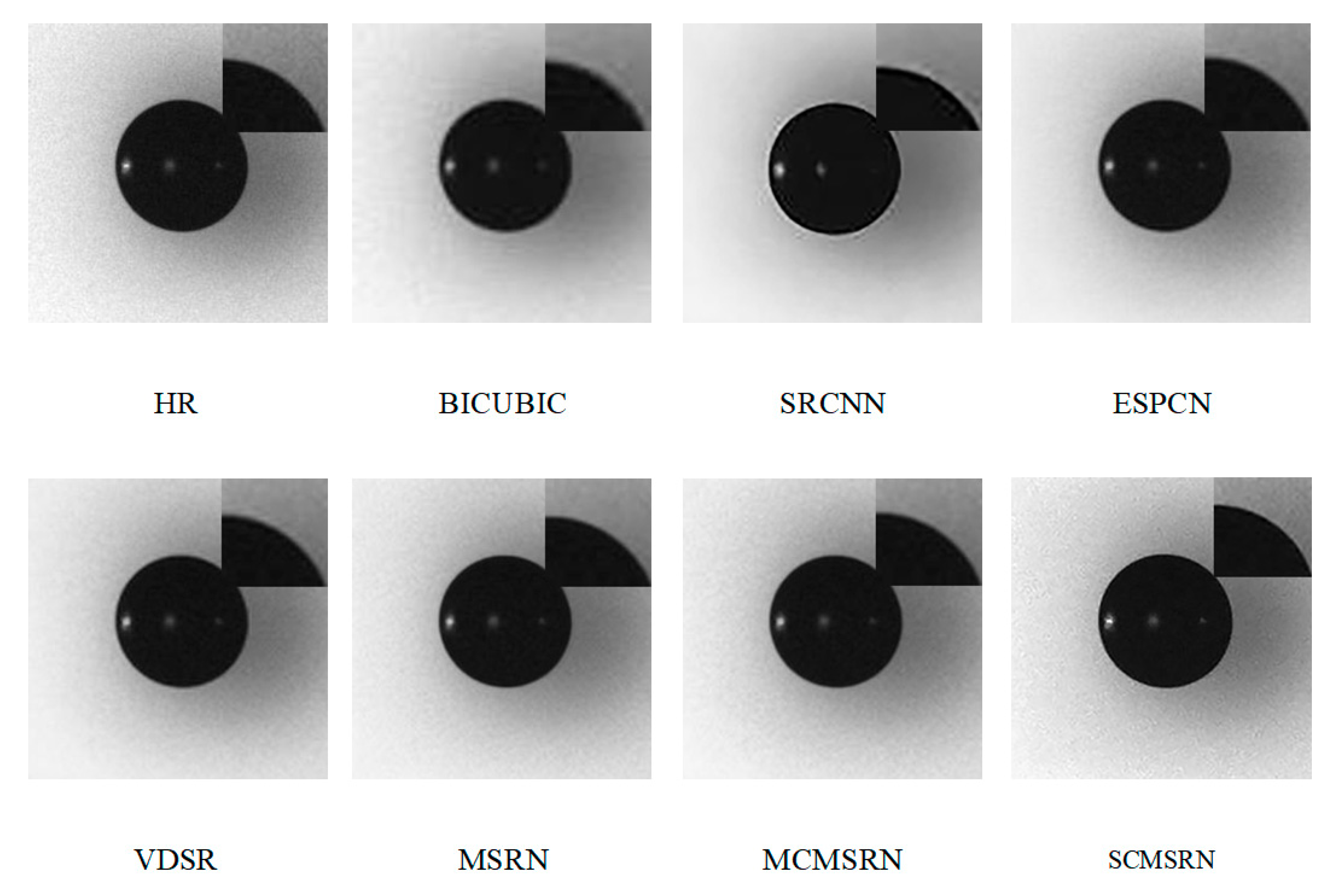
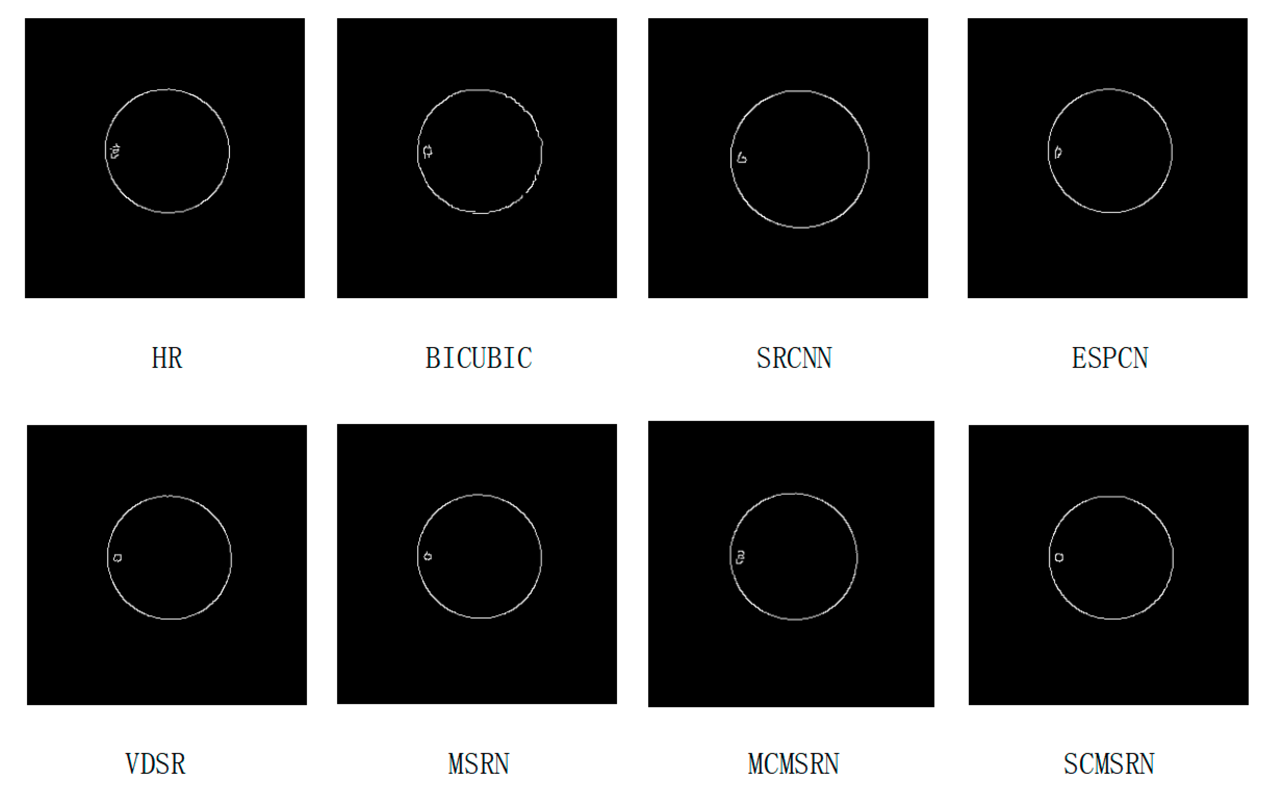
4.2. Visual Effects Analysis

To provide a more intuitive illustration of the results shown by the performance metrics, the image reconstructions were also analyzed in terms of subjective visual acuity. Figure 6 shows the reconstructed and locally magnified images of a 2×-downsampled liquid metal droplet photograph. By comparing the reconstructed images in Figure 6, it is clear that the BICUBIC algorithm was outperformed by all deep learning-based image super-resolution algorithms, as the BICUBIC reconstructions are quite blurry. Compared to the BICUBIC result, the SRCNN algorithm greatly improved image clarity but had a much fuzzier background than the original HR image. The ESPCN and VDSR algorithms were better in terms of background clarity, and the overall clarity of their images were a significant improvement over that of the SRCNN algorithm. The MSRN, MCMSRN and SCMSRN algorithms were able to reconstruct much of the high-frequency detail, and their outputs are a significant improvement over those of the ESPCN and VDSR algorithms in terms of clarity and the definition of the droplet’s edges. In terms of subjective visual quality, our algorithm was able to reconstruct the edges of the droplet more clearly than all other algorithms and produce a result that strongly resembles the original HR image.
For the reconstructed high-resolution image, the Canny operator is used to extract the image contour, and the diameter and area error ratios between the reconstructed image and the original high-resolution image of various algorithms are compared by the method of calculating pixels, so as to verify the various algorithms’ effectiveness in terms of the super-resolution reconstruction of melt images of liquid metal samples.
Figure 7 shows that the algorithm is able to rebuild the samples of liquid metal melt. The Canny operator is utilized to extract the contours of the image; it can be seen that this algorithm rebuilds the image contour information with a richer, more complete outline of the small aperture. This algorithm adopts the hierarchical feature fusion mechanism, which can be extracted from the liquid metal melt sample image in greater detail. It can be seen from Table 3 that the melt image of the liquid metal sample reconstructed by the algorithm in this paper can accurately measure the diameter and area of deep undercooled melt. Based on the original image, the diameter error of the algorithm in this paper is only 0.0103, and the area of error is only two, which is the best among all the comparison algorithms.

4.3. Model Performance Analysis

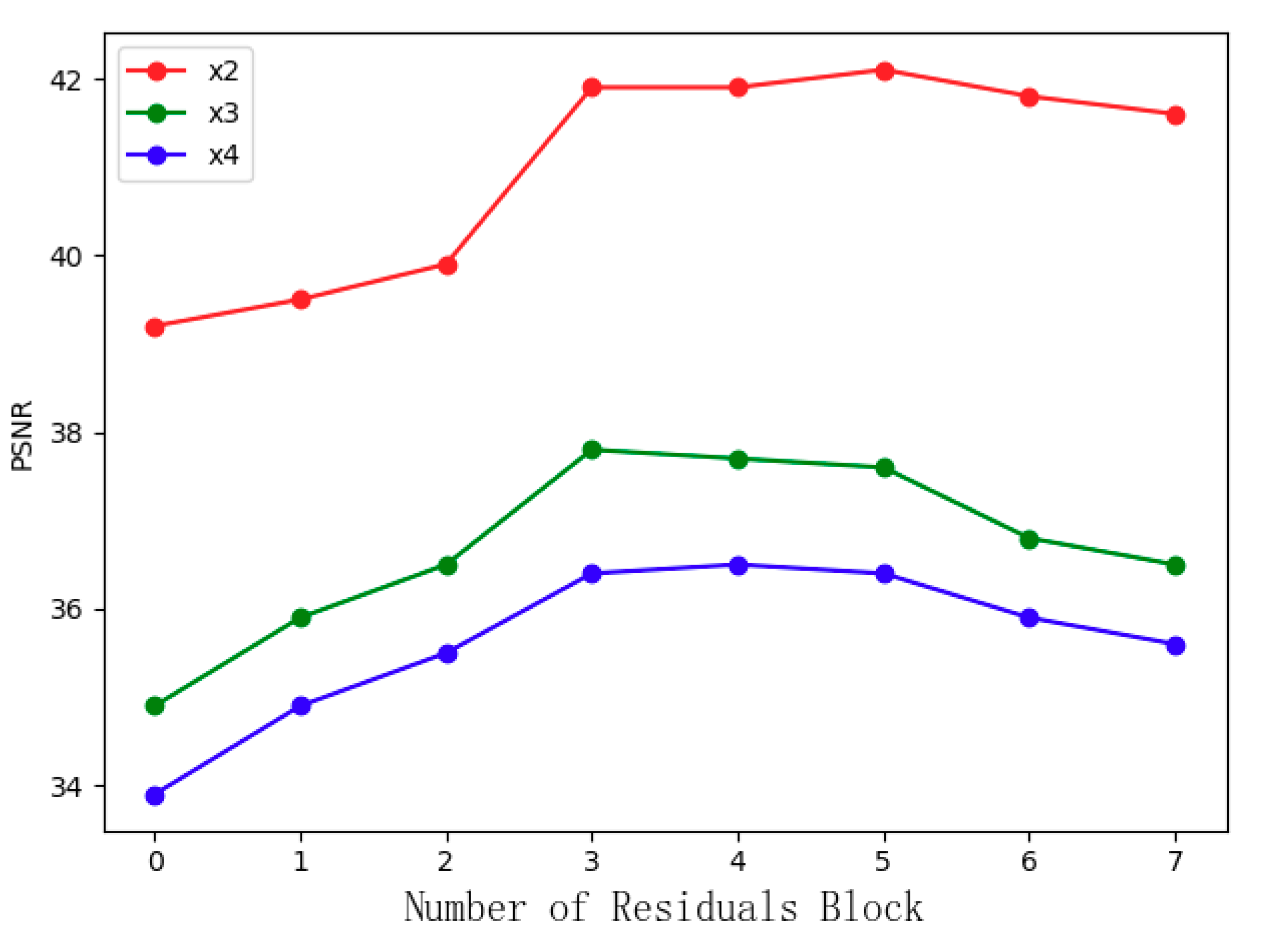
4.3.1. Sub-Module Analysis

By comparing a multitude of model architectures in terms of their efficacy in the super resolution of liquid-metal droplet images, it was found that the number of SCMSRBs was a critical factor for image quality. Network models with 1–8 SCMSRBs were trained to extract and merge 1 × 1, 3 × 3, 5 × 5, 7 × 7 and 9 × 9 residual maps, with each SCMSRB having four cascaded-residual 3 × 3 convolutional cores. In order to ensure the fairness of the experimental results, each model was trained by the training set described in Section 3.2, and the performance was tested on the test set. In the training stage, the learning rate was set as 0.0001, and the number of iterations was 100. Figure 8 illustrates how the number of SCMSRBs affects the super resolution of liquid-metal droplet images by the SCMSRN algorithm, with magnification factors of two, three, and four.
During model training, the network model was only cascaded with one single-core multi-scale residual block. The learning rate was fixed, the peak signal-to-noise ratios (PSNRs) of the test set of the deep undercooling melt images were 41.23 dB, 37.75 dB and 36.12 dB at magnification factors of two, three, and four, respectively. It can be seen that Multiscale feature fusion is a highly effective approach for the super resolution of liquid-metal droplet images.
When cascading 8 SCMSRBs, regardless of the magnification factor, the PSNR value of the sample melt image reconstructed by the model will continue to decrease. This might be attributed to the excessive depth of the model causing convergence difficulties during the training phase; the training loss of this network model only reached 0.00001 after almost 300 epochs of training.
Integrating the effect of model reconstruction under the three magnification factors, when four single-core multi-scale residual blocks are cascaded, the PSNR value of the reconstructed liquid-metal droplet image reaches the peak value at the three magnification factors. Therefore, the number of single-core multi-scale residual blocks M is set to four for the best reconstruction effect.

4.3.2. Performance Analysis

To quantify the efficiency gains that were obtained by the introduction of factorized convolution, MCMSRN and SCMSRN network models were constructed based on the basic modules shown in Figure 2 and Figure 3, respectively, and then assessed in terms of computational efficiency. The metrics used to measure computational efficiency were the number of model parameters (Params), the number of floating-point operations (FLOPs) [21], and training time. The Params metric evaluates the size of the network model, that is, its spatial complexity; the higher the Params value, the greater the spatial complexity. The FLOPs metric assesses the computational complexity of the network model, that is, its time complexity. The lower the FLOPs, the lower the time complexity. Training time is defined as the time taken for the loss function to reach 0.00001 during the training phase. In Figure 5b, it is shown that model loss stabilizes after reaching 0.00001, which indicates that convergence occurs at this point.
In Table 4, it is shown that the SCMSRN algorithm reduced Params by 75%, FLOPs by 75%, and training time by 18 min compared to MCMSRN. Hence, it has been experimentally demonstrated that the SCMSRN algorithm is able to outperform the MCMSRN algorithm in terms of reconstruction quality (while using a smaller number of parameters) and training efficiency.

5. Conclusions

This work proposes an image super-resolution network model for photographic images of liquid metal specimens (droplets), which uses factorized convolution to reduce the tremendous number of model parameters that result from the use of large convolutional cores for multiscale feature extraction and, thus, improves training efficiency for network models of this type. Single-scale multiscale residual blocks are created based on the ideas of residual networks, and they improve the performance of the network model by reducing its number of parameters while enabling the extraction of features with different scales and ensuring sufficient network depths. In liquid-metal droplet image reconstruction experiments, our network model outperformed all current state-of-the-art super-resolution models, in terms of PSNR and SSIM, at three different magnification factors. In the subjective assessment, our network model was able to clearly reconstruct the edges of the liquid metal droplet. The diameter and area that were calculated from the resulting profile were very similar to those derived from the original high-resolution image. Hence, our image super-resolution algorithm can provide accurate data for molten samples poised in simulated gravity-less or microgravity environments, which is significant for the study of novel metastable materials. In the future, we will incorporate an attention mechanism in the design of our network architecture to improve its performance in image reconstruction and, thus, reduce errors in diameter and area measurements.

Author Contributions

For research articles with several authors, the following statements should be used “Conceptualization, X.Z. and K.N.; methodology, Z.Z.; software, Z.Z.; validation, Z.Z., K.H. and S.H.; formal analysis, K.H.; investigation, K.H.; resources, S.H.; data curation, S.H.; writing—original draft preparation, Z.Z.; writing—review and editing, Z.Z.; visualization, Z.Z.; supervision, K.N.; project administration, K.N.; funding acquisition, X.Z. All authors have read and agreed to the published version of the manuscript.

Funding

This research received no external funding.

Data Availability Statement

The data provided in this study can be obtained at the request of the corresponding author. Due to the project is a sub-project in the research, the research is still in progress, this data is not publicly available.

Conflicts of Interest

The authors declare no conflict of interest.

References

  1. Zou, Z.; Luo, X.; Yu, Q. Droplet Image Super Resolution Based on Sparse Representation and Kernel Regression. Microgravity Sci. Technol. 2018, 30, 321–329. [Google Scholar] [CrossRef]
  2. Luo, X.H.; Chen, L. Investigation of microgravity effect on solidification of medium-low-melting-point alloy by drop tube experiment. Sci. China Ser. E Technol. Sci. 2008, 51, 1370–1379. [Google Scholar] [CrossRef]
  3. Dou, R.; Zhou, H.; Liu, L.; Liu, J.; Wu, N. Development of high-speed camera with image quality evaluation. In Proceedings of the 2019 IEEE 8th Joint International Information Technology and Artificial Intelligence Conference (ITAIC), Chongqing, China, 24–26 May 2019; pp. 1404–1408. [Google Scholar] [CrossRef]
  4. Niu, X. An Overview of Image Super-Resolution Reconstruction Algorithm. In Proceedings of the 2018 11th International Symposium on Computational Intelligence and Design (ISCID), Hangzhou, China, 8–9 December 2018; pp. 16–18. [Google Scholar] [CrossRef]
  5. Li, K.; Yang, S.; Dong, R.; Wang, X.; Huang, J. Survey of single image super-resolution reconstruction. IET Image Process. 2020, 14, 2273–2290. [Google Scholar] [CrossRef]
  6. Dong, C.; Loy, C.C.; He, K.; Tang, X. Image Super-Resolution Using Deep Convolutional Networks. IEEE Trans. Pattern Anal. Mach. Intell. 2016, 38, 295–307. [Google Scholar] [CrossRef] [PubMed] [Green Version]
  7. Shi, W.; Caballero, J.; Huszár, F.; Totz, J.; Aitken, A.P.; Bishop, R.; Rueckert, P.; Wang, Z.; Huszr, F. Real-time single image and video super-resolution using an efficient sub-pixel convolutional neural network. In Proceedings of the 2016 IEEE Conference on Computer Vision and Pattern Recognition, Las Vegas, NV, USA, 26 June–1 July 2016; pp. 1874–1883. [Google Scholar]
  8. He, K.; Zhang, X.; Ren, S.; Sun, J. Deep Residual Learning for Image Recognition. In Proceedings of the IEEE Conference on Computer Vision and Pattern Recognition (CVPR), Las Vegas, NV, USA, 26 June–1 July 2016. [Google Scholar]
  9. Kim, J.; Lee, J.K.; Lee, K.M. Accurate Image Super-Resolution Using Very Deep Convolutional Networks. In Proceedings of the IEEE Conference on Computer Vision and Pattern Recognition (CVPR), Las Vegas, NV, USA, 26 June–1 July 2016. [Google Scholar]
  10. Li, J.; Fang, F.; Mei, K.; Zhang, G. Multi-scale Residual Network for Image Super-Resolution. In Proceedings of the 15th European Conference on Computer Vision (ECCV), Munich, Germany, 8–14 September 2018; pp. 517–532. [Google Scholar]
  11. Szegedy, C.; Vanhoucke, V.; Ioffe, S.; Shlens, J.; Wojna, Z. Rethinking the inception architecture for computer vision. In Proceedings of the IEEE Conference on Computer Vision and Pattern Recognition, Las Vegas, NV, USA, 26 June–1 July 2016; pp. 2818–2826. [Google Scholar]
  12. Szegedy, C.; Liu, W.; Jia, Y.; Sermanet, P.; Reed, S.; Anguelov, D.; Erhan, D.; Vanhoucke, V.; Rabinovich, A. Going Deeper with Convolutions. In Proceedings of the IEEE Conference on Computer Vision and Pattern Recognition (CVPR), Boston, MA, USA, 7 June–12 June 2015; pp. 1–9. [Google Scholar]
  13. Viitaniemi, V.; Laaksonen, J. Improving the accuracy of global feature fusion based image categorization. In Proceedings of the International Conference on Semantic and Digital Media Technologies, Genoa, Italy, 5–7 December 2007; Springer: Berlin/Heidelberg, Germany, 2007; pp. 1–14. [Google Scholar]
  14. Simonyan, K.; Zisserman, A. Very Deep Convolutional Networks for Large-Scale Image Recognition. arXiv 2014, arXiv:1409.1556. [Google Scholar]
  15. Chollet, F. Xception: Deep Learning with Depthwise Separable Convolutions. In Proceedings of the 2017 IEEE Conference on Computer Vision and Pattern Recognition (CVPR), Honolulu, HI, USA, 21–26 July 2017. [Google Scholar]
  16. Fernando, B.; Fromont, E.; Muselet, D.; Sebban, M. Discriminative feature fusion for image classification. In Proceedings of the 2012 IEEE Conference on Computer Vision and Pattern Recognition, Providence, RI, USA, 16–21 June 2012; pp. 3434–3441. [Google Scholar]
  17. Kingma, D.; Ba, J. Adam: A Method for Stochastic Optimization. arXiv 2014, arXiv:1412.6980. [Google Scholar]
  18. Zhao, H.; Gallo, O.; Frosio, I.; Kautz, J. Loss Functions for Neural Networks for Image Processing. arXiv 2015, arXiv:1511.08861. [Google Scholar]
  19. Köksoy, O. Multiresponse robust design: Mean square error (MSE) criterion. Appl. Math. Comput. 2006, 175, 1716–1729. [Google Scholar] [CrossRef]
  20. Keys, R.G. Cubic convolution interpolation for digital image processing. IEEE Trans. Acoust. Speech, and Signal Process. 1987, 29, 1153–1160. [Google Scholar] [CrossRef] [Green Version]
  21. Molchanov, P.; Tyree, S.; Karras, T.; Aila, T.; Kautz, J. Pruning Convolutional Neural Networks for Resource Efficient Transfer Learning. arXiv 2016, arXiv:1611.06440. [Google Scholar]
Figure 1. The overall structure of the single-core cascaded residual multi-scale feature fusion network.
Make 03 00023 g001
Figure 2. Architecture of a multicore multiscale residual block (MCMSRB).
Make 03 00023 g002
Figure 3. Architecture of the improved single-core multiscale residual block (SCMSRB).
Make 03 00023 g003
Figure 4. Metal droplet datasets. (a) HR image, (b) HR image after cropping.
Make 03 00023 g004
Figure 5. Model convergence analysis diagram x2. (a) PSNR-epochs curve; (b) loss-epochs curve.
Make 03 00023 g005
Figure 6. Comparison of the local effects of various algorithms on the melt image of liquid metal samples x2.
Make 03 00023 g006
Figure 7. Contrast chart of image contours of melt images of liquid metal samples by algorithms x2.
Make 03 00023 g007
Figure 8. Influence of SCRB module number on PSNR.
Make 03 00023 g008
Table 1. The average PSNR of each algorithm on the melt image of the liquid metal sample (dB).
DatasetsScaleBICUBICSRCNNESPCNVDSRMSRNMCMSRNSCMSRN
Test Datasets236.1837.2538.9639.8940.1240.5742.15
334.7635.9837.4236.9037.5937.6337.67
433.3934.5635.8735.6936.2736.2836.48
Table 2. SSIM average value of each algorithm on the melt image of liquid metal samples.
DatasetsScaleBICUBICSRCNNESPCNVDSRMSRNMCMSRNSCMSRN
Test Datasets20.85300.91850.93920.94630.95280.96230.9637
30.82630.84820.88500.87640.88850.88900.8891
40.80730.82780.84310.84070.84670.85120.8517
Table 3. The outline diameter and area of the melt image of the liquid metal sample extracted based on the Canny operator x2.
MethodsDiameterDiameter ErrorAreaArea Error
HR Image124.0011012076.50
BICUBIC123.85720.143912049.027.5
SRCNN123.89520.105912055.021.5
ESPCN123.93690.064212064.012.5
VDSR123.91380.087312059.517
MSRN124.05760.056512087.511
MCMSRN123.97540.025712071.55
SCMSRN124.01140.010312078.52
Table 4. Comparison in terms of computational efficiency.
MethodsParams/kFLOPs/wTrain Time/min
MCMSRN2791.7806.856
SCMSRN694.5200.738
Publisher’s Note: MDPI stays neutral with regard to jurisdictional claims in published maps and institutional affiliations.

