
Deterministic Local Interpretable Model-Agnostic Explanations for Stable Explainability


Department of Electrical, Computer and Biomedical Engineering, Ryerson University, Toronto, ON M5B 2K3, Canada
*
Author to whom correspondence should be addressed.
Mach. Learn. Knowl. Extr. 2021, 3(3), 525-541; https://0-doi-org.brum.beds.ac.uk/10.3390/make3030027
Submission received: 29 May 2021
/
Revised: 24 June 2021
/
Accepted: 27 June 2021
/
Published: 30 June 2021
(This article belongs to the Special Issue Advances in Explainable Artificial Intelligence (XAI))
Abstract
:Local Interpretable Model-Agnostic Explanations (LIME) is a popular technique used to increase the interpretability and explainability of black box Machine Learning (ML) algorithms. LIME typically creates an explanation for a single prediction by any ML model by learning a simpler interpretable model (e.g., linear classifier) around the prediction through generating simulated data around the instance by random perturbation, and obtaining feature importance through applying some form of feature selection. While LIME and similar local algorithms have gained popularity due to their simplicity, the random perturbation methods result in shifts in data and instability in the generated explanations, where for the same prediction, different explanations can be generated. These are critical issues that can prevent deployment of LIME in sensitive domains. We propose a deterministic version of LIME. Instead of random perturbation, we utilize Agglomerative Hierarchical Clustering (AHC) to group the training data together and K-Nearest Neighbour (KNN) to select the relevant cluster of the new instance that is being explained. After finding the relevant cluster, a simple model (i.e., linear model or decision tree) is trained over the selected cluster to generate the explanations. Experimental results on six public (three binary and three multi-class) and six synthetic datasets show the superiority for Deterministic Local Interpretable Model-Agnostic Explanations (DLIME), where we quantitatively determine the stability and faithfulness of DLIME compared to LIME.
1. Introduction
Recent decades have witnessed the rise of Artificial Intelligence (AI) and Machine Learning (ML) in critical domains such as healthcare, criminal justice and finance [1]. In critical domains, sometimes the binary “yes” or “no” answer is not sufficient and questions such as “how” or “where” something occurred is more significant. To achieve transparency, a few interpretable and explainable models have been proposed in recent literature. These approaches can be grouped based on different criterion [1,2,3,4] such as: (i) Model agnostic or model specific; (ii) Local or global; (iii) Local instance-wise or group-wise; (iv) Intrinsic or post hoc; (v) Variable importance or sensitivity analysis; (vi) Features importance or saliency mapping.
Among them, post hoc model agnostic approaches are popular in practice, where the target is to design a separate algorithm that can explain the decision making process of any ML model. LIME [5] is a well-known model agnostic algorithm. LIME is an instance-based explainer, which generates simulated data points around an instance through random perturbation, and provides explanations by fitting a weighted sparse linear model over predicted responses from the perturbed points. The explanations of LIME are locally faithful to an instance regardless of classifier type. However, the random perturbation may result in data and label shift that can mislead the explanations [6]. Furthermore, the process of perturbing the points randomly makes LIME a non-deterministic approach, lacking “stability”, a desirable property for an interpretable model, especially in critical domains. Vilone et al. and Alvarez-Melis et al. [7,8] defined stability as the consistency of similar explanations for the same or similar inputs.
We propose an array of Deterministic Local Interpretable Model-Agnostic Explanations (DLIME) frameworks. DLIME uses the linear regression as an interpretable model while DLIME-Tree uses tree regression to generate explanations. Both DLIME and DLIME-Tree uses Agglomerative Hierarchical Clustering (AHC) to partition the dataset into different groups instead of randomly perturbing the data points around the instance. The adoption of AHC is based on its deterministic characteristic and simplicity of implementation. Furthermore, AHC does not require prior knowledge of clusters and its output is a hierarchy, which is more useful than the unstructured set of clusters returned by flat clustering such as k-means [9]. Once the cluster membership of each training data point is determined, for a new test instance, KNN classifier is used to find the closest similar data points. After that, all data points belonging to the predominant cluster are used to train a simple model (i.e., linear regression and decision tree) to generate the explanations. Utilizing AHC and KNN to generate the explanations instead of random perturbation results in deterministic explanations for the same instance, which is not the case for LIME. We demonstrate this behavior through experiments on six synthetic and six benchmark datasets from the UCI repository [10], where we show both qualitatively and quantitatively how the explanations generated by DLIME are deterministic and stable, as opposed to LIME. Our contributions can be summarized as follows:
- We achieve stability of explanations using AHC and KNN. Stability in our work specifically refers to intensional stability of feature selection method, which can be measured by the variability in the set of features selected.
- We propose an array of DLIME methods to further improve the quality of explanations.
- We perform detailed ablation study to observe the contribution from each component and demonstrate the superiority of the DLIME as compared to LIME.
2. Related Work
For brevity, we restrict our literature review to locally interpretable models, which encourage understanding of learned relationship between input variable and target variable over small regions. Local interpretability is usually applied to justify the individual predictions made by a classifier for an instance by generating explanations.
LIME [5] is one of the first locally interpretable models, which generates simulated data points around an instance through random perturbation, and provides explanations by fitting a sparse linear model over predicted responses from the perturbed points. Ribeiro et al. [11] extended LIME using decision rules. In the same vein, Leave-One-Covariate-Out (LOCO) [12] and Local Rule-based Explanation (LORE) [13] are other popular techniques for generating local explanation models that offer local variable importance measures. Hall et al. [14] proposed an approach to partition the dataset using k-means instead of perturbing the data points around an instance being explained. The default implementation of k-means picks a centroid randomly, which makes this approach non-deterministic. Hu et al. [15] proposed an approach to partition the dataset using a supervised tree-based approach. Katuwal et al. [16] used LIME in precision medicine and discussed the importance of interpretablility to understand the contribution of important features in decision making.
Robnik-Šikonja [17] proposed a method to decompose the predictions of a classifier on individual contribution of each feature. This methodology is based on computing the difference between original predictions and predictions made by eliminating a set of features. Lundberg et al. [18,19] have demonstrated the equivalence among various local interpretable models [20,21,22] and also introduced game theory based approaches to explain the model named SHAP (SHapley Additive exPlanations) and TreeExplainer. TreeExplainer is a model specific approach that utilizes SHAP values to explain tree-based models only. Baehrens et al. [23] proposed an approach to yield local explanations using the local gradients that depict the movement of data points to change its expected label. A similar approach was used in [24,25,26,27] to explain and understand the behaviour of image classification models.
One of the issues of the existing locally interpretable models is lack of “stability”. Gosiewska et al. [28] defined it as “explanation level uncertainty”, where the authors showed that explanations generated by different locally interpretable models have an amount of uncertainty associated with it due to the simplification of the black box model. In this paper, we address this issue at a more granular level. The basic question that we want to answer is: can explanations generated by a locally interpretable model provide consistent results for the same instance while generating quality explanations? As we will see in the experimental results section, due to the random nature of perturbation in LIME, for the same instance, the generated explanations can be different, with different selected features and feature weights. Generating inconsistent explanations are particularly troublesome for critical application areas such as healthcare. This can reduce the healthcare practitioner’s trust in the ML model. Hence, our target is to increase the stability of the interpretable model. Stability in our work specifically refers to intensional stability of feature selection method, which can be measured by the variability in the set of features selected [29,30]. Measures of stability include average Jaccard similarity and Pearson’s correlation among all pairs of feature subsets selected from different training sets generated using cross validation, jacknife or bootstrap.
A preliminary version of DLIME was presented by us [31] (peer reviewed but not archived). We further extend the work here through (Source code will be available at 24 June 2021 https://github.com/rehmanzafar/dlime_experiments):
- Results on DLIME vs. LIME, DLIME-Tree vs. LIME: The preliminary results presented in the workshop only reported DLIME vs. LIME. The new tree-based version provides better results.
- Further quantification of performance: We computed various statistical evaluation metrics to quantify the performance of the proposed algorithm. We provide comparative results with all features used in the original model and simpler model with selected features by DLIME and LIME.
- Quality of Explanations: We computed the quality of the explanations. Quality computes the closeness among the coefficients of an interpretable model and the original model while stability computes the consistency of the generated explanations.
- Additional Visualization of Explanations: The preliminary results only showed a bar chart that could not show features with zero contributions, which might be useful when selecting features to omit from raw data. In the submitted work, we resolved this limitation by taking advantage of scatter plots.
- Ablation Studies: We perform detailed ablation studies to observe the contribution from each component and demonstrate the superiority of the DLIME as compared to LIME.
3. Methodology
Before explaining DLIME, we briefly describe the LIME framework. LIME is a surrogate model that is used to explain the predictions of any opaque model individually. The objective of LIME is to train surrogate models locally and explain an individual prediction.
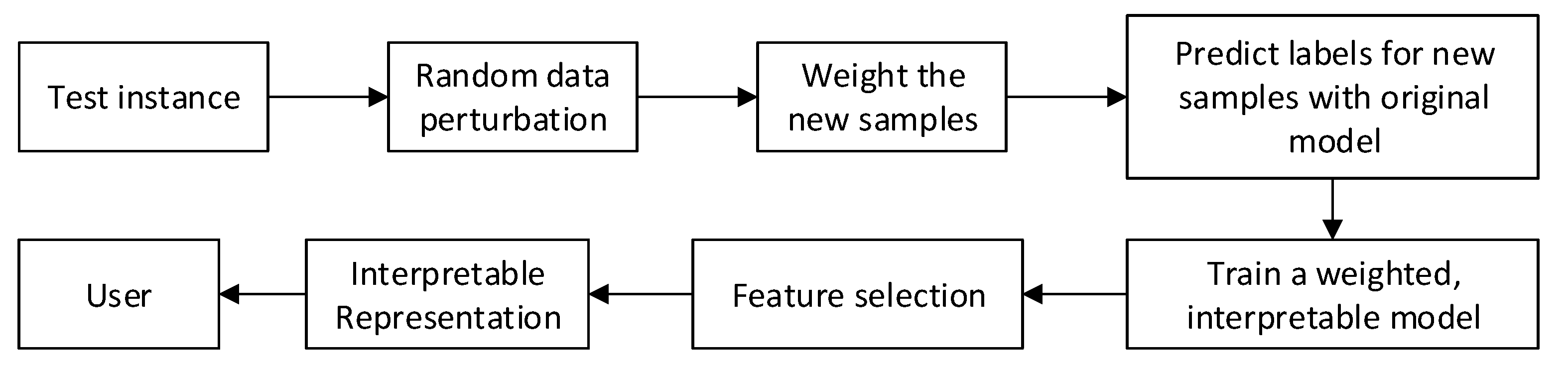
Figure 1 shows a high level block diagram of LIME. It generates a synthetic dataset by randomly permuting the samples around an instance from a normal distribution, and gathers corresponding predictions using the opaque model to be explained. Then, on this perturbed dataset, LIME trains an interpretable model (e.g., linear regression). Linear regression maintains relationships amongst variables which are dependent such as y and multiple independent attributes such as by utilizing a regression line , where “” is intercept, “” is slope of the line and . This equation can be used to predict the value of target variable from given predictor variables. In addition to that, LIME takes as an input the number of important features to be used to generate the explanation, denoted by . The lower the value of , the easier it is to understand the model. There are several approaches to select the important features such as (i) backward or forward selection of features and (ii) Highest weights of linear regression coefficients. LIME uses the forward feature selection method for small datasets which have less than 6 attributes, and highest weights approach for higher dimensional datasets.
As discussed before, a drawback of LIME is the “instability” of generated explanations due to the random sampling process. Because of the randomness, the outcome of LIME is different when the sampling process is repeated multiple times, as shown in experiments. The process of perturbing the points randomly makes LIME a non-deterministic approach, lacking “stability”, a desirable property for an interpretable model, especially in critical domains. Another limitation of LIME is, it may fail to capture the relationship among attributes if the dataset is locally non-linear because it uses linear regression to generate explanations [32].
3.1. DLIME
In this section, we present our proposed Deterministic Local Interpretable Model-Agnostic Explanations (DLIME) model, where the target is to generate stable explanations for a test instance. Figure 2 shows a block diagram of DLIME framework.
The key idea behind DLIME is to utilize AHC to partition the training dataset into different clusters. Then, to generate a set of samples and corresponding predictions (similar to LIME), instead of random perturbation, KNN is first used to find the closest neighbors to the test instance. The samples with the majority cluster label among the closest neighbors are used as the set of samples to train the linear regression model that can generate the explanations. The different components of the proposed method are explained further below.
3.1.1. Neighborhood Selection
A significant number of neighborhood selection methods have been proposed recently [5,14,33,34]. All of these approaches are based on random perturbations. The randomness of perturbed data points makes interpretable models non-deterministic. The random behaviour can be disabled by setting the seed value in the algorithm. However, random sampling can suffer shift in data and labels that can mislead the explanations. The data generated with random sampling can be significantly different from its original source [6,35].
Therefore, to produce a meaningful local explanation, it is crucial to correctly sample data around an instance that is being explained. Particularly, the local data needs to be sampled from the same distribution that generated the original data. The simplest way is to use the original data by filtering it based on class labels. This approach is not applicable if the data is high dimensional and multiple regions have the same class label. It will filter out the farthest regions with same label as well that can mislead the explanations. Therefore, we used nearest neighbours and AHC based approaches to select the neighbourhood. Algorithm 1 formally presents the neighborhood selection approach.
| Algorithm 1: Neighbourhood Selection. |
 |
3.1.2. Hierarchical Clustering
Hierarchical clustering is a commonly used unsupervised ML approach due to better computational stability [36], which generates a binary tree with cluster memberships from a set of data points. The leaves of the tree represent data points and nodes represent nested clusters of different sizes. There are two main approaches to hierarchical clustering: divisive and AHC. AHC follows the bottom-up approach and divisive clustering uses the top-down approach to merge the similar clusters. This study uses the traditional AHC approach as discussed in [37]. Initially, it considers every data point as a cluster (i.e., it starts with N clusters and merge the most similar groups iteratively until all groups belong to one cluster). AHC uses euclidean distance between closest data points or clusters mean to compute the similarity or dissimilarity of neighbouring clusters [38].
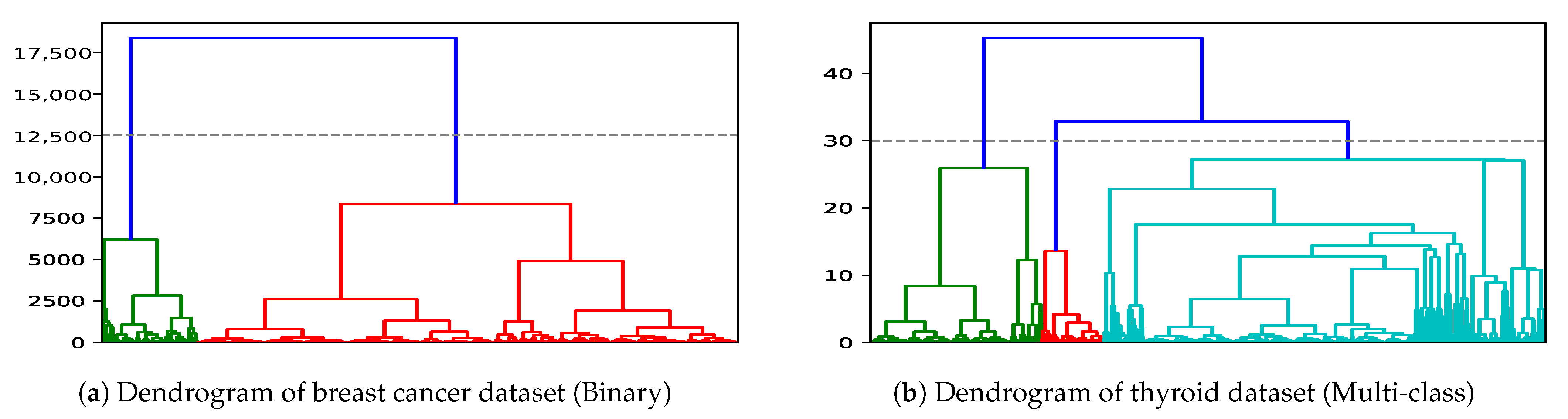
One important step to use AHC for DLIME is determining the appropriate number of clusters C. AHC is in general visualized as a dendrogram. In the dendrogram, each horizontal line represents a merge and the y-coordinate of it is the similarity of the two merged clusters. A vertical line shows the gap between two successive clusters. By cutting the dendrogram where the gap is the largest between two successive groups, we can automatically determine the value of C. As we can see in Figure 3a, the largest gap between two clusters is at level 2 for the breast cancer dataset, which has 2 classes. For multi-class problems, the value of C will change as shown in Figure 3b, utilizing the Thyroid dataset from the UCI repository. The dotted line in Figure 3b represents a cutoff point to determine the value of C. From the dendrogram in Figure 3b, it can be observed that is the correct choice for the 3-class Thyroid dataset.
3.1.3. K-Nearest Neighbor (KNN)
Similar to other clustering approaches, AHC does not assign labels to new instances. Therefore, KNN is trained over the training dataset to find the indices of the neighbours and predict the label of new instance. KNN is a simple classification model based on Euclidean distance [39]. It computes the distance between training and test sets. Let be an instance that belongs to a training dataset of size n where, i in range of . Each instance has m features (,). In KNN, the Euclidean distance between new instance x and a training instance is computed. After computing the distance, indices of the k smallest distances are called k -nearest neighbors. Finally, the cluster label for the test instance is assigned the majority label among the k-nearest neighbors. After that, all the data points belonging to the predominant class is used to train a linear regression model to generate the explanations. In our experiments, was used, as higher values of k did not make a difference in the results.
A natural question that may arise from the proposed framework is: what if we do not perform any clustering, and apply KNN directly instead? Applying KNN directly may result in highly noisy output, especially for overlapping classes. In Section 4, we present ablation studies to validate that AHC is a required step to obtain quality explanations.
3.1.4. DLIME-Tree
Tree-based models are more interpretable, accurate and usually outperform other ML models on tabular data, where each and every feature is momentous [19]. Tree-based models are robust to outliers and outperform linear models by dividing it into various subsets. Therefore, tree-based models are handy when there are complex interactions among the independent and dependent features. In addition to the linear regression-based DLIME, in this work we present a tree-based explainer that we call DLIME-Tree. We used a Random Forest Regressor (RFR) with 10 estimators, 10 maximum depth, 10 maximum features and disabling the random behaviour. RFR is a meta estimator that constructs many decision trees on various subsets of datasets and uses averaging to avoid over-fitting and improve the predicting accuracy of the model. In [19], authors introduced non-linearity in a mortality dataset to demonstrate that tree-based methods are robust to capture the complex interactions among the attributes while data is non-linear. Therefore, we decided to proceed with tree-based regression in our algorithm instead of linear regression.
Two popular methods to explain a tree-based model are (i) Tree-interpreter [40] and (ii) Tree-explainer [19]. Both of these approaches are model-specific and compute the feature importance to generate the explanations. The way of computing feature importance is the only difference among these two approaches. Tree-explainer explains a prediction by using the shapely values to approximate the contribution of features over all possible feature subsets. On the other hand, Tree-interpreter follows the decision path and attributes changes in prediction to each feature along the prediction path. Tree-interpreter uses Equation (1), where T is the number of trees, is the average of bias from the complete dataset and K is the total number of features.
In our work, we continue with Tree-interpreter as its output is decomposed in bias and features contribution (i.e., where, is the contribution of feature and ). It is very similar to a linear equation that can be easily compared with linear regression based model explainers.
Utilizing the notations introduced above, Algorithm 2 formally presents the proposed DLIME and DLIME-Tree frameworks (the isTree boolean on line 6 differentiates DLIME from DLIME-Tree).
| Algorithm 2: Deterministic Local Interpretable Model-Agnostic Explanations. |
 |
4. Experiments
The most recent literature [33,41,42] shows that synthetic data has various advantages over the real-world data in performing ablation studies and evaluating the machine learning models in a controlled environment. Therefore, we generated six synthetic datasets as discussed in [33], a recent work on explainable models. Furthermore, we evaluated DLIME on three binary and three multi-class real-world datasets from the UCI repository. The datasets are described in Table 1.
To evaluate each component of DLIME, respectively, through an ablation study, we employed the following array of DLIME approaches with different settings:
- DLIME utilizes AHC, KNN, and linear regression.
- DLIME-KM utilizes k-means (disabling its random behaviour of picking centroid) and linear regression.
- DLIME-NN utilizes KNN with 50 neighbours and linear regression.
- DLIME-Tree utilizes AHC, KNN, and tree regression.
Each version of DLIME tests whether a specific component has a positive or negative effect on the overall performance. By comparing with DLIME-KM, we demonstrate that AHC is superior to k-means for finding local subspaces. By comparing with DLIME-NN, we demonstrate that clustering is a required step to find accurate local subspaces. Finally, comparing DLIME with DLIME-Tree demonstrates the difference between using linear regression and tree regression to generate explanations.
4.1. Evaluation Metrics
There are different evaluation metrics proposed in the literature and these are broadly categorized into two groups: (i) Objective evaluations and (ii) Human-centered evaluations [7]. The objective evaluations employ objective metrics such as stability and quality of explanations to automate the evaluation of an explainer. However, human-centered evaluations require humans in the loop and utilizes the feedback provided by the humans. We used two objective metrics (stability and quality) to evaluate our framework.
The assessment of the quality of explanations is crucial before deploying an explainable model into production. The evaluation of an interpretable model is a challenging task because of its subjective nature. A few studies have used human participation to evaluate the model. However, utilizing human participants is quite expensive and prone to cognitive biases [43]. Therefore, the importance of evaluating the interpretable models quantitatively is emphasised in [44].
Two main concepts to compute the reliability and correctness of an interpretable model are quality [33] and stability. Quality computes the closeness among the coefficients of an interpretable model and the original model while stability computes the consistency of the generated explanations.
We used logistic regression as our true model to compute the quality of the explanations generated with both DLIME and LIME. Logistic regression is an extension of linear regression that uses a sigmoid function for binary classification [2] and One-Vs-The-Rest scheme for multiclass [45]. Similar to linear regression it uses coefficients to produce the results that makes it an interpretable model. The evaluation metric to compute the quality is formally defined in Algorithm 3, where, is a vector of coefficients obtained from the logistic regression (a true model in our case) and is the explanation vector obtained from the explainer (i.e., DLIME or LIME). The quality q of explanation e is measured by using the cosine similarity and quality score is computed by taking the average of q for all instances in the test dataset.
| Algorithm 3: Quality of Explanations. |
 |
4.2. Opaque Models
This section provides a general introduction of the blackbox models used in this study. We trained random forest and neural network by utilizing the scikit-learn package [46]. These models are popular because of their high performance, but hard to explain.
- Random forest is a supervised machine learning algorithm that can be used for both regression and classification [47]. Random forest is a meta estimator that constructs many decision trees on various subsets of datasets and uses averaging to avoid over-fitting and improve the predicting accuracy of the model. The performance of random forest is based on the correlation and strength of each tree. If the correlation between two trees is high, the error will also be high. The tree with the lowest error rate is the strength of the classifier.
- Neural network is a biologically inspired supervised machine learning model, which is composed of a large number of highly interconnected neurons working concurrently to resolve particular problems. There are different types of neural networks, among which we picked the popular feed forward artificial neural network. It typically has multiple layers and is trained with the backpropagation. The particular neural network we utilized has two hidden layers. The first hidden layer has five hidden units and the second hidden layer has two hidden units.
For both opaque models, of the data is used for training and the remaining of the data is used for evaluation. Here, it is worth mentioning that both neural network and random forest models scored over 90% accuracy on each dataset, which is reasonable. Their performance can be improved by hyper parameter tuning. However, our aim is to produce deterministic explanations; therefore, we have not spent additional effort to further tune these models.
After training these opaque models, both LIME (default python implementation) and DLIME were used to generate explanations for all test instances. For each instance, 10 iterations of both algorithms were executed to determine the quality and stability.
4.3. Results
This section presents the results of DLIME framework proposed in the study. We have utilized only one test instance in Figure 4 and Figure 5 to highlight the instability associated with explanations generated with LIME. Table 2 shows the average Features Stability Index (FSI) score for the complete dataset. The FSI is the average Jaccard distance computed after 10 iterations for each instance in the test dataset to demonstrate the stability of DLIME.
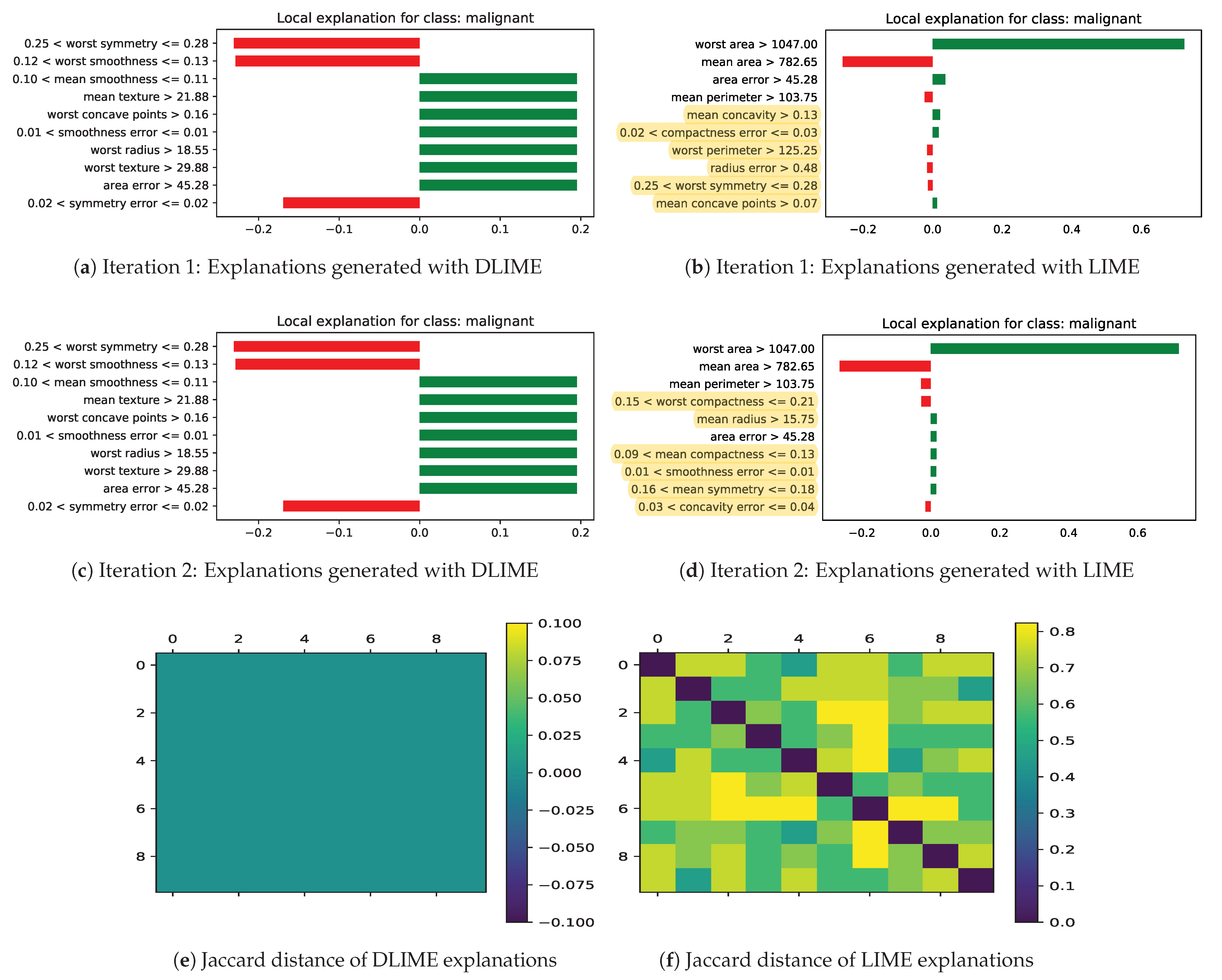
Figure 4 shows the results for two iterations of explanations generated by DLIME and LIME for a randomly selected test instance with the trained neural network on the breast cancer dataset. On the left hand side in Figure 4a,b are the explanations generated by DLIME, and on the right hand side Figure 4b,d are the explanations generated by LIME. The red bars in Figure 4a, shows the negative coefficients and green bars shows the positive coefficients of the linear regression model. The positive coefficients shows the positive correlation among the dependent and independent attributes. On the other hand, negative coefficients shows the negative correlation among the dependent and independent attributes.
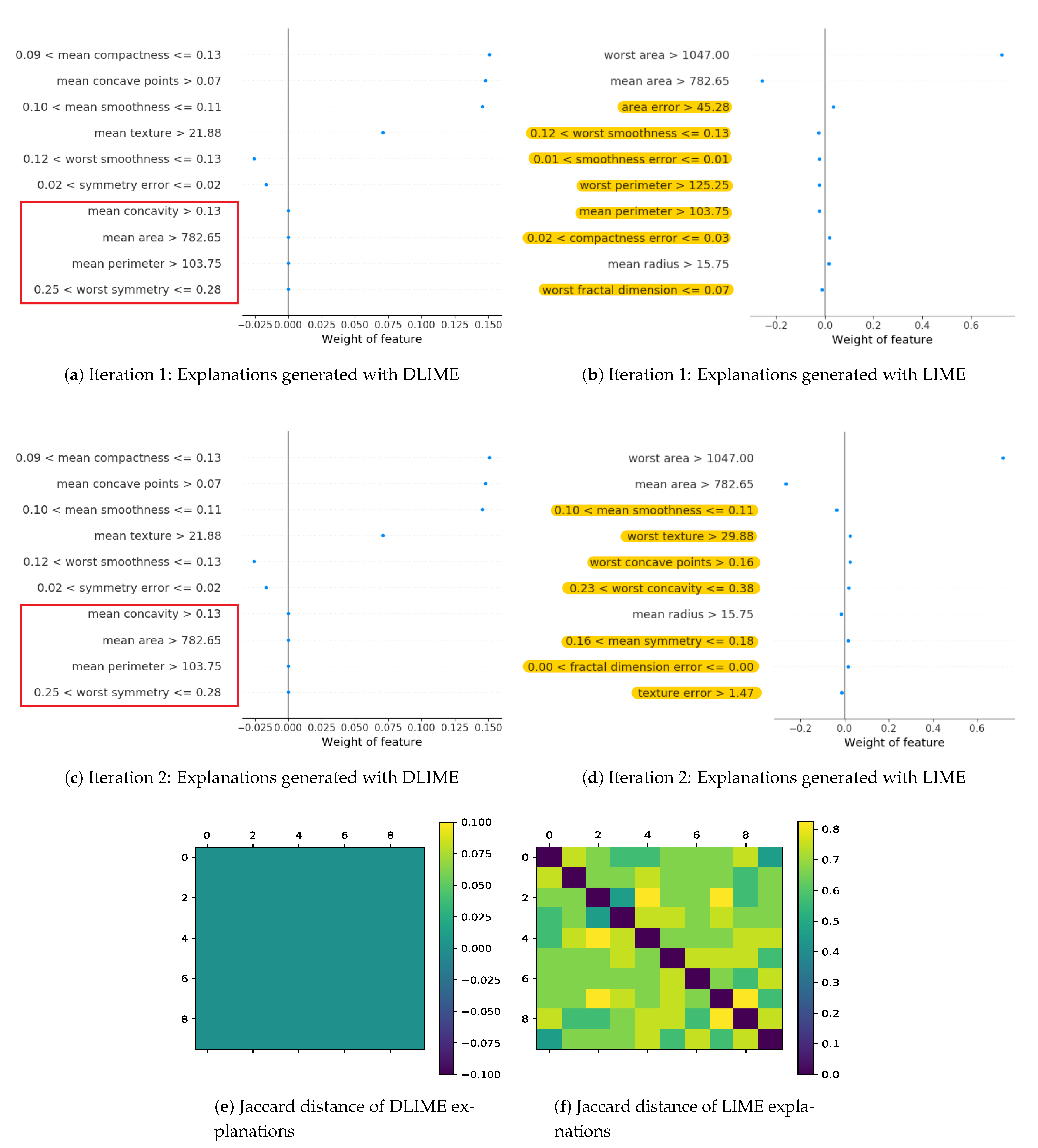
Furthermore, Figure 5 shows the results for two iterations of explanations generated by DLIME-Tree and LIME for a randomly selected test instance with the trained neural network on the breast cancer dataset. Figure 4 and Figure 5 are two different choices of visualizing explanations. Explanations generated with tree-based regression has features with zero contribution that cannot be visualized with bar charts. Therefore, we took advantage of the scatter plot to visualize explanations including features with zero contribution. The vertical line at on all sub figures in Figure 5 represents the zero contribution of the individual features and it also separates the positive and negative coefficients. On the left side of the vertical line, blue dots show the negative coefficients while the right side of the vertical line shows the positive coefficients computed from the RFR model by using Equation (1). From Figure 5a,c, we can observe that the attributes marked by the red outlines are not important in making predictions and can be eliminated from the feature space. By defining a threshold, we can filter features. Explanations with fewer number of features are more understandable and easier to visualize.
As we can see, LIME is producing different explanations for the same test instance. The yellow highlighted attributes in Figure 4b and Figure 5b are different from those in Figure 4d and Figure 5d, respectively. On the other hand, explanations which are generated with DLIME are deterministic and stable as shown in Figure 4a,c and Figure 5a,c. The default implementation of LIME is using 5000 randomly perturbed data points around an instance to generate the explanations. On the other hand, DLIME is using only clusters from the original dataset. For DLIME linear regression, the dataset has fewer number of data points since it is limited by the size of the cluster. Therefore, the explanations generated with LIME and DLIME can be different. However, DLIME explanations are stable, while those generated by LIME are not. In the next sections, we show that the quality and faithfulness of explanations generated by DLIME are also comparable to LIME.
4.3.1. Stability
To further quantify the stability of the explanations, we have utilized Jaccard coefficient in Algorithm 4 where, and are the two sets of explanations. The result of means and are highly similar sets. when , implying that and are highly dissimilar sets. computes the degree of dissimilarity among the sets and . By utilizing the , we have computed the FSI which is the average distance of all explanations generated with both DLIME and LIME, after 10 iterations. Table 2 shows the FSI obtained for DLIME and LIME utilizing the two opaque models on three public datasets. As we can see, in every scenario, the FSI for DLIME is zero, while for LIME it contains significant values, demonstration the stability of DLIME when compared with LIME.
| Algorithm 4: Features Stability Index (FSI). |
 |
Figure 4e,f shows the . It is a matrix. The diagonal of this matrix is 0 that shows the of the explanation with itself and lower and upper diagonal shows the of explanations from each other. Lower and upper diagonal are representing the same information. It can be observed that the in Figure 4e is 0 which means the generated explanations with DLIME are deterministic and stable on each iteration. However, for LIME, as we can see, the contain significant values in Figure 4f, further proving the instability of LIME.
4.3.2. Faithfulness
To further prove that the explanation generated with DLIME is not only stable but also faithful, we computed the quality of the explanations on twelve datasets discussed in Section 4. Table 4 shows the quality of explanations computed by using Algorithm 3 and the statistical significance. To compute the quality of the explanations, a logistic regression model is treated as true model and trained on the training data with all features. To determine the difference in explanations generated with array of methods discussed in Section 4, we performed paired t-tests [48] among the average cosine similarity of best performing model and the rest of the models after 10 iterations. The p-Values of each model are reported in Table 4 for each dataset.
4.3.3. Classification Performance with Selected Features
To further prove that the features selected for explanation generation by DLIME are in fact relevant features, we compare the classification performance on the datasets with respect to the original model, which utilizes all features. Table 3 reports the performance of algorithms by computing the precision, recall, f1-score accuracy and balanced accuracy of both LIME and DLIME. In the context of classification, precision is defined as , where is the number of false positives and is the number of true positives. Similarly, recall is defined as , where the number of false negatives and is the number of true positives. F-1 score is the harmonic mean of recall and precision and defined as . Accuracy is the ratio of true positives and true negative among all samples and defined as where is the number of true negatives. Balanced accuracy computes the specificity and sensitivity of the model, and divides their sum by 2. Sensitivity measure the true positive rate which is the same as recall. However, specificity measures the true negative rate which can be calculated with where, is the number of true negatives.
Table 3 shows that DLIME-Tree outperformed both DLIME and LIME. Among all other approaches, LIME scored the highest recall. However, the recall of LIME may change because it uses random perturbation to explain an instance. However, LIME has lower F1-score and accuracy as compared to both DLIME-Tree and DLIME. Here, it is worth mentioning that, both DLIME-Tree and DLIME generates deterministic explanations while achieving better accuracy and balanced accuracy, making it more trustworthy and stable when compared to LIME.
4.4. Discussion on Quality
In this section, we provide in-depth discussion on the comparative performance of an array of DLIME approaches when compared to LIME. The quality of generated explanations is reported in Table 4 for both binary and multi-class datasets. Each value in these tables is the average quality computed over a complete test set as discussed in Algorithm 3.
Table 4 shows that DLIME and DLIME-Tree outperforms or matches the performance of LIME and other variations of DLIME for almost all datasets. The two exceptions are Synthetic II, where DLIME-KM significantly outperforms the others and Synthetic III, where LIME significantly outperforms the others. A possible reason for these two exceptions could be the quality of local neighbourhood. Here, we identified the ways to generate high quality neighbourhood and it is worth mentioning that good neighbourhood generation is very critical in local post hoc model agnostic explanation methods.
When comparing DLIME to DLIME-Tree, we see that they are very competitive across all the datasets. This shows that regardless of whether a linear or tree explainer is used, DLIME can generate quality explanations. However, tree-based explainers can be more interpretable compared with linear regression based explainers due to their rule- based output. Tree-based explainers produce human-readable rules that are useful for direct understanding of the prediction process and explain the patterns learned from data. On top of that, tree-based explainers are capable of generating global explanations.
Looking at the statistical significance results in Table 4, we see that when DLIME or DLIME-Tree outperforms LIME, the results are also statistically significant (p < 0.05). One notable exception is Synthetic V, where none of the methods are significantly better than the others. This is expected for some datasets, since DLIME-KM and DLIME-NN are minor variations of DLIME created for ablation studies. However, across the datasets, DLIME and DLIME-Tree mostly outperform LIME with statistical significance.
5. Conclusions
In this paper, we propose a deterministic approach to explain the decisions of black box models. Instead of random perturbation, DLIME uses AHC by utilizing KNN to find cluster of data points that are similar to a test instance. Therefore, DLIME can produce deterministic explanations for a single instance by achieving better quality compared to LIME. On the other hand, LIME and other similar model agnostic approaches based on random perturbing may keep changing their explanation on each iteration, creating distrust particularly in the medical domain where consistency is highly necessary.
To evaluate the DLIME, we performed an ablation study by generating six synthetic datasets and also used six real-world (three binary and three multi-class) datasets from the UCI repository. The experiments clearly demonstrate that the explanations generated with all versions of DLIME are deterministic on each iteration, while LIME generates inconsistent explanations. Since DLIME depends on AHC to find similar data points, the number of samples in a dataset may affect the quality of clusters and, consequently, the accuracy and quality of the local predictions. In future, we plan to investigate how to solve this issue while keeping the model explanations deterministic. Furthermore, we would like to explore and investigate the evaluation metrics to evaluate the interpretable models convincingly.
A limitation of objective metrics is the inability to evaluate the qualitative accuracy of explanations generated with different frameworks. As it can be observed, explanations generated with different approaches in Figure 4a, Figure 4b and Figure 5a are different. The difference in generated explanations may raise a question: which explanations are qualitatively more accurate? Despite of the vast variety of notions and methods, it is still an open question that needs to be answered. Since this question requires domain knowledge and is strictly connected to humans, future research should focus on a human-in-the-loop approach as discussed in [7]. In future, we will perform user studies similar to the one performed in LIME [5,49] to answer that question.
Author Contributions
Conceptualization, M.R.Z. and N.K.; methodology, M.R.Z. and N.K.; software, M.R.Z.; validation, M.R.Z. and N.K.; formal analysis, M.R.Z. and N.K.; investigation, M.R.Z. and N.K.; resources, M.R.Z. and N.K.; data curation, M.R.Z.; writing—original draft preparation, M.R.Z. and N.K.; writing—review and editing, M.R.Z. and N.K.; visualization, M.R.Z.; supervision, N.K.; project administration, N.K. Both authors have read and agreed to the published version of the manuscript.
Funding
This work was partially funded by the Natural Science and Engineering Research Council of Canada (NSERC) through the Discovery program (grant #RGPIN-2020-05471).
Institutional Review Board Statement
Not applicable.
Informed Consent Statement
Not applicable.
Data Availability Statement
Not applicable.
Conflicts of Interest
The authors declare no conflict of interest.
References
- Arrieta, A.B.; Díaz-Rodríguez, N.; Del Ser, J.; Bennetot, A.; Tabik, S.; Barbado, A.; García, S.; Gil-López, S.; Molina, D.; Benjamins, R.; et al. Explainable Artificial Intelligence (XAI): Concepts, taxonomies, opportunities and challenges toward responsible AI. Inf. Fusion 2020, 58, 82–115, preprinted in arXiv 2019, arXiv:1910.10045. [Google Scholar] [CrossRef] [Green Version]
- Molnar, C. Interpretable Machine Learning. 2019. Available online: https://christophm.github.io/interpretable-ml-book/ (accessed on 23 March 2020).
- Guidotti, R.; Ruggieri, S. Assessing the Stability of Interpretable Models. arXiv 2018, arXiv:1810.09352. [Google Scholar]
- Plumb, G.; Molitor, D.; Talwalkar, A.S. Model Agnostic Supervised Local Explanations. In Advances in Neural Information Processing Systems; The MIT Press: Cambridge, MA, USA, 2018; pp. 2520–2529. [Google Scholar]
- Ribeiro, M.T.; Singh, S.; Guestrin, C. Why should i trust you?: Explaining the predictions of any classifier. In Proceedings of the 22nd ACM SIGKDD International Conference on Knowledge Discovery and Data Mining, San Francisco, CA, USA, 13–17 August 2016; pp. 1135–1144. [Google Scholar]
- Rahnama, A.H.A.; Boström, H. A study of data and label shift in the LIME framework. arXiv 2019, arXiv:1910.14421. [Google Scholar]
- Vilone, G.; Longo, L. Notions of explainability and evaluation approaches for explainable artificial intelligence. Inf. Fusion 2021, 76, 89–106. [Google Scholar] [CrossRef]
- Alvarez-Melis, D.; Jaakkola, T.S. Towards Robust Interpretability with Self-Explaining Neural Networks. In Proceedings of the 32nd International Conference on Neural Information Processing Systems (NIPS’18); Curran Associates Inc.: Red Hook, NY, USA, 2018; pp. 7786–7795. [Google Scholar]
- Manning, C.D.; Raghavan, P.; Schütze, H. Introduction to Information Retrieval; Cambridge University Press: New York, NY, USA, 2008. [Google Scholar]
- Dua, D.; Graff, C. UCI Machine Learning Repository; University of California: Irvine, CA, USA, 2017. [Google Scholar]
- Ribeiro, M.T.; Singh, S.; Guestrin, C. Anchors: High-precision model-agnostic explanations. In Proceedings of the Thirty-Second AAAI Conference on Artificial Intelligence, New Orleans, LA, USA, 2–7 February 2018. [Google Scholar]
- Lei, J.; G’Sell, M.; Rinaldo, A.; Tibshirani, R.J.; Wasserman, L. Distribution-free predictive inference for regression. J. Am. Stat. Assoc. 2018, 113, 1094–1111. [Google Scholar] [CrossRef]
- Guidotti, R.; Monreale, A.; Giannotti, F.; Pedreschi, D.; Ruggieri, S.; Turini, F. Factual and Counterfactual Explanations for Black Box Decision Making. IEEE Intell. Syst. 2019, 34, 14–23. [Google Scholar] [CrossRef]
- Hall, P.; Gill, N.; Kurka, M.; Phan, W. Machine Learning Interpretability with H2O Driverless AI. 2017. Available online: moz-extension://9c566259-7c98-406f-8a45-e6326773702c/pdf-viewer/web/viewer.html?file=https%3A%2F%2Fdocs.h2o.ai%2Fdriverless-ai%2Flatest-stable%2Fdocs%2Fbooklets%2FMLIBooklet.pdf (accessed on 20 March 2021).
- Hu, L.; Chen, J.; Nair, V.N.; Sudjianto, A. Locally interpretable models and effects based on supervised partitioning (LIME-SUP). arXiv 2018, arXiv:1806.00663. [Google Scholar]
- Katuwal, G.J.; Chen, R. Machine learning model interpretability for precision medicine. arXiv 2016, arXiv:1610.09045. [Google Scholar]
- Robnik-Šikonja, M.; Kononenko, I. Explaining Classifications For Individual Instances. IEEE Trans. Knowl. Data Eng. 2008, 20, 589–600. [Google Scholar] [CrossRef] [Green Version]
- Lundberg, S.M.; Lee, S.I. A Unified Approach to Interpreting Model Predictions. In Advances in Neural Information Processing Systems 30; Guyon, I., Luxburg, U.V., Bengio, S., Wallach, H., Fergus, R., Vishwanathan, S., Garnett, R., Eds.; Curran Associates, Inc.: Red Hook, NY, USA, 2017; pp. 4765–4774. [Google Scholar]
- Lundberg, S.M.; Erion, G.; Chen, H.; DeGrave, A.; Prutkin, J.M.; Nair, B.; Katz, R.; Himmelfarb, J.; Bansal, N.; Lee, S.I. From local explanations to global understanding with explainable AI for trees. Nat. Mach. Intell. 2020, 2, 56–67. [Google Scholar] [CrossRef]
- Ross, A.S.; Hughes, M.C.; Doshi-Velez, F. Right for the Right Reasons: Training Differentiable Models by Constraining their Explanations. In Proceedings of the Twenty-Sixth International Joint Conference on Artificial Intelligence, IJCAI-17, Melbourne, Australia, 19–25 August 2017; pp. 2662–2670. [Google Scholar] [CrossRef] [Green Version]
- Dabkowski, P.; Gal, Y. Real Time Image Saliency for Black Box Classifiers. In Advances in Neural Information Processing Systems 30; Guyon, I., Luxburg, U.V., Bengio, S., Wallach, H., Fergus, R., Vishwanathan, S., Garnett, R., Eds.; Curran Associates, Inc.: Red Hook, NY, USA, 2017; p. 6967. [Google Scholar]
- Fong, R.C.; Vedaldi, A. Interpretable Explanations of Black Boxes by Meaningful Perturbation. In Proceedings of the IEEE International Conference on Computer Vision (ICCV), Venice, Italy, 22–29 October 2017. [Google Scholar]
- Baehrens, D.; Schroeter, T.; Harmeling, S.; Kawanabe, M.; Hansen, K.; MÞller, K.R. How to explain individual classification decisions. J. Mach. Learn. Res. 2010, 11, 1803–1831. [Google Scholar]
- Simonyan, K.; Vedaldi, A.; Zisserman, A. Deep Inside Convolutional Networks: Visualising Image Classification Models and Saliency Maps. arXiv 2013, arXiv:1312.6034. [Google Scholar]
- Zeiler, M.D.; Fergus, R. Visualizing and Understanding Convolutional Networks. In Computer Vision—ECCV 2014; Fleet, D., Pajdla, T., Schiele, B., Tuytelaars, T., Eds.; Springer International Publishing: Cham, Switzerland, 2014; pp. 818–833. [Google Scholar]
- Zhou, B.; Khosla, A.; Lapedriza, A.; Oliva, A.; Torralba, A. Learning Deep Features for Discriminative Localization. In Proceedings of the IEEE Conference on Computer Vision and Pattern Recognition (CVPR), Las Vegas, NV, USA, 27–30 June 2016. [Google Scholar]
- Sundararajan, M.; Taly, A.; Yan, Q. Axiomatic Attribution for Deep Networks. In Proceedings of the 34th International Conference on Machine Learning, ICML 17, Sydney, Australia, 6–11 August 2017; Volume 70, pp. 3319–3328. [Google Scholar]
- Gosiewska, A.; Biecek, P. iBreakDown: Uncertainty of Model Explanations for Non-additive Predictive Models. arXiv 2019, arXiv:1903.11420. [Google Scholar]
- Nogueira, S.; Brown, G. Measuring the Stability of Feature Selection. In Proceedings of the European Conference Proceedings, Part I, ECML PKDD 2016, Riva del Garda, Italy, 19–23 September 2016; Lecture Notes in Artificial Intelligence; Springer Press: Cham, Switzerland, 2016; pp. 442–457. [Google Scholar]
- Kalousis, A.; Prados, J.; Hilario, M. Stability of Feature Selection Algorithms: A Study on High-dimensional Spaces. Knowl. Inf. Syst. 2007, 12, 95–116. [Google Scholar] [CrossRef] [Green Version]
- Zafar, M.R.; Khan, N.M. DLIME: A Deterministic Local Interpretable Model-Agnostic Explanations Approach for Computer-Aided Diagnosis Systems. In Proceeding of ACM SIGKDD Workshop on Explainable AI/ML (XAI) for Accountability, Fairness, and Transparency; ACM: Anchorage, Alaska, 2019. [Google Scholar]
- Wang, X.; Chen, H.; Cai, W.; Shen, D.; Huang, H. Regularized modal regression with applications in cognitive impairment prediction. Adv. Neural Inf. Process. Syst. 2017, 30, 1448–1458. [Google Scholar]
- Jia, Y.; Bailey, J.; Ramamohanarao, K.; Leckie, C.; Houle, M.E. Improving the quality of explanations with local embedding perturbations. In Proceedings of the 25th ACM SIGKDD International Conference on Knowledge Discovery & Data Mining, Anchorage, AK, USA, 4–8 August 2019; pp. 875–884. [Google Scholar]
- Goodfellow, I.J.; Shlens, J.; Szegedy, C. Explaining and harnessing adversarial examples. arXiv 2014, arXiv:1412.6572. [Google Scholar]
- Slack, D.; Hilgard, S.; Jia, E.; Singh, S.; Lakkaraju, H. How can we fool LIME and SHAP? Adversarial Attacks on Post hoc Explanation Methods. arXiv 2019, arXiv:1911.02508. [Google Scholar]
- Zhou, S.; Xu, Z.; Liu, F. Method for Determining the Optimal Number of Clusters Based on Agglomerative Hierarchical Clustering. IEEE Trans. Neural Netw. Learn. Syst. 2017, 28, 3007–3017. [Google Scholar] [CrossRef]
- Duda, R.O.; Hart, P.E. Pattern Classification and Scene Analysis; Wiley New York: Hoboken, NJ, USA, 1973; Volume 3. [Google Scholar]
- Heller, K.A.; Ghahramani, Z. Bayesian hierarchical clustering. In Proceedings of the 22nd International Conference on Machine Learning; ACM: New York, NY, USA, 2005; pp. 297–304. [Google Scholar]
- Cover, T.; Hart, P. Nearest neighbor pattern classification. IEEE Trans. Inf. Theory 1967, 13, 21–27. [Google Scholar] [CrossRef]
- Saabas, A. Interpreting Random Forests. 2014. Available online: Http://blog.datadive.net/interpreting-random-forests (accessed on 23 March 2020).
- Frasch, J.V.; Lodwich, A.; Shafait, F.; Breuel, T.M. A Bayes-true data generator for evaluation of supervised and unsupervised learning methods. Pattern Recognit. Lett. 2011, 32, 1523–1531. [Google Scholar] [CrossRef]
- Guidotti, R. Evaluating local explanation methods on ground truth. Artif. Intell. 2021, 291, 103428. [Google Scholar] [CrossRef]
- Miller, T. Explanation in artificial intelligence: Insights from the social sciences. Artif. Intell. 2019, 267, 1–38. [Google Scholar] [CrossRef]
- Doshi-Velez, F.; Kim, B. Towards a rigorous science of interpretable machine learning. arXiv 2017, arXiv:1702.08608. [Google Scholar]
- Bishop, C.M. Pattern Recognition and Machine Learning; Springer: Berlin/Heidelberg, Germany, 2006. [Google Scholar]
- Pedregosa, F.; Varoquaux, G.; Gramfort, A.; Michel, V.; Thirion, B.; Grisel, O.; Blondel, M.; Prettenhofer, P.; Weiss, R.; Dubourg, V.; et al. Scikit-learn: Machine Learning in Python. J. Mach. Learn. Res. 2011, 12, 2825–2830. [Google Scholar]
- Biau, G.; Scornet, E. A random forest guided tour. Test 2016, 25, 197–227. [Google Scholar] [CrossRef] [Green Version]
- Press, W.H.; William, H.; Teukolsky, S.A.; Vetterling, W.T.; Saul, A.; Flannery, B.P. Numerical Recipes 3rd Edition: The Art of Scientific Computing; Cambridge University Press: Cambridge, UK, 2007. [Google Scholar]
- Dieber, J.; Kirrane, S. Why model why? Assessing the strengths and limitations of LIME. arXiv 2020, arXiv:2012.00093. [Google Scholar]
Figure 1.
A block diagram of the LIME framework.

Figure 2.
A high level block diagram of the DLIME framework.

Figure 3.
Dendrograms of binary and multi-class datasets.

Figure 4.
Explanations for neural network generated by DLIME (Linear) and LIME, and respective Jaccard distances over 10 iterations. Highlighted features with yellow color in (b,d) represents the difference in selected features for the same instance over 2 iterations. The order of features in (a–d) is higher to lower importance. (e,f) shows the Jaccard distance matrix among the features selected over 10 iterations.

Figure 5.
Explanations generated for neural network by DLIME-Tree and LIME, and respective Jaccard distances over 10 iterations. Features outlined with red color in (a,c) represents insignificant features with 0 contribution. Highlighted features with yellow color in (b,d) represents the difference in selected features for the same instance over 2 iterations. The order of features in (a–d) is higher to lower importance. (e,f) shows the Jaccard distance matrix among the features selected over 10 iterations.


Table 1.
Description of the datasets. Numerical attributes were discretized into quartiles after computing mean and standard deviation. For categorical attributes, frequency of each value is computed.
Table 1.
Description of the datasets. Numerical attributes were discretized into quartiles after computing mean and standard deviation. For categorical attributes, frequency of each value is computed.
| Dataset | Classes | Features | Observations | Remarks |
|---|---|---|---|---|
| Synthetic-I | 2 | 3 | 500 | |
| Synthetic-II | 2 | 10 | 500 | Synthetic Dataset-I and Synthetic Dataset-II used same function to label the dataset. The only difference is the number of features. |
| Synthetic-III | 2 | 3 | 500 | |
| Synthetic-IV | 2 | 3 | 500 | |
| Synthetic-V | 2 | 9 | 500 | |
| Synthetic-VI | 2 | 20 | 500 | |
| Breast Cancer | 2 | 30 | 569 | |
| Hepatitis Patients | 2 | 20 | 155 | Only 80 observations were used to conduct the experiment after removing the missing values |
| Liver Patients | 2 | 11 | 583 | |
| Thyroid | 3 | 21 | 7200 | |
| Pen Digits | 10 | 16 | 10,992 | |
| Cardiography | 10 | 23 | 2126 |
https://archive.ics.uci.edu/ml/datasets/Cardiotocography accessed on 24 June 2021, https://archive.ics.uci.edu/ml/datasets/hepatitis accessed on 24 June 2021, https://archive.ics.uci.edu/ml/datasets/ILPD+(Indian+Liver+Patient+Dataset) accessed on 24 June 2021, https://archive.ics.uci.edu/ml/datasets/thyroid+disease accessed on 24 June 2021, https://archive.ics.uci.edu/ml/datasets/Pen-Based+Recognition+of+Handwritten+Digits accessed on 24 June 2021, https://archive.ics.uci.edu/ml/datasets/Cardiotocography accessed on 24 June 2021.
Table 2.
Average after 10 iterations.
| Dataset | Opaque Model | DLIME | LIME |
|---|---|---|---|
| Breast Cancer | Random Forest | 0 | % |
| Breast Cancer | Neural Network | 0 | % |
| Liver Patients | Random Forest | 0 | % |
| Liver Patients | Neural Network | 0 | % |
| Hepatitis Patients | Random Forest | 0 | % |
| Hepatitis Patients | Neural Network | 0 | % |
Table 3.
Performance comparison on breast cancer dataset.
| Model | Precision | Recall | F1 Measure | Accuracy | Balanced Accuracy |
|---|---|---|---|---|---|
| Random Forest | 0.9452 | 0.9857 | 0.9650 | 0.9561 | 0.9474 |
| DLIME-Tree | 0.9583 | 0.9857 | 0.9718 | 0.9649 | 0.9588 |
| DLIME | 0.9452 | 0.9857 | 0.9650 | 0.9561 | 0.9474 |
| LIME | 0.9210 | 1.0000 | 0.9588 | 0.9474 | 0.9318 |
Table 4.
Quality of explanations for all datasets (higher is better) and dataset wise statistical significance between best performing model and other models (lower is better).
Table 4.
Quality of explanations for all datasets (higher is better) and dataset wise statistical significance between best performing model and other models (lower is better).
| Dataset | DLIME | DLIME-Tree | DLIME-KM | DLIME-NN | LIME |
|---|---|---|---|---|---|
| Synthetic-I | 0.727 | ||||
| Synthetic-II | 0.616 | 0.850 | |||
| Synthetic-III | 0.998 | ||||
| Synthetic-IV | 0.890 | ||||
| Synthetic-V | 0.416 | ||||
| Synthetic-VI | 0.342 | ||||
| Breast Cancer | 0.564 | 0.564 | |||
| Hepatitis Patients | 0.31 | ||||
| Liver Patients | 0.649 | 0.649 | 0.649 | ||
| Thyroid | 0.200 | 0.200 | |||
| Pen Digits | 0.241 | ||||
| Cardiography | 0.209 | ||||
| Synthetic-I (p-Value) | - | 5.6 × 10 | 8.7 × 10 | 6.3 × 10 | |
| Synthetic-II (p-Value) | 1.1 × 10 | 1.0 × 10 | - | 5.9 × 10 | 4.6 × 10 |
| Synthetic-III (p-Value) | 1.2 × 10 | 1.0 × 10 | 6.9 × 10 | - | |
| Synthetic-IV (p-Value) | - | 3.5 × 10 | 6.0 × 10 | 1.3 × 10 | |
| Synthetic-V (p-Value) | - | ||||
| Synthetic-VI (p-Value) | - | ||||
| Breast Cancer (p-Value) | - | - | - | 3.2 × 10 | |
| Hepatitis Patient (p-Value) | - | ||||
| Liver Patients (p-Value) | - | 3.5 × 10 | - | - | |
| Thyroid (p-Value) | 3.0 × 10 | - | 2.4 × 10 | 4.4 × 10 | |
| Pen Digits (p-Value) | - | 3.8 × 10 | 2.7 × 10 | 3.8 × 10 | |
| Cardiography (p-Value) | 1.8 × 10 | 1.9 × 10 | 2.3 × 10 | 3.3 × 10 | - |
Publisher’s Note: MDPI stays neutral with regard to jurisdictional claims in published maps and institutional affiliations. |
© 2021 by the authors. Licensee MDPI, Basel, Switzerland. This article is an open access article distributed under the terms and conditions of the Creative Commons Attribution (CC BY) license (https://creativecommons.org/licenses/by/4.0/).
Share and Cite
MDPI and ACS Style
Zafar, M.R.; Khan, N. Deterministic Local Interpretable Model-Agnostic Explanations for Stable Explainability. Mach. Learn. Knowl. Extr. 2021, 3, 525-541. https://0-doi-org.brum.beds.ac.uk/10.3390/make3030027
AMA Style
Zafar MR, Khan N. Deterministic Local Interpretable Model-Agnostic Explanations for Stable Explainability. Machine Learning and Knowledge Extraction. 2021; 3(3):525-541. https://0-doi-org.brum.beds.ac.uk/10.3390/make3030027
Chicago/Turabian StyleZafar, Muhammad Rehman, and Naimul Khan. 2021. "Deterministic Local Interpretable Model-Agnostic Explanations for Stable Explainability" Machine Learning and Knowledge Extraction 3, no. 3: 525-541. https://0-doi-org.brum.beds.ac.uk/10.3390/make3030027