
Language Semantics Interpretation with an Interaction-Based Recurrent Neural Network


Department of Statistics, Columbia University, New York, NY 10027, USA
*
Author to whom correspondence should be addressed.
Mach. Learn. Knowl. Extr. 2021, 3(4), 922-945; https://0-doi-org.brum.beds.ac.uk/10.3390/make3040046
Submission received: 21 October 2021
/
Revised: 16 November 2021
/
Accepted: 17 November 2021
/
Published: 19 November 2021
(This article belongs to the Section Learning)
Abstract
:Text classification is a fundamental language task in Natural Language Processing. A variety of sequential models are capable of making good predictions, yet there is a lack of connection between language semantics and prediction results. This paper proposes a novel influence score (I-score), a greedy search algorithm, called Backward Dropping Algorithm (BDA), and a novel feature engineering technique called the “dagger technique”. First, the paper proposes to use the novel influence score (I-score) to detect and search for the important language semantics in text documents that are useful for making good predictions in text classification tasks. Next, a greedy search algorithm, called the Backward Dropping Algorithm, is proposed to handle long-term dependencies in the dataset. Moreover, the paper proposes a novel engineering technique called the “dagger technique” that fully preserves the relationship between the explanatory variable and the response variable. The proposed techniques can be further generalized into any feed-forward Artificial Neural Networks (ANNs) and Convolutional Neural Networks (CNNs), and any neural network. A real-world application on the Internet Movie Database (IMDB) is used and the proposed methods are applied to improve prediction performance with an 81% error reduction compared to other popular peers if I-score and “dagger technique” are not implemented.
1. Introduction
1.1. Overview
Artificial Neural Networks (ANNs) are created using many layers of fully-connected units that are called artificial neurons. A “shallow network” refers to an ANN with one input layer, while a “deep network” can have many hidden layers [1]. In the architecture of a feed-forward ANN, each neuron has a linear component and a non-linear component that is defined using activation functions. Shallow networks provide simple architecture, while deeper networks generate more abstract data representation [1]. An important roadblock is the optimization difficulties caused by the non-linearity at each layer. Due to this nature, not many significant advances can be achieved before 2006 [2,3]. Another important issue is the generation of a big pool of datasets [4,5]. A family of ANNs that have recurrent connections is called Recurrent Neural Networks (RNNs). These network architectures are designed to model sequential data for sequence recognition, classification, and prediction [6]. There is a lot of research in the literature about RNNs that are investigating discrete-time and continuous-time frameworks. In this paper, we focus on discrete-time RNNs.
1.2. Problems in RNN
The development of the back-propagation using gradient descent (GD)—back-propagation through time (BPTT)—has provided many great opportunities for training RNNs [7]. However, there are still a lot of challenges that remain unsolved in modeling long-term dependencies [1]. If we have a sequence of time-series features , it is extremely challenging to detect the interaction relationship and have when c is a large constant. This roadblock caused a lot of inefficient training of BPTT, which leads to an extremely costly training procedure and lack of interpretation.
1.3. Problems in Text Classification Using RNN
In recent years, there has been an exponential growth in the number of complex documents and texts that require a deeper understanding of prediction performance [8]. A major drawback of using deep RNNs is the lack of interpretability for the prediction performance. Due to the nature of language, one word could appear in different forms (i.e., singular versus plural, present tense versus past tense) while the semantic meaning of each form is the same [9]. Though many researchers have addressed some techniques to tackle the interpretation and semantic problems in natural language, few have been successful, and most of the work still faces limitations of feature selection [9]. One famous technique is the N-gram technique (see Section 3.1 for a detailed overview). However, a major drawback of the N-gram technique is its difficulty in extracting features with long-term dependencies in the text document.
1.4. Performance Diagnosis Test
The performance of a diagnostic test in machine learning, as well as Natural Language Processing, in the case of a binary predictor, can be evaluated using measures of sensitivity and specificity [10]. Due to the nature of activation functions (see Table 1) used in a deep learning architecture, we oftentimes obtain predictors with a continuous scale. This means we cannot directly measure the sensitivity, specificity, and accuracy rates, which can cause inconsistency in the tuning process of the validating set and the robustness of the test set performance. In tackling this problem, a measure of using a different range of cutoff points for the predictor to construct a confusion table is proposed, and this is called a Receiver Operating Characteristic (ROC) curve [10]. One major problem of using a ROC curve to compute area-under-curve (AUC) values is that ROC treats sensitivity and specificity as equally important across all thresholds [11].
1.5. Remark
We start with the discussion of the field of Natural Language Processing. In this field, we are facing data sets with sequential nature, in which RNNs are designed to replace conventional neural networks architecture. A fundamental problem in this field is to study the language semantics using sequential data in text classification tasks. Many methods and models have been proposed, yet the conclusions are questionable. This is because in diagnostic tests of the prediction performance accuracy, AUC values are used as the benchmark methods to assess the robustness of a model. We show with both theoretical argument and simulation results that AUC exhibits major flaws in measuring how predictive a variable set or a model is at predicting a target variable (or response variable). This is a fatal attack for AUC because even with the correct features given, AUC performs extremely poorly if the estimation of the true model is incorrect. We propose a novel I-score that increases while AUC value increases, but the proposed I-score is not subject to any attack from the incorrect estimation of the true model. Accompanied with I-score, the “dagger technique” is proposed to further combine important features to form an extremely powerful predictor. We regard this as the major innovation from our paper.
1.6. Contributions
The proposed I-score exists in order to make good predictions. In supervised learning, suppose there are explanatory variables or features X and target variables Y. The goal is to build a model (or a machine) to learn and estimate the true relationship between X and Y. Dependent on different types of explanatory variables, many different approaches of neural networks are designed, such as Artificial Neural Network (ANN), Convolutional Neural Network (CNN), and Recurrent Neural Network (RNN). It is a large move to make the network deeper [3,13,14,15,16,17,18,19,20] and rely on the convolutional operation to extract features, yet the literature lacks exploration in truly understanding the features by directly looking at how the features impact the prediction performance. If a machine is trained, the prediction of the target variable Y is a combination of and X. It is not clear whether makes a good prediction. Is it because of or is it because of X? If it is because of X, how much impact does X have on Y? The proposal of the I-score is essential to help us answer these questions cleanly without to cloud our judgment.
The I-score is derived from the theoretical prediction rate of explanatory features based on the partition retention technique [21,22,23]. Based on the I-score, the Backward Dropping Algorithm (BDA) is also introduced to iteratively search for high-order interactions while omitting noisy and redundant variables (see detailed introduction in Section 2.4 Backward Dropping Algorithm). This paper extends the design of the I-score and introduces a concept called the “dagger technique” (see discussion in Section 2.2 Interaction-based Feature: Dagger Technique). The I-score and BDA screen for important and predictive features directly, while the “dagger technique” constructs a new feature based on the selected features that use the local averages of the target variable Y in the training set. This powerful technique is able to efficiently screen for important features and constructs them into modules before they are fed into any neural network for training.
A theoretical novelty in this paper is the technical reasoning provided to show that the I-score is a function of AUC, while AUC can only be used in the end of the model, which means the impact of the features are confounded by the fitted model, the I-score can be used anywhere in a neural network architecture. This paper shows a proposed design of how the I-score can be implemented in a type of neural network for text classification: Recurrent Neural Network (RNN). Though this paper focuses on RNN, similar designs can be carried out implementing the I-score with other types of neural networks. In our previous work [24,25], I-score has been adopted to evaluate and select the explainable features that are created from deep convolutional neural networks, which is proven to be an effective technique for explaining extremely predictive and explainable features generated using transfer learning. This approach of using the I-score [25] learns from the final convolutional layer of any deep CNN or any combination of deep learning frameworks. For example, we use the proposed method I-score to assess and select the explainable and interpretable features from many well-known deep CNN models, including VGG16, VGG19, and DenseNet121. The work in [24] has shown state-of-the-art prediction performance by using I-score and Backward Dropping Algorithm (see Algorithm 2) to build convolutional features. This design [24] allows the proposed CNN architecture to automatically learn the features and create novel variable modules that are based on the dagger technique (see Equation (15) and Table 2). This paper takes a novel approach of using I-score, Backward Dropping Algorithm, and the Dagger Technique on sequential datasets and shows that deep learning architecture using the I-score and Recurrent Neural Network can extract semantic meanings from the sentence by investigating features with high I-score values, a method that has been proven to produce intriguing results for the literature.
In practice, deep neural networks are generally considered “black box” techniques. This means that we typically feed in training data X and Y, and predictions are generated by the network without clearly illustrating how X affects the prediction. This inexplainability presents issues to end-users and prevents end-users from deploying a machine, sometimes well-trained with high-prediction performance, for live application. The entire production chain may hit a roadblock simply because end-users do not have the sophisticated tools to understand the performance. I-score, in practice, sheds light on this problem. With direct influence measured by I-score, the impact that X has on Y can be computed without any incorrect assumption of the underlying model. The “dagger technique” can combine a subset of explanatory variables, which has two benefits. First, “dagger technique” features can be directly used to make predictions. Second, “dagger technique” features also present end-users with explainable and interpretable descriptions of the local average of the target variable a partition has. In other words, if an observation in the test set that an instance falls in a certain partition, we can directly read off the potential Y value for this instance based on the “dagger technique”. This practical novelty is not yet discovered in the literature.
1.7. Organization of Paper
The rest of the paper is organized as follows. Section 2 starts with the presentation of a novel Influence Measure (i.e., Influence-score or I-score). This definition is introduced in the paragraphs in Section 2.1 I-score, Confusion Table, and AUC. This definition, based on previous work [21,22,23], is derived from the lower bound of the predictivity, where we further discover the relationship between the I-score and AUC. Next, we introduce an interaction-based feature engineering method called the “dagger technique” in the paragraphs discussed in Section 2.2 Interaction-based Feature: Dagger Technique. In addition, we present a greedy search algorithm called the Backward Dropping Algorithm (BDA) in the paragraphs discussed in Section 2.4 Backward Dropping Algorithm, which is an extension of previous work [21,22,23]. We provide a toy example in the paragraphs discussed in Section 2.5 Toy Example to demonstrate the application of I-score where we show, with simulation, that the I-score is able to reflect true information of the features in ways that AUC cannot achieve. Section 3 Application, discusses basic language modeling and the procedure of how to implement the proposed I-score and the “dagger technique”. This section presents the basics of N-gram models and RNN in portions of paragraphs discussed in Section 3.1 Language Modeling, an introduction of the dataset in paragraphs of Section 3.2 IMDB dataset, and experimental results in paragraphs of Section 3.3 Results.
2. A Novel Influence Measure: I-Score
This section introduces a novel statistical measure that assesses the predictivity of a variable set given the response variable (for the definition of predictivity, see [22,23]). This I-score is formally introduced in the following.
Suppose the response variable Y is binary (taking values 0 and 1) and all explanatory variables are discrete. Consider the partition generated by a subset of k explanatory variables . Assume all variables in this subset to be binary. Then we have partition elements; see the first paragraph of Section 3 in (Chernoff et al., 2009 [21]). Let be the number of observations with as the partition element j. Let be the expected number of in element j. Under the null hypothesis, the subset of explanatory variables has no association with Y, where is the total number of observations in element j and is the proportion of observations in the sample. In Lo and Zheng (2002) [26], the influence score is defined as
The I-score is the summation of squared deviations of the frequency of Y from what is expected under the null hypothesis. There are two properties associated with the statistic I. First, the measure I is non-parametric, which requires no need to specify a model for the joint effect of on Y. This measure I is created to describe the discrepancy between the conditional means of Y on disregarding the form of the conditional distribution. Secondly, under the null hypothesis that the subset has no influence on Y, the expectation of I remains as non-increasing when dropping variables from the subset. The second property makes I fundamentally different from the Pearson’s statistic, whose expectation is dependent on the degrees of freedom and hence on the number of variables selected to define the partition. We can rewrite statistic I in its general form when Y is not necessarily discrete
where is the average of Y-observations over the partition element (local average), and is the global average. For the rest of the paper, we refer this formula as Influence Measure or Influence Score (I-score). It is shown (Chernoff et al., 2009 [21]) that the normalized I, (where is the variance of Y), is asymptotically distributed as a weighted sum of independent random variables of one degree of freedom, each such that the total weight is less than one. It is precisely this property that serves the theoretical foundation for the following algorithm.
2.1. I-Score, Confusion Table, and AUC
Conventional practice in machine learning uses a variety of different performance metrics to examine the prediction procedure. Common metrics for measuring the robustness of machine learning algorithms are defined below
while the components of true positive, true negative, false positive, and false negative are presented in Table 3.
As Table 3 presented, these performance measures are well defined and suitable for two-class classification problems. However, the output from the forward pass of a neural network is generated by sigmoid activation. The sigmoid formula takes the form of , and this definition bounds the output of a sigmoid function to be within the range of . Additional non-linear activation functions can be found in Table 1, which are continuous predictions instead of binary class. This means there is not a unique confusion table. Due to this nature in neural network design, common practice may also choose ROC-AUC when measuring how accurate the predictor is.

Table 3.
Confusion Table. This table defines the components of a confusion table and the relationship between sensitivity/recall, precision, and F1 Score. For simplicity, denote true positive, false negative, false positive, and true negative to be , , , and , respectively. In generalized situations where the predicted condition has more than two partitions, the cells of the confusion table can be simplified using the same ’s directly.
| Predicted Condition | ||||
|---|---|---|---|---|
| Condition Positive | Condition Negative | |||
| Actual Condition | Positive | True positive (Correct) | False negative (Incorrect) | Sensitivity/Recall Rate (RR) |
| Negative | False positive (Incorrect) | True negative (Correct) | Specificity Rate (SR) | |
| Precision/Positive Predictive Value (PPV) | Negative Predictive Value (NPV) | |||
| F1 Score | ||||
Based on the above confusion table, the sensitivity can be computed according to the set of definitions in Equation (3). This means
and the pair of statistics, (Sensitivity, 1-Specificity), presents one dot on the figure, which allows us to compute the area-under-curve.
In order to compute the I-score, the partition is an important concept to understand. Since , the two partitions are simply and . In the partition of , with observations and with observations. In the partition of , has observations and has observations. With this information, we can write the following
and next we can write out each term in the proposed I-score formula (here each term is a partition). The first partition is
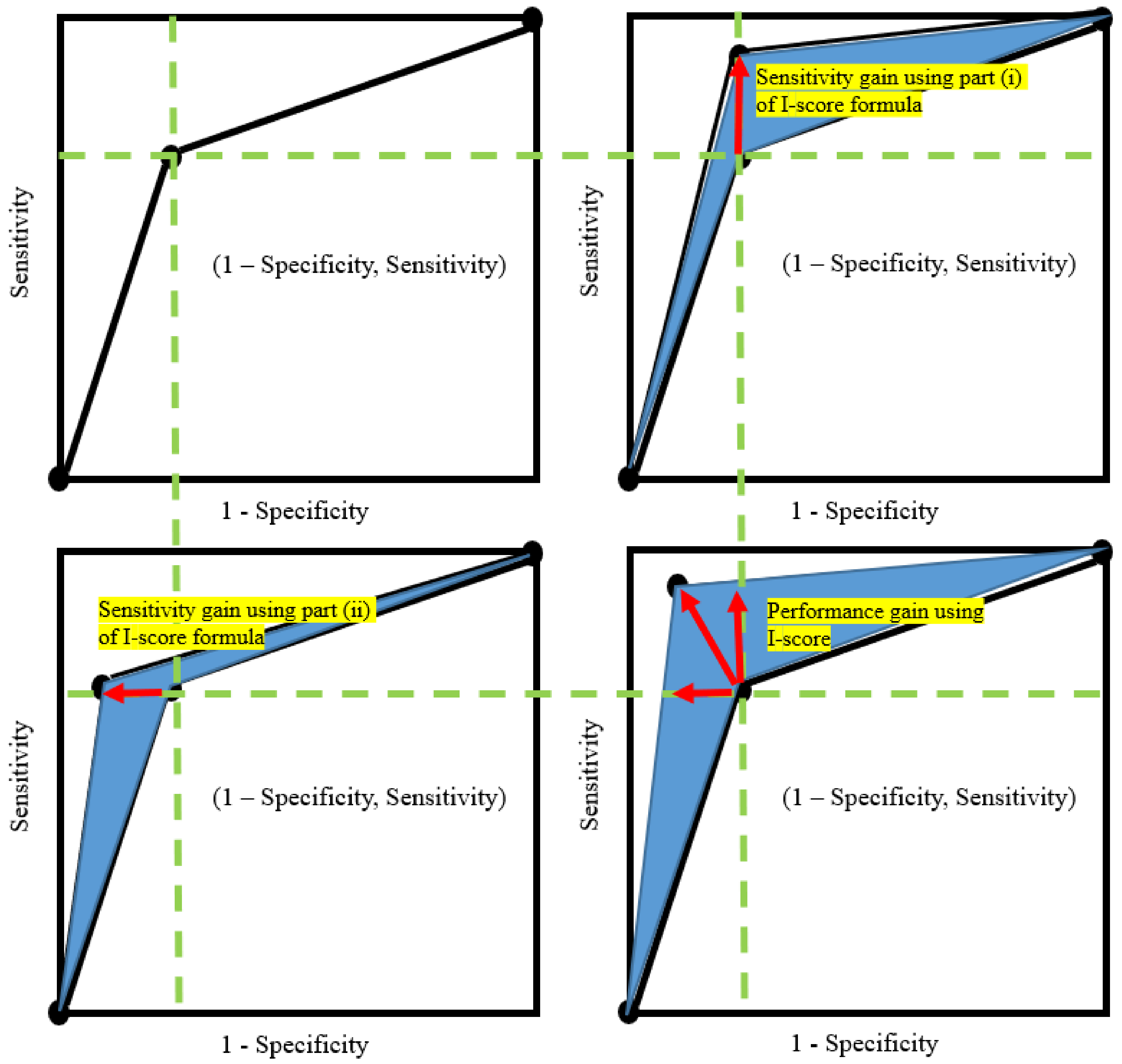
This means that if the variables with high sensitivity are selected, the I-score will increase, which corresponds to an increase in AUC. Alternatively, the nature of the I-score dictates to select highly-predictive variables with high sensitivity, which directly cause the ROC to move towards the top left corner of the plot (see Figure 1), i.e., resulting in higher AUC values.
Next, the second partition can be written as
Notice that under the scenario when the predictor is extremely informative, there can be very few observations for false negatives (which is ). In other words, when extremely predictive variables are present. In this case, the value of the second partition is completely determined by , which is largely dictated by the global average of the response variable Y but scaled up with a factor of . A benefit from a near-zero also implies that specificity can be high, which is another direction to push the AUC higher.
As a summary, the two partitions that consist of the main body of the I-score can be written as the following
where it allows us to conclude:
- First, part (i) is a function of sensitivity. More importantly, the I-score serves as a lower bound of sensitivity. The proposed statistics I-score is high when the sensitivity is high, which means the I-score can be used as a metric to select high sensitivity variables. A nice benefit from this phenomenon is that high sensitivity is the most important driving force to raise AUC values. This relationship is presented in the top right plot in Figure 1.
- Second, part (ii) is a function of , which approximates to zero value when the variable is highly predictive. This leaves the second part to be largely determined by the global average of the response variable Y but scaled up in proportion with the number of observations that fall in the second partition (), which is the sum . An interesting benefit from this phenomenon is that the near-zero value, jointly with part (i), implies that the specificity is high, which is another important driving force to raise AUC values. In other words, when the predictor has all the information to make a good prediction, the value of is expected to be approximately zero. In addition, the global mean of the true condition can be written as . Hence, this means that part (ii) can be rewritten as , where positively affect specificity because specificity is . Thus, part (ii) is a function of specificity.
- Third, the I-score is capable of measuring the variable set as a whole without making any assumption of the underlying model. However, AUC is defined between a response variable Y and a predictor . If a variable set has more than one variable, some underlying assumptions of the model need to be made—we would need —in order to compute the AUC value.
Remark
In a generalized situation, the confusion table in Table 3 may have more than two partitions for the predicted condition. In any scenario that the table has three or more partitions, they can be written into two partitions using a threshold. For example, instead of positive or negative, there can be predicted conditions to take values of . In this case, any number can be taken excluding 1 and K as a threshold to reduce K levels back into 2 levels. Suppose “2” is used as a threshold; the partitions greater than 2 can be one partition, and the partitions less than or equal to 2 can be one partition. This allows K levels to be reduced to 2 levels. The same proof in Equation (14) would follow.
2.2. An Interaction-Based Feature: Dagger Technique
The concept of an interaction-based feature was initially proposed by Lo and Yin (2021) [24]. In their work, the authors defined an interaction-based feature that is used to replace the construction of using filters in designing Convolutional Neural Networks (CNNs). The conventional practice relies on pre-defined filters, and these filters are small 2-by-2 or 3-by-3 windows that are designed to capture certain information based on prior knowledge. The art of using an interaction-based feature to create novel features within a 2-by-2 or 3-by-3 window in an image is to allow the data rather than meaningless filters to indicate the predictive information in the image. These new features are denoted as ’s, and hence the name “dagger technique”. The rest of this subsection formally defines this method of using partitions to define novel features.
A major benefit of using the proposed I-score is the partition-retention technique. This is a feature engineering technique that helps us to preserve the information of a variable set and convert it into one feature. Since ROC AUC cannot be directly computed between a response variable and the potential variable set, common procedure tends to fit a model first before AUC is computed. This is a very costly method for the following two reasons. First, the fitting of a regression or a classification model can be very costly to train. Second, the model fitting procedure cannot guarantee the prediction results of the final predictor. If the AUC value is low, there is no solution to distinguish whether the poor AUC result comes from model fitting or variable selection. The ROC curve and the computation of its AUC are only partially meaningful. Alternatively to the conventional AUC, partial AUC and the area under the precision-recall curve has been proposed [27]. However, the partial AUC cannot be interpreted as fully as the AUC because the method of partial AUC ignores some information about true negatives [27]. In this paper, it is shown with evidence in simulation that there can be extremely poor AUC values when the correct features are present with an incorrect estimation of the model (see Section 2.5 for simulation discussion and Table 4 for simulation results). We consider this the major drawback of using ROC AUC.
To tackle this problem, a proposed technique is to use partition retention. These new features are denoted as ’s, and hence this method is named the “dagger technique”. Now we introduce this technique as follows. Suppose there is a supervised learning problem and there is an explanatory variable X and response variable Y. Suppose X has a partition size k. A novel non-parametric feature can be created using the following formula
where k is the size of the total partitions formed by X. For example, suppose there is and . Then the variable set has four partitions, i.e., computed using . In this case, the running index for notating the partition j can take values . Then, based on this variable set , a new feature can be created called that is a combination of and using partition retention. Hence, this new feature can be defined as while , as discussed above. The results of this example is summarized in tabular form (see Table 2).
2.3. Discretization
The partition retention technique requires the partition space of the subset of variables in I-score formulation to be countable. In other words, the partition is necessary to form, and it can be defined by the subset disregarding how many variables are selected in this group b. If each variable takes values , then we have partitions for this subset . This is, however, not always guaranteed from practice. In some situations, there can be variables with many unique values that can be considered continuous. To avoid the sparsity problem (The sparsity problem arises when there are too many unique levels with lack of training sample size in the data. Without proper discretization or grouping techniques, we would have a partition with zero observations in it, which can slow down the computation of the statistics I-score.), we would need to discretize the continuous variable into a discrete variable. The algorithm is presented in Algorithm 1.
| Algorithm 1:Discretization. Procedure of Discretization for an Explanatory Variable |
 |
Suppose any explanatory variable has l unique levels while j in . That means we can use order statistics to write out all the unique levels using . To discrete from l levels into two levels, we need to choose a cutoff to compare all levels against this threshold (call it t), i.e., binary output based on t would be , in order to create a new variable that takes only values in . This threshold t can take any value in the unique levels, i.e., and at each t, we can compute the I-score using Equation (2). The best threshold would be the candidate that maximizes the I-score. The objective function can be stated as the following
while is dependent on the threshold t and can take , the partition is constructed based on an indicator function, i.e., , and can only be two partitions.
2.4. Backward Dropping Algorithm
In many situations, a variable set has noisy information that can damage the prediction performance. In this case, we recommend the Backward Dropping Algorithm to omit the noisy variables before we use machine learning or the “dagger technique”, which refers to the feature engineering technique in Equation (15).
The Backward Dropping Algorithm is a greedy algorithm to search for the optimal subsets of variables that maximize the I-score through step-wise elimination of variables from an initial subset sampled in some way from the variable space. The steps of the algorithm are as follows. Consider a training set of n observations, where is a p-dimensional vector of explanatory variables. The size p can be very large. All explanatory variables are discrete. Then we select an initial subset of k explanatory variables , . Next, we calculate . For the rest of the paper, we refer to this formula as the Influence Measure or Influence Score (I-score). Tentatively drop each variable in and recalculate the I-score with one variable less. Then drop the one that gives the highest I-score. Call this new subset , which has one variable less than . Continue to the next round of dropping variables in until only one variable is left. Keep the subset that yields the highest I-score in the entire process. Refer to this subset as the return set . This will be the most important and influential variable module from this initial training set. The above steps can be summarized in the following, see Algorithm 2.
| Algorithm 2:BDA. Procedure of the Backward Dropping Algorithm (BDA) |
 |
2.5. A Toy Example
Let us create the following simulation to further investigate the advantage the proposed I-score has over the conventional measure of AUC. In this experiment, suppose there are . In other words, the sequence of all 10 independent variables defined above can only take values from . We create a sample of 2000 observations for this experiment. Suppose we define the following model
while “mod” refers to a modulo of two, i.e., . We can compute the AUC values and the I-score values for all 10 variables. In addition, we also compute both measures for the following models (this is to assume when we do not know the true form of the real model): (i) , (ii) , (iii) , and (iv) . In model (iv), we add to ensure the division is legal. To further illustrate the power of the I-score statistic, we introduce a new variable specifically constructed by taking advantage of partition retention, i.e., , while (the novel dagger technique that is defined using a variable partition is widely used in application, see Equation (15)). The simulation has 2000 observations. We make a 50–50 split. The first 1000 observations are used to create partitions, and the local average of the target variable Y that is required in creating the feature is only taken from the first 1000 observations. In the next 1000 observations, we can directly observe and retain the partition. For each of the partitions, we then go to the training set (the first 1000 observations) and use the values created using only the training set. We present the simulation results in Table 4.
The simulation results show that the proposed I-score is capable of selecting truly predictive variables while the AUC values might be misleading. We can see that the challenge of this toy dataset is that the variables do not have a marginal signal. In other words, variables alone do not have predictive power. We can see this from the average AUC and I-score values. Since the AUC value cannot be computed using multiple variables directly, assumptions of the underlying models are built. We guess four models: (i) , (ii) , (iii) , and (iv) and these models all have low AUC values even though the variables are correct. This implies, under the false assumption of the underlying model, that AUC produces no reliable measure of detecting how significant the variables are. However, the proposed statistics on the assumed models (i)–(iv) are much higher than on individual variables alone. This means that the proposed I-score has the capability of detecting important variables even under incorrect assumptions of the model formulation.
The section “Guessed” in Table 4 consists of four assumed models containing the correct variables, , and the variable set . In this section, we observe that the AUC values are only high for and are rather poor in the rest of the assumed model. In addition, we cannot compute AUC for a variable set . Alternatively, we can use the I-score. The I-score values are drastically different in this section than the rest of the paper. The I-score for models (i) and (ii) are both above 700. The I-score for is exactly the same as the theoretical value, and so is the AUC for . This means the technique takes advantage of the partition of the variable set successfully and contains all the information that we need in order to make the best prediction result. This has not yet been discovered in the literature.
As a summary for this simulation, we can conclude the following
- In the scenario when the data set has many noisy variables and each variable observed does not have any marginal signal, the common practice AUC value will miss the information. This is because AUC still relies on the marginal signal. In addition, AUC is defined under the response variable Y and its predictor , which requires us to make assumptions on the underlying model formulation. This is problematic because the mistakes carried over in making the assumptions can largely affect the outcome of AUC. However, this challenge is not a roadblock for the proposed statistic I-score at all. In the same scenario with no marginal signal, as long as the important variables are involved in the selection, the I-score has no problem signaling us the high predictive power disregarding whether the correct form of the underlying model can be found or not.
- The proposed I-score is defined using the partition of the variable set. This variable set can have multiple variables in it, and the computation of the I-score does not require any assumption of the underlying model. This means the proposed I-score iss not subject to the mistakes carried over in the assumption or searching of the true model. Hence, the I-score is a non-parametric measure.
- The construction of the I-score can also be used to create a new variable that is based on the partition of any variable set. We call this new variable , hence the name “dagger technique”. It is an engineering technique that combines a variable set to form a new variable that contains all the predictive power that the entire variable set can provide. This is a very powerful technique due to its high flexibility. In addition, it can be constructed using the variables with a high I-score value after using the Backward Dropping Algorithm.
Table 4.
Simulation Results. This table presents the simulation results for the model . In this simulation, we create toy data with just 10 variables (all drawn from Bernoulli distribution with probability ). We define the true model using only the first two variables, and the remaining variables are noisy information. The task is to present the results of the AUC and the I-score values. The experiment is repeated 30 times, and we present the average and standard derivation (SD) of the AUC and I-score values. We can see that there is no marginal information contributed by any of the variables alone because each variable by itself has low AUC values and I-score values below 1 (if the I-score is below 1 it provides almost no predictive power). We can use the guessed model (i) to (iv) that is composed of the true variables (here we assume that we know is important, but we do not know the true form). We assign to ensure the division in model (iv) to be legal in the case . Last, we present the true model as a benchmark. Note: the “NA” entry means that AUC cannot be computed, i.e., not applicable or NA. The measure of AUC values has a major drawback: it cannot successfully detect useful information. Even with the correct variables selected (all guessed models only use the important variables ), AUC measures subjects to serious attack from incorrect model assumptions. This flaw renders applications of using the AUC measure to select models less ideal and sub-optimal. However, the proposed I-score is capable of indicating that the most important variables, and , disregard the forms of the underlying model. Moreover, the dagger technique of building using partitions generated by the variable set and completely recovers the full information of the true model even before any machine learning or model selection procedure, which is a novel invention that the literature has not yet seen.
| Average AUC | SD. of AUC | Average I-Score | SD. of I-Score | ||
|---|---|---|---|---|---|
| Important | 0.51 | 0.01 | 0.49 | 0.52 | |
| 0.51 | 0.01 | 0.52 | 0.68 | ||
| Noisy | 0.51 | 0.01 | 0.65 | 0.71 | |
| 0.5 | 0.01 | 0.41 | 0.6 | ||
| 0.51 | 0.01 | 0.61 | 0.77 | ||
| 0.5 | 0.01 | 0.27 | 0.29 | ||
| 0.51 | 0.01 | 0.42 | 0.7 | ||
| 0.5 | 0.01 | 0.33 | 0.48 | ||
| 0.51 | 0.01 | 0.49 | 0.68 | ||
| 0.51 | 0.01 | 0.39 | 0.48 | ||
| Guessed models (using ) | model (i): | 0.51 | 0.01 | 749.68 | 0.61 |
| model (ii): | 0.51 | 0.01 | 749.54 | 0.37 | |
| model (iii): | 0.49 | 0.25 | 248.2 | 18.26 | |
| model (iv): | 0.57 | 0.11 | 250.03 | 11.72 | |
| (see Equation (15)) | 1 | 0 | 999.14 | 0.54 | |
| NA | NA | 500.08 | 0.48 | ||
| True model | 1 | 0 | 999.14 | 0.54 |
2.6. Why I-Score?
2.6.1. Why Is I-Score the Best Candidate?
The design of the proposed I-score has the following three benefits. First, I-score is a non-parametric measurement. This means the I-score does not require any model fitting procedure. Second, the behavior of the I-score is parallel with that of AUC. If a predictor has a high I-score, this predictor must have a high AUC value. However, AUC cannot be directly defined if we have a set of variables. In this case, an estimation of the true model must be used in order to compute AUC, which means any attack from incorrect estimation of the true model will lower the AUC value. However, the I-score is not subject to this attack. Third, the proposed I-score can be developed into an interaction-based feature engineer method called the “dagger technique”. This technique can recover all useful information from a subset of variables. Next, we will explain each of the above three reasonings.
2.6.2. Non-Parametric Nature
The proposed I-score (Equation (2)) does not rely upon or make any assumptions on the model fitting procedure. The procedure of model fitting refers to the step of searching for a model that estimates the true relationship between features and the target variable. Suppose we have a subset of the features and their corresponding target variable Y. The relationship between and Y (denote this relationship to be ) is oftentimes not observable. We would have to make an assumption of the underlying model in order to construct a predictor . Only then can we measure the difference between our estimate and the true target variable. We can do so by using a loss function to estimate the error the predictor has at predicting the target variable Y. Disregarding the numerical magnitude of the result from the loss function, we are uncertain of the source of the mistakes we have. This is because the predictor is composed of both the estimation of the true model and the selected features . The literature has not yet discovered any procedure to directly measure the influence has on target variable Y without the estimation of the true model . Therefore, the error, measured by loss or ROC AUC values, is confounded, and we do not know clearly how the features influence the target variable Y, if it has any influence.
The proposed I-score can directly measure the influence features have on target variable Y without the usage of any estimation of the true model. In other words, the formula of the I-score (Equation (2)) has no component of , and there is no need to have as long as we can compute the I-score. This clears our judgment of feature selection and allows the end-users to immediately know not only the impact of the features but also how important they are in predicting the target variable Y.
From the toy example (see the simulation results in Table 4 in Section 2.5), we can see that the estimation of the true model, if incorrect, produces extremely poor AUC values (model (i)–(iv) in Table 4 have AUC values approximately 50%, equivalent to random guessing) even though the important and significant features are present in the variable set. The I-score is not subject to the attack of incorrect estimation of the true model. We can see that the I-score of the same incorrect models is extremely high, as long as the important features, , are included and present. Consequently, we regard this as the most important contribution and the reason why the I-score and the “dagger technique” are the best tools.
2.6.3. High I-Score Produces High AUC Values
We provide, in Section 2.1, a technical analysis on why a high I-score induces high AUC values. In the anatomy of the I-score formula in Section 2.1, we can see that the first partition (this is the partition when is positive) is directly related to sensitivity. In addition, we reward this outcome with a factor of , where is the number of observations that falls in this partition, i.e., is positive. This construction raises the I-score significantly and proportionately to the number of true positive cases, which is a major component causing the AUC value to rise. Hence, the benefit of using an I-score is that it allows statisticians and computer scientists to immediately identify the features that can raise the AUC values. This parallel behavior allows the easy interpretation of I-score values for its end-users.
Researchers have pointed out that ROC treats sensitivity and specificity equally [11], which can cause a lack of interpretability in some areas of practice such that the diagnostic is focusing on true positives. Poor sensitivity could mean that the experiment is missing the positive cases. In other words, AUC can consider a test that increases sensitivity at low specificity superior to one that increases sensitivity at high specificity. It is recommended that better tests should reward sensitivity to avoid false positives [28]. The construction of the I-score directly rewards sensitivity proportionate to the number of observations classified as positive cases correctly, which allows the I-score to exponentially grow as the sample size in the training set increases. This allows the I-score to not only behave in parallel to AUC values but is capable of reflecting the sensitivity values proportionate to the sample size.
2.6.4. I-Score and the “Dagger Technique”
The “dagger technique” is the most innovative method ever introduced, based on the literature in developing the I-score [21,22,23,26]. The proposed “dagger technique” organically combines the raw information from each feature by using partition retention [21], which allows the final combined feature to enrich the prediction performance free of incorrect estimation of the true model. This nature of the “dagger technique” is reflected in Table 4. The guessed models are all formulated using the correct variable sets: . However, model (i)–(iv) produced shocking 50% AUC values because AUC is subject to the attack of incorrect model estimation. This is a major drawback of using AUC to conduct model selection. However, the “dagger technique”, as long as the variable set includes the important variables, produces an outstanding 100% AUC with no variation. This means the “dagger technique” is capable of reconstructing the original information and enriching the predictor. We can see that the remaining methods all have some standard deviation when we simulate experiments with a different seed. However, the setting of different seeds has no impact on the proposed “dagger technique”, which means any time we use the “dagger technique”, we are able to recover the full information of the target variable Y with the correct variable set . This fact justifies the remarkable value of the “dagger technique” in the literature. The only other place that this is true in Table 4 is the model. Thus, the “dagger technique” has the capability to recover the full information from the target variable if the features are included correctly, and it is not subject to any attacks of false specification or estimation of the true model. We strongly recommend practitioners to use the proposed I-score and the “dagger technique” in the future whenever possible.
3. Application
3.1. Language Modeling
3.1.1. N-Gram
In Natural Language Processing, the prediction of the probability of a word or the classification of the label of a paragraph is a fundamental goal in building language models. The most basic language model is the “N-gram” model.
In “N-gram” modeling, a single word, such as “machine”, as a feature is a uni-gram (). The 2-word phrase “machine learning” is a bi-gram (). The 3-word phrase “natural language processing” is a tri-gram (). Any text document can be processed to construct N-gram features using this technique. For example, we may observe a sentence, and it states “I love this movie”. If the goal is to classify the sentence into one of the two classes: , a common practice is to estimate the probability of the label Y belongs to a certain class based on the previous words in the same sentence:
Joulin et al. (2016) [29] summarized a list of NLP algorithms to produce a range of performance from 80% to 90%. They also show evidence that N-gram models can increase the accuracy slightly more by using more N-grams. However, the aggregate N-gram models are not yet discovered. In addition, continuing adding N-gram features would result in overfitting, which leads to more and more complex architecture of RNN, such as Long Short Term Memory (LSTM), Gated Recurrent Unit (GRU), and bi-directional RNN. Thus far, there has not been any dimensionality reduction technique implemented within an RNN in the literature.
3.1.2. Recurrent Neural Network
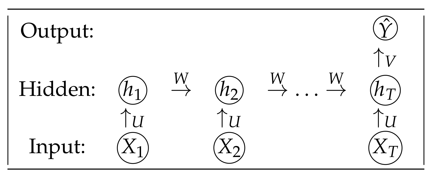
We introduced N-gram models above where the conditional probability of the label of a sentence y only depends on the previous words. Let us briefly discuss the basic RNN that we will use in the application. The diagram for the basic RNN is presented in Figure 2. Suppose we have input features . These features are directly processed from the text document, which can be processed by word index, or they can be embedded word vectors. The features are fed into the hidden layer where the neurons (or units) are denoted as . There is a weight connecting the previous neuron with the current neuron. We denote this weight as W. Each current neuron has a contribution from the current feature, which is connected with a weight parameter U. For any t in , we can compute each hidden neuron by using the following formula
where W and U are trainable parameters, b is the bias term, and can be an activation function. This choice of the activation function is completely determined by the dataset and the end-user. A list of famous activation functions can be found in Table 1. At the end of the architecture, we can finally compute the predicted probability of Y given the hidden neurons by using the formula
where the weights W, U, and V are shareable in the entire architecture. Forward propagation of RNN refers to the procedure when information flow from the input features to output predictor using Equations (19) and (20).
3.1.3. Backward Propagation Using Gradient Descent
The forward propagation allows us to pass information from the input layer, which are features extracted from text documents, to the output layer, which is the predictor. To search for the optimal weights, we need to compute the loss function and optimize the loss function by updating the weights. Since the task is text classification, we only have one output in the output layer. In addition, the task is a two-class classification problem because Y can only take the value of . This means we can define the loss function using the cross-entropy function, which is defined as
where is the true label for instance i and is the predicted value for instance i. Notice that in the proposed architecture we use the I-score and the “dagger technique” to construct for the input features where is smaller than T, and it is a length-dependent tuning process. Next, we can use gradient descent (GD) to update the parameters. At each step s, we can update the weights by
where is learning rate (usually a very small number), the symbol ∇ means gradient, and is the gradient (partial derivative) of the loss function . We can formally write the gradients in the following
where means gradient or partial derivative with respect to that parameter.
3.1.4. Implementation with I-Score
In this section, we introduce the proposed algorithm that is built upon the idea of a novel statistical measure I-score. The executive diagram for “N-gram” models using I-score as a feature selection and engineering technique is presented in Figure 3.
Figure 3 has presented two main pipelines for this paper that implements the proposed I-score into a basic RNN structure. Panel A presents the first simple framework of combining “N-grams” with I-score. The procedure of “N-grams” processes the text data into averaged numerical data. The conventional setup is presented in the left plot in Figure 2. The text document is processed using text vectorization, and then it is embedded into a matrix form. We can then fit a basic feed-forward ANN or sequential RNN. Panel B presents an alternative input using the “dagger technique”. We introduce them as follows.
The proposed I-score can be used in the following approaches:
- First, we can compute the I-score for each RNN unit. For example, in Figure 3A, we can first compute the I-score on the text vectorization layer. Then we can compute the I-score on the embedding layer. With the distribution of the I-score provided from the feature matrix, we can use a particular threshold to identify the cutoff used to screen for important features that we need to feed into the RNN architecture. We denote this action by using , and it is defined as . For the input layer, each feature can be released or omitted according to its I-score values. That is, we use to determine whether this input feature is predictive and important enough to be fed into the RNN architecture. For the hidden layer, each hidden neuron can be released or omitted according to its I-score values. In other words, we can use to determine whether this hidden neuron is important enough to be inserted in the RNN architecture. If at certain t the input feature fails to meet the certain I-score threshold ( would fail if the I-score of is too low, then ), then this feature is not fed into the architecture and the next unit is defined, using Equation (19), as . This is the same for any hidden neuron as well. If a certain hidden neuron has the previously hidden neuron , it fails to meet the I-score criteria, then is defined as . Hence, this function acts as a gate to allow the information of the neuron to pass through according to a certain I-score threshold. If is zero, that means this input feature is not important at all and hence can be omitted by replacing it with a zero value. In other words, it is as if this feature never existed. In this case, there is no need to construct . We show later in Section 3 that important long-term dependencies that are associated with language semantics can be detected using this function because I-score has the power to omit noisy and redundant features in the RNN architecture. Since I-score is compared throughout the entire length of T, the long-term dependencies between features that are far apart can be captured using high I-score values.
- Second, we can use the “dagger technique” to engineer and craft novel features using Equation (15). We can then calculate the I-score on these dagger feature values to see how important they are. We can directly use a 2-gram model, and the I-score is capable of indicating which 2-gram phrases are important. These phrases can act as two-way interactions. According to the I-score, we can then determine whether we want all the words in the 2-gram models, 3-gram models, or even higher level of N-gram models. When n is large, we recommend using the proposed Backward Dropping Algorithm to reduce dimensions within the N-word phrase before creating a new feature using the proposed “dagger technique”. For example, suppose we use the 2-gram model. A sentence such as “I love my cats” can be processed into (I, love), (love, my), (my, cats). Each feature set has two words. We can denote the original sentence “I love my cats” into four features . The “dagger technique” suggests that we can use Equation (15) with 2-gram models fed in as inputs. In other words, we can take and construct , where j is the running index tracking the partitions formed using . If we discretize and (see Section 2.3 for a detailed discussion of discretization using the I-score) and they both take values of , then there are partitions, and hence j can take values of . In this case, the novel feature can take on four values, i.e., an example can be seen in Table 2. The combination of the I-score, Backward Dropping Algorithm, and the “dagger technique” allows us to prune the useful and predictive information in a feature set so that we can achieve maximum prediction power with as few features as possible.
- Third, we can concatenate many N-gram models with different n values. For example, we can carry out N-gram modeling using , , and . This way, we can combine more high-order interactions. In order to avoid overfitting, we can use the I-score to select the important interactions and then use these selected phrases (which can be two-word, three-word, or four-word) to build RNN models.
3.2. IMDB Dataset
In this application, we use the IMDB movie database, which includes 25,000 paragraphs in the training and testing sets. In total, there are 50,000 paragraphs, and each paragraph carries a label. The label is dichotomous, i.e., if the review is positive and if the review is negative. A sample of the data is presented in Table 5. The first sample is a positive review. The second sample is a negative review.
In the experiment of text classification, we use data provided in the IMDB movie database. The dataset consists of 25,000 observations in each of the training and testing sets. In total, there are 50,000 observations. The dataset has equal portions for two classes. The two classes are if the movie review is positive and if the movie review is negative. The goal is to read a paragraph and predict whether the tone of this paragraph of the movie review is positive or negative. We present sample data in Table 5.
Table 5.
Sample Data and Selected Semantics. This table presents sample data. We present two samples. The first column is the paragraphs directly taken from the IMDB movie database. The second column is the corresponding label for the first column. The proposed I-score selects words that have a significant association with the semantics of the sentence. This is because I-score selects features that are highly predictive of the target variable. In this application, the target variable carries tones and preferences of a movie of which the same writer provides critics and reviews. The semantics in the critics and reviews reflect the tones and the preferences of the movie reviewers, which is why the I-score is able to detect the features using the provided preferences in the label.
| No. | Samples | I-Score Features | Label | |
|---|---|---|---|---|
| Uni–Gram | 2-Gram, 3-Gram | |||
| 1 | this film was just brilliant casting location scenery story direction everyone’s really suited the part they played and you could just imagine being there robert is an amazing actor and now the same being director father came from the same scottish island as myself so i loved the fact there was a real connection with this film the witty remarks throughout the film were great it was just brilliant so much that i bought the film as soon as it was released for retail and … | {congratulations, lovely, true} | {amazing actor, really suited} | 1 |
| 2 | big hair big boobs bad music and a giant safety pin these are the words to best describe this terrible movie i love cheesy horror movies and i’ve seen hundreds but this had got to be on of the worst ever made the plot is paper thin and ridiculous the acting is an abomination the script is completely laughable the best is the end showdown with the cop and how he worked out who the killer is it’s just so damn terribly written … | {bad, ridiculous} | {bad music, terribly written}, {damn terribly written} | 0 |
In Table 5, we present evidence that the I-score can detect important words that are highly impactful for predicting the label of positive or negative tones. In Table 6, we present the semantics of the same two samples that the I-score narrows down. The original RNN uses the processed word vector to make predictions. For example, scholars have been using N-gram models to extract features from the text document [29]. Other common techniques of feature extractions are Term Frequency-Inverse Document Frequency (TF-IDF), Term Frequency (TF) [30], Word2Vec [31], and Global Vectors for Word Representation (GloVe) [32]. However, I-score is able to shrink the word counts with the reduced dimensions to be a tuning parameter. In this experiment, we reduce the number of words from 400 to 100 or even 30 while keeping the same semantics. This dimension reduction technique is completely novel and can provide what goes beyond human intuition in language semantics problems in NLP.
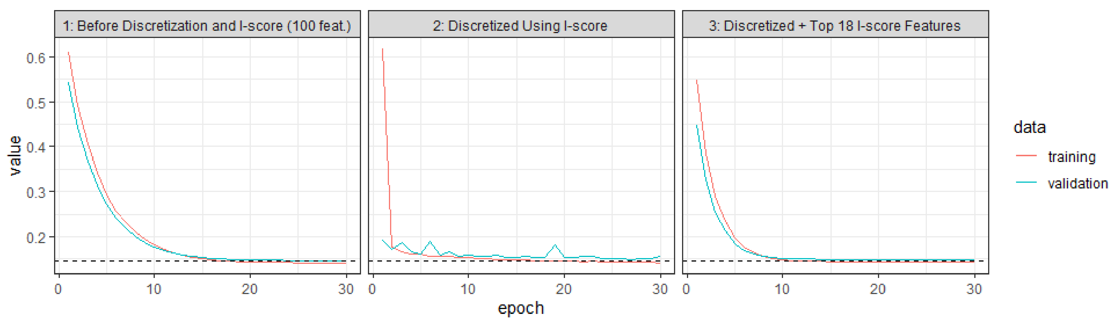
The training and validating process is summarized in Table 4. In Figure 4, we summarize the training and the validating paths that are generated from the experiment before and after using the proposed statistics I-score. The first plot of Figure 4 presents the training and validating paths for the original bi-gram data (here the data are processed into 100 features). The second plot of Figure 4 is the same data but discretized using I-score.
Table 6.
Interpreted Semantics Using I-score. This table presents sample data. We present two samples. The first column is the paragraphs directly taken from the IMDB movie database. The second column presents features selected by I-score according to different I-score thresholds (we use the top 7.5% and the top 25% as examples). The last column presents the corresponding label. The semantics of the selected features are a subset of words from the original sample. We observe that I-score can select a subset of words while maintaining the same semantics.
| No. | Samples (Original Paragraphs) | I-Score Features (Using Different Thresholds) | Label | |
|---|---|---|---|---|
| Top 7.5% I-Score | Top 25% I-Score | |||
| 1 | this film was just brilliant casting location scenery story direction everyone’s really suited the part they played and you could just imagine being there robert is an amazing actor and now the same being director father came from the same scottish island as myself so i loved the fact there was a real connection with this film the witty remarks throughout the film were great it was just brilliant so much that i bought the film as soon as it was released for retail and would recommend it to everyone to watch and the fly fishing was amazing really cried at the end it was so sad and you know what they say if you cry at a film it must have been good and this definitely was also congratulations to the two little boy’s that played the of … | {congratulations often the play them all a are and should have done you think the lovely because it was true and someone’s life after all that was shared with us all} | {for it really at the so sad you what they at a must good this was also congratulations to two little boy’s that played the <UNK> of norman and paul they were just brilliant children are often left out the praising list i think because the stars that play them all grown up are such a big profile for the whole film but these children are amazing and should be praised for what they have done do not you think the whole story was so lovely because it was true and was someone’s life after all that was shared with us all} | 1 |
| 400 words | 31 words | 101 words | ||
| 2 | big hair big boobs bad music and a giant safety pin these are the words to best describe this terrible movie i love cheesy horror movies and i’ve seen hundreds but this had got to be on of the worst ever made the plot is paper thin and ridiculous the acting is an abomination the script is completely laughable the best is the end showdown with the cop and how he worked out who the killer is it’s just so damn terribly written the clothes are sickening and funny in equal measures the hair is big lots of boobs bounce men wear those cut tee shirts that show off their sickening that men actually wore them and the music is just trash that plays over and over again in almost every scene there is trashy music boobs and … | {those every is trashy music away all aside this whose only is to look that was the 80’s and have good old laugh at how bad everything was back then} | {script best worked who the just so terribly the clothes in equal hair lots boobs men wear those cut shirts that show off their sickening that men actually wore them and the music is just trash that over and over again in almost every scene there is trashy music boobs and taking away bodies and the gym still does not close for all joking aside this is a truly bad film whose only charm is to look back on the disaster that was the 80’s and have a good old laugh at how bad everything was back then} | 0 |
| 400 words | 31 words | 101 words | ||
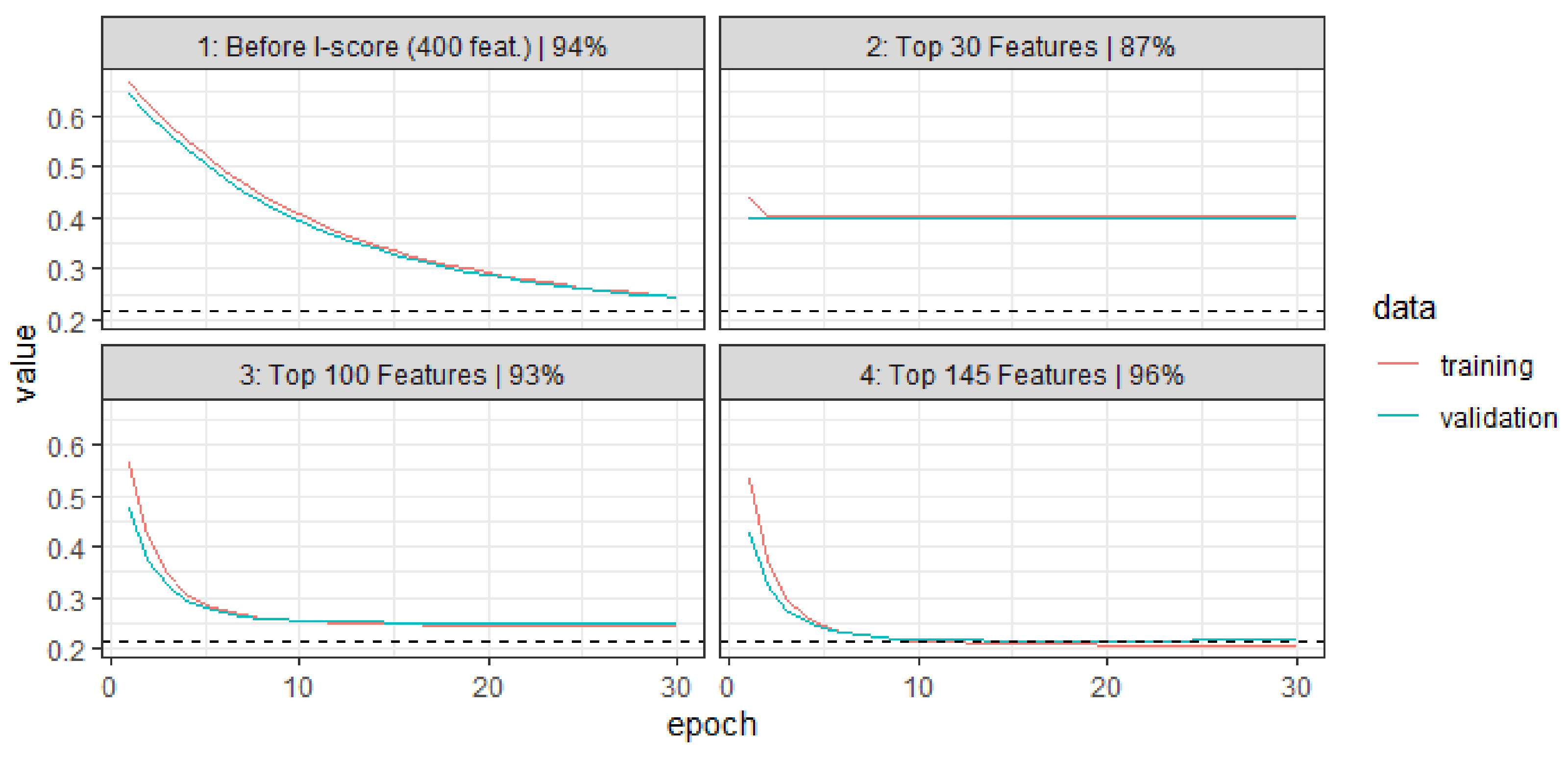
Figure 5 presents the learning paths before and after dimensionality reduction using the proposed I-score. To demonstrate the potential of the I-score, we first use the extracted features from the embedding layer, which generates 400 features (a tuning result). We can use these 400 features to send into a feed-forward ANN or sequential RNN. The test set performance is 94%, which is measured using AUC values. We can compute marginal I-scores (this means we compute the I-score using each variable as a predictor independently). Amongst these 400 features, we can rank them using I-score values and pick the top 30 features. We feed these 30 features into a feed-forward ANN or sequential RNN, and we have already achieved 87% on the test set. To further improve the learning performance, we can increase the I-score threshold so that we can include more top influential features. We can use the top 30, 100, and 145, respectively. We plot the learning paths in Figure 5. The first graph “1”, is the learning path for the original 400 features. We can see that the training set and validating set error merely breached 0.2 in 30 epochs. However, when we use the top 100 features, we are able to see in graph “3” that we are able to achieve a near convergence of approximately 10 epochs. This increased convergence speed is largely due to the nature that I-score is able to erase the noisy and redundant features from the input layer. In addition, the I-score is able to deliver this efficient learning performance with only 25% of the number of the original features, which is something the literature has not yet seen. We regard this as another major benefit of using the proposed technique in training neural networks.
3.3. Results
We show in Table 7 the experiment results for the text classification task in the IMDB Movie Dataset. We start with bi-gram models. The performance of using I-score to select the important bi-gram features produced 96.5% AUC on the test set while the bi-gram model without I-score produced 92.2%. We also used a combination of different N-gram models while we set the level of N to be , i.e., 2-gram, 3-gram, and 4-gram, respectively. We can concatenate the N-gram features and then feed the features into a feed-forward neural network directly. First, we concatenate the 2-gram and 3-gram models together and then we use I-score to reduce the prediction performance. We recommend using the top 5% I-score threshold to screen for the important semantics among all the 2-gram and 3-gram features. This corresponds to approximately 40 out of the 800 concatenated 2-gram and 3-gram features. We observe that the I-score is able to raise the prediction performance to 97.7% while a combination of 2-gram and 3-gram model without the I-score is only able to produce 91.1%, which is a 74% error reduction.
Remark 1.
Though this paper investigates the IMDB Movie Dataset (a relatively well-known data set), the proposed methods’ I-score, Backward Dropping Algorithm, and the Dagger Technique have been adapted in other data sets, such as Chest X-ray Images (both binary classes and 4-class classifications), to produce the state-of-the-art results at 99.7% AUC on the held-out test set while using only 12,000–15,000 trainable parameters in the proposed neural network architecture, which is almost a 98% reduction in the number of trainable weights comparing with peers [24,25].
Table 7.
Test Performance Comparison. The table presents experimental results of prediction performance on the IMDB dataset. The performance is measured in AUC, and the proposed method increases the prediction result to 97%, which is an 85% error reduction.
Table 7.
Test Performance Comparison. The table presents experimental results of prediction performance on the IMDB dataset. The performance is measured in AUC, and the proposed method increases the prediction result to 97%, which is an 85% error reduction.
| Model | IMDB (Test Set) |
|---|---|
| CNN [33] | 37.5% |
| RNN | 85.7% |
| LSTM | 86.6% |
| GRU | 86.7% |
| 2-gram | 92.2% |
| 2-gram + 3-gram | 91.1% |
| 2-gram + 3-gram + 4-gram | 90.2% |
| Average: | 81% |
| Proposed: | |
| 2-gram: use high I-score features | 96.5% |
| 2-gram + 3-gram: use high I-score features | 96.7% |
| 2-gram + 3-gram + 4-gram: use high I-score features | 97.2% |
| 2-gram + 3-gram + 4-gram: use novel “dagger” features (based on Equation (15)) | 97.2% |
4. Conclusions
This paper proposes a novel I-score to detect and search for the important language semantics in text documents that are useful for making good predictions in text classification tasks.
Theoretical Contribution. We provide theoretical and mathematical reasoning as to why I-score can be considered a function of AUC. The construction of the I-score can be analyzed using partitions. We see from mathematical rearrangements of the I-score formula that sensitivity plays a major component. This role of I-score provides the fundamental driving force to raise AUC values if the variables selected to compute I-score are important and significant. In addition to its theoretical parallelism with AUC, I-score can be used anywhere in a neural network architecture, which allows its end-users to flexibly deploy this computation, which is a feature that does not exist in AUC. AUC is also vulnerable under incorrect model specifications. Any estimation of the true model, disregarding whether it is accurate or not, is harmless to the performance of the I-score due to its non-parametric nature, which is a novel measure for feature selection that the literature has not yet seen.
Backward Dropping Algorithm. We also propose a greedy search algorithm called the Backward Dropping Algorithm that handles long-term dependencies in the dataset. Under the curse of dimensionality, the Backward Dropping Algorithm is capable of efficiently screening out the noisy and redundant information. The design of the Backward Dropping Algorithm also takes advantage of the nature of the I-score, because the I-score increases when the variable set has less noisy features, while the I-score decreases when the noisy features are included.
Dagger Technique. We propose a novel engineering technique called the “dagger technique” that combines a set of features using partition retention to form a new feature that fully preserves the relationship between the explanatory variable and the response variable. This proposed “dagger technique” can successfully combine words and phrases with long-term dependencies into one new feature that carries long-term memory. It can also be used in constructing the features in many other types of deep neural networks, such as Convolutional Neural Networks (CNNs). Though we present empirical evidence in sequential data application, this “dagger technique” can actually go beyond most image data and sequential data.
Application. We show, with empirical results, that this “dagger technique” can fully reconstruct target variables with the correct features, which is a method that can be generalized into any feed-forward Artificial Neural Network (ANN) and Convolutional Neural Network (CNN). We demonstrate the usage of I-score and the proposed methods with simulation data. We also show with a real-world application on the IMDB Movie dataset that the proposed methods can achieve 97% AUC value, an 81% error reduction from its peers or similar RNNs without an I-score.
Future Research Directions. We call for further exploration in the direction of using the I-score to extrapolate features that have long-term dependencies in time-series and sequential data. Since it is computationally costly to rely on high-performance CPU/GPUs, the direction I-score is taking leads researchers to rethink designing longer and deeper neural networks. Instead, future research can continue under the approach of building low dimensional but extremely informative features so that we can construct less complicated models in order for end-users.
Author Contributions
Conceptualization, S.-H.L. and Y.Y.; methodology, S.-H.L. and Y.Y.; software, Y.Y.; formal analysis: S.-H.L. and Y.Y.; validation, Y.Y.; writing—original, review and editing, S.-H.L. and Y.Y. All authors have read and agreed to the published version of the manuscript.
Funding
This research is supported by the National Science Foundation BIGDATA IIS 1741191.
Institutional Review Board Statement
Not applicable.
Informed Consent Statement
Not applicable.
Data Availability Statement
Data is contained within the article.
Acknowledgments
We would like to dedicate this to H. Chernoff, a well-known statistician and a mathematician worldwide, in honor of their 98th birthday and their contributions to Influence Score (I-score) and the Backward Dropping Algorithm (BDA). We are particularly fortunate in receiving many useful comments from him. Moreover, we are very grateful for their guidance on how I-score plays a fundamental role that measures the potential ability to use a small group of explanatory variables for classification, which leads to much broader impacts in fields of pattern recognition, computer vision, and representation learning.
Conflicts of Interest
The authors declare no conflict of interest.
References
- Salehinejad, H.; Sankar, S.; Barfett, J.; Colak, E.; Valaee, S. Recent advances in recurrent neural networks. arXiv 2017, arXiv:1801.01078. [Google Scholar]
- Bengio, Y.; Boulanger-Lewandowski, N.; Pascanu, R. Advances in optimizing recurrent networks. In Proceedings of the 2013 IEEE International Conference on Acoustics, Speech and Signal Processing, Vancouver, BC, Canada, 26–31 May 2013; pp. 8624–8628. [Google Scholar]
- Hinton, G.E.; Osindero, S.; Teh, Y.W. A fast learning algorithm for deep belief nets. Neural Comput. 2006, 18, 1527–1554. [Google Scholar] [CrossRef] [PubMed]
- Mahmood, M.A.; Popescu, A.C.; Oane, M.; Channa, A.; Mihai, S.; Ristoscu, C.; Mihailescu, I.N. Bridging the analytical and artificial neural network models for keyhole formation with experimental verification in laser-melting deposition: A novel approach. Results Phys. 2021, 26, 104440. [Google Scholar] [CrossRef]
- Mahmood, M.A.; Visan, A.I.; Ristoscu, C.; Mihailescu, I.N. Artificial neural network algorithms for 3d printing. Materials 2021, 14, 163. [Google Scholar] [CrossRef]
- Bengio, Y.; Simard, P.; Frasconi, P. Learning long-term dependencies with gradient descent is difficult. IEEE Trans. Neural Networks 1994, 5, 157–166. [Google Scholar] [CrossRef]
- Sutskever, I.; Martens, J.; Hinton, G.E. Generating text with recurrent neural networks. In Proceedings of the 28th International Conference on Machine Learning, ICML 2011, Bellevue, WA, USA, 28 June–2 July 2011. [Google Scholar]
- Kowsari, K.; Jafari Meimandi, K.; Heidarysafa, M.; Mendu, S.; Barnes, L.; Brown, D. Text classification algorithms: A survey. Information 2019, 10, 150. [Google Scholar] [CrossRef] [Green Version]
- Spirovski, K.; Stevanoska, E.; Kulakov, A.; Popeska, Z.; Velinov, G. Comparison of different model’s performances in task of document classification. In Proceedings of the 8th International Conference on Web Intelligence, Mining and Semantics, Novi Sad, Serbia, 25–27 June 2018; pp. 1–12. [Google Scholar]
- Jayawant, N. Mandrekar. Receiver operating characteristic curve in diagnostic test assessment. J. Thorac. Oncol. 2010, 5, 1315–1316. [Google Scholar]
- Halligan, S.; Altman, D.G.; Mallett, S. Disadvantages of using the area under the receiver operating characteristic curve to assess imaging tests: A discussion and proposal for an alternative approach. Eur. Radiol. 2015, 25, 932–939. [Google Scholar] [CrossRef] [Green Version]
- Apicella, A.; Donnarumma, F.; Isgrò, F.; Prevete, R. A survey on modern trainable activation functions. Neural Netw. 2021, 138, 14–32. [Google Scholar] [CrossRef]
- Bengio, Y.; LeCun, Y. Scaling learning algorithms towards ai. Large-Scale Kernel Mach. 2007, 34, 1–41. [Google Scholar]
- Girshick, R.; Donahue, J.; Darrell, T.; Malik, J. Rich feature hierarchies for accurate object detection and semantic segmentation. In Proceedings of the IEEE Conference on Computer Vision and Pattern Recognition, Columbus, OH, USA, 23–28 June 2014; pp. 580–587. [Google Scholar]
- Guyon, I.; Weston, J.; Barnhill, S.; Vapnik, V. Gene selection for cancer classification using support vector machine. Mach. Learn. 2002, 46, 389–422. [Google Scholar] [CrossRef]
- He, K.; Zhang, X.; Ren, S.; Sun, J. Deep residual learning for image recognition. In Proceedings of the IEEE Conference on Computer Vision and Pattern Recognition, Las Vegas, NV, USA, 27–30 June 2016; pp. 770–778. [Google Scholar]
- Huang, G.; Liu, Z.; Van Der Maaten, L.; Weinberger, K.Q. Densely connected convolutional networks. In Proceedings of the IEEE Conference on Computer Vision and Pattern Recognition, Las Vegas, NV, USA, 27–30 June 2017. [Google Scholar]
- Krizhevsky, A.; Sutskever, I.; Hinton, G.E. Imagenet classification with deep convolutional neural networks. Adv. Neural Inf. Process. Syst. 2012, 25, 1097–1105. [Google Scholar] [CrossRef]
- LeCun, Y.; Boser, B.; Denker, J.S.; Henderson, D.; Howard, R.E.; Hubbard, W.; Jackel, L.D. Handwritten digit recognition with a back-propagation network. Adv. Neural Inf. Process. Syst. 1989, 2, 396–404. [Google Scholar]
- LeCun, Y.; Bengio, Y.; Hinton, G. Deep learning. Nature 2015, 521, 436–444. [Google Scholar] [CrossRef]
- Chernoff, H.; Lo, S.H.; Zheng, T. Discovering influential variables: A method of partitions. Ann. Appl. Stat. 2009, 3, 1335–1369. [Google Scholar] [CrossRef] [Green Version]
- Lo, A.; Chernoff, H.; Zheng, T.; Lo, S.H. Why significant variables aren’t automatically good predictors. Proc. Natl. Acad. Sci. USA 2015, 112, 13892–13897. [Google Scholar] [CrossRef] [Green Version]
- Lo, A.; Chernoff, H.; Zheng, T.; Lo, S.H. Framework for making better predictions by directly estimating variables’ predictivity. Proc. Natl. Acad. Sci. USA 2016, 113, 14277–14282. [Google Scholar] [CrossRef] [Green Version]
- Lo, S.H.; Yin, Y. An interaction-based convolutional neural network (icnn) towards better understanding of COVID-19 x-ray images. arXiv 2021, arXiv:2106.06911. [Google Scholar]
- Lo, S.H.; Yin, Y. A novel interaction-based methodology towards explainable ai with better understanding of pneumonia chest x-ray images. arXiv 2021, arXiv:2104.12672. [Google Scholar]
- Lo, S.H.; Zheng, T. Backward haplotype transmission association algorithm—A fast multiple-marker screening method. Hum. Hered. 2002, 53, 197–215. [Google Scholar] [CrossRef] [Green Version]
- Carrington, A.M.; Fieguth, P.W.; Qazi, H.; Holzinger, A.; Chen, H.H.; Mayr, F.; Manuel, D.G. A new concordant partial auc and partial c statistic for imbalanced data in the evaluation of machine learning algorithms. BMC Med. Inform. Decis. Mak. 2020, 20, 4. [Google Scholar] [CrossRef] [PubMed]
- Baker, S.G. The central role of receiver operating characteristic (roc) curves in evaluating tests for the early detection of cancer. J. Natl. Cancer Inst. 2003, 95, 511–515. [Google Scholar] [CrossRef] [PubMed] [Green Version]
- Joulin, A.; Grave, E.; Bojanowski, P.; Mikolov, T. Bag of tricks for efficient text classification. arXiv 2016, arXiv:1607.01759. [Google Scholar]
- Salton, G.; Buckley, C. Term-weighting approaches in automatic text retrieval. Inf. Process. Manag. 1988, 24, 513–523. [Google Scholar] [CrossRef] [Green Version]
- Goldberg, Y.; Levy, O. word2vec explained: Deriving mikolov et al.’s negative-sampling word-embedding method. arXiv 2014, arXiv:1402.3722. [Google Scholar]
- Pennington, J.; Socher, R.; Manning, C.D. Glove: Global vectors for word representation. In Proceedings of the 2014 Conference on Empirical Methods in Natural Language Processing (EMNLP), Doha, Qatar, 25–29 October 2014; pp. 1532–1543. [Google Scholar]
- Tang, D.; Qin, B.; Feng, X.; Liu, T. Effective lstms for target-dependent sentiment classification. arXiv 2015, arXiv:1512.01100. [Google Scholar]
Figure 1.
Mechanism between I-score gain and AUC gain. This figure presents the mechanism of how the I-score can increase AUC. There are four plots. The top left plot is a ROC curve with one particular pair of (1-Specificity, Sensitivity). The top right plot presents sensitivity gain from the I-score. The bottom left plot presents specificity gain from the I-score. Both sensitivity and specificity are driving forces of the AUC values because they move the dot up or left, which then increases the area-under-curve (the blue area). The bottom right plot presents performance gain from both sensitivity and specificity. In summary, the implementation of using the proposed I-score can increase AUC by selecting the features raising both sensitivity (from part (i) of the I-score, see Equation (14)) and specificity (from part (ii) of the I-score, see Equation (14)).

Figure 2.
A Simple RNN for Text Classification. This diagram illustrates the basic steps of using RNN for text classification. The input features are . The hidden neurons are . The output prediction is . Since this is the text classification problem, the architecture has many inputs and one output, hence the name “many-to-one”. The architecture has parameters and these weights (or parameters) are shareable throughout the architecture.

Figure 3.
Executive Diagram for the Proposed Method. This figure represents the proposed methodologies using N-grams, I-score, and the “dagger technique”. The forward propagation and the backward propagation remain the same before and after using I-score. The function acts as a gate to release the neuron according to certain I-score criteria. (A) Panel A presents the Recurrent Neural Network design to implement I-score at each step of the neural network architecture. (B) Panel B presents features constructed using the “dagger technique” and then fed into the Recurrent Neural Network (RNNs) architecture.

Figure 4.
Learning Paths Before and After Discretization. This figure presents the training procedure. All graphs present the training and validating paths. The first graph is from the original bi-gram data. The second is from using discretized bi-gram (discretized by I-score). The third is using the top 18 variables according to I-score values. The proposed method can significantly improve the computation efficiency.

Figure 5.
Learning Paths Before and After Text Reduction Using I-score. This figure presents the training procedure. All graphs present the training and validating paths. The first graph is from the original bi-gram data. The second is from using discretized bi-gram (discretized by I-score). The third is using the top 18 variables according to I-score values. The proposed method can significantly improve the computation efficiency.

Table 1.
Famous Activation Functions. This table presents three famous non-linear activation functions used in a neural network architecture. We use the ReLU as the activation function in the hidden layers and the Sigmoid as the activation function for the output unit. The activation functions are discussed in detais in Apicella (2021) [12], and we also compute the derivatives of these common activations in the table.
| Name | Function | Figure | Derivative |
|---|---|---|---|
| Sigmoid |  | ||
| tanh |  | ||
| ReLU |  |
Table 2.
Interaction-based Engineer: “Dagger Technique”. This table summarizes the construction procedure of (the “dagger technique”). Suppose there is a variable set and each of them can take values in . The can be constructed, and the values of this new feature are defined using the local average of the target variable Y based on the partition retained from the variable set . Here the variable set produces four partitions. Therefore, the can be defined according to the following table. In the test set, the target variable (or response variable) Y is not observed, so the training set values are used. Hence, the reminder is that in generating test set , we use ’s from the training set.

Publisher’s Note: MDPI stays neutral with regard to jurisdictional claims in published maps and institutional affiliations. |
© 2021 by the authors. Licensee MDPI, Basel, Switzerland. This article is an open access article distributed under the terms and conditions of the Creative Commons Attribution (CC BY) license (https://creativecommons.org/licenses/by/4.0/).
Share and Cite
MDPI and ACS Style
Lo, S.-H.; Yin, Y. Language Semantics Interpretation with an Interaction-Based Recurrent Neural Network. Mach. Learn. Knowl. Extr. 2021, 3, 922-945. https://0-doi-org.brum.beds.ac.uk/10.3390/make3040046
AMA Style
Lo S-H, Yin Y. Language Semantics Interpretation with an Interaction-Based Recurrent Neural Network. Machine Learning and Knowledge Extraction. 2021; 3(4):922-945. https://0-doi-org.brum.beds.ac.uk/10.3390/make3040046
Chicago/Turabian StyleLo, Shaw-Hwa, and Yiqiao Yin. 2021. "Language Semantics Interpretation with an Interaction-Based Recurrent Neural Network" Machine Learning and Knowledge Extraction 3, no. 4: 922-945. https://0-doi-org.brum.beds.ac.uk/10.3390/make3040046