Holocene Hydroclimate Variability in Central Scandinavia Inferred from Flood Layers in Contourite Drift Deposits in Lake Storsjön

 ,
,
Abstract
:1. Introduction
2. Materials and Methods
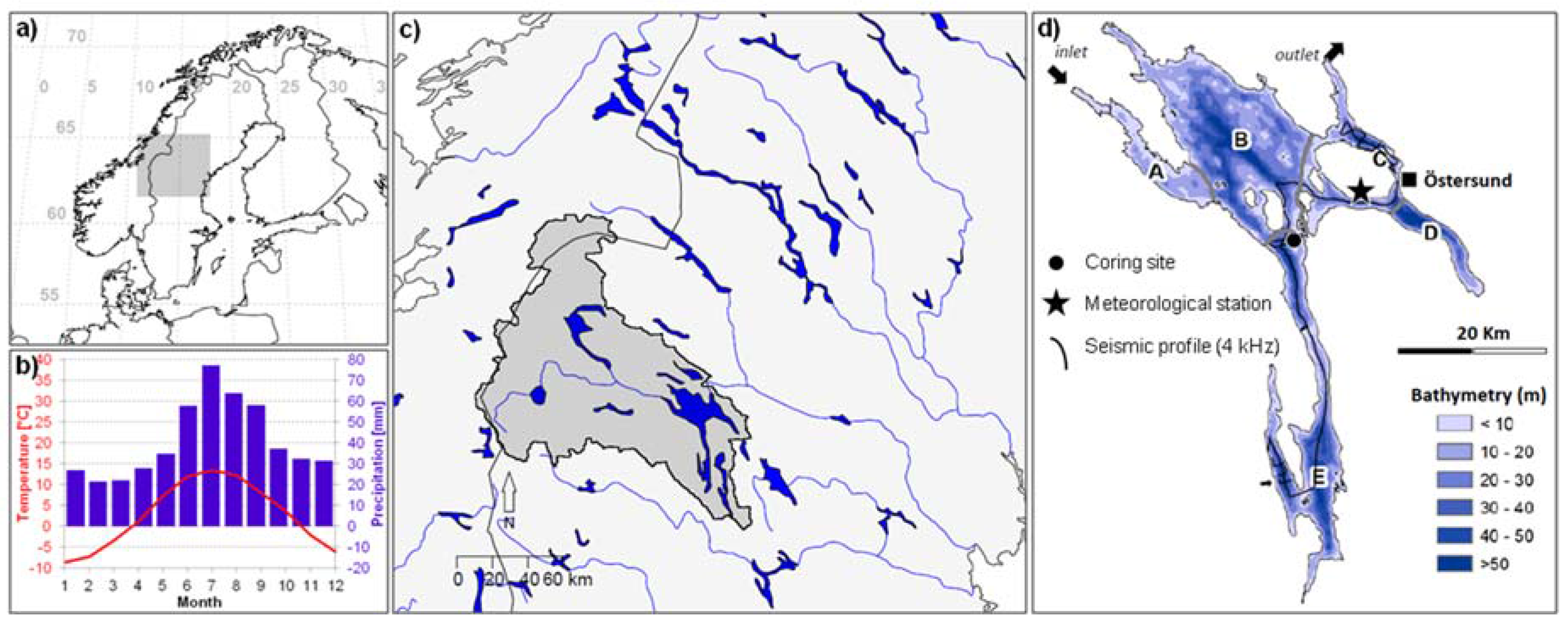
2.1. Study Area
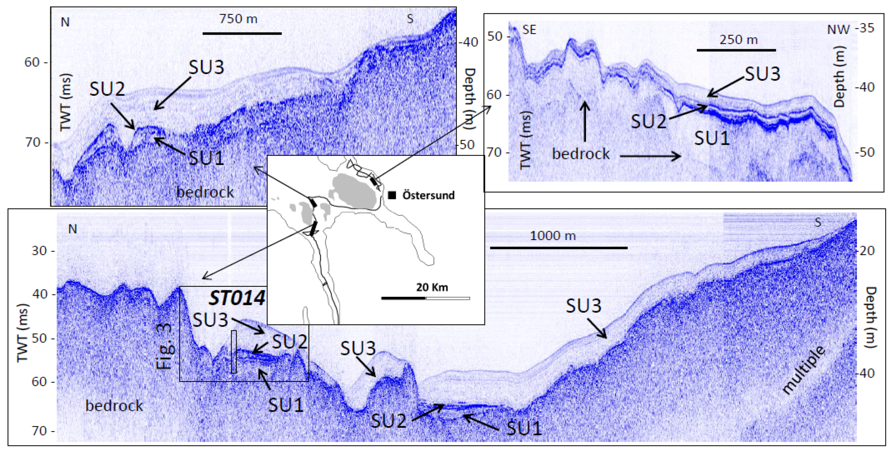
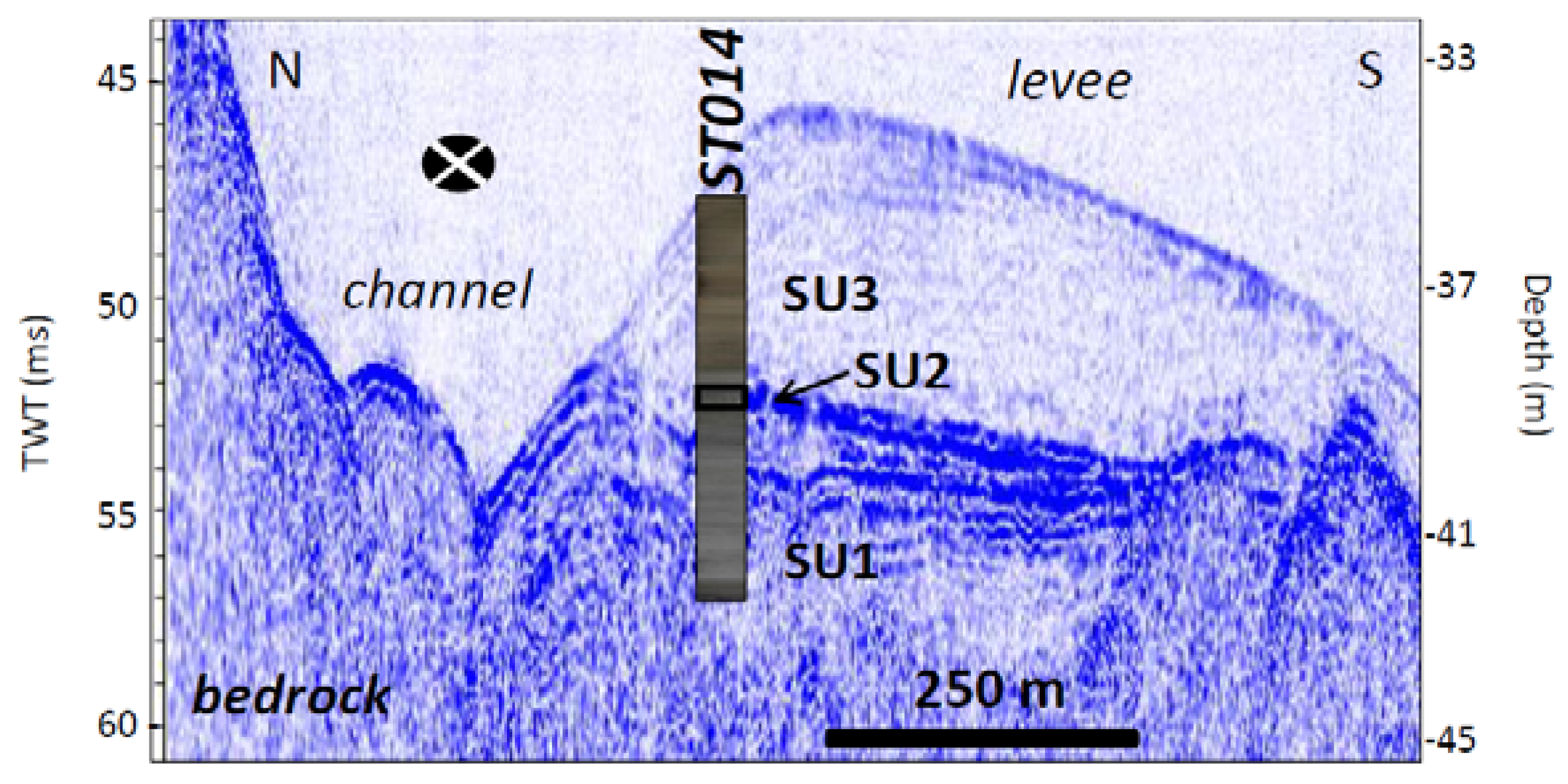
2.2. Seismic Survey
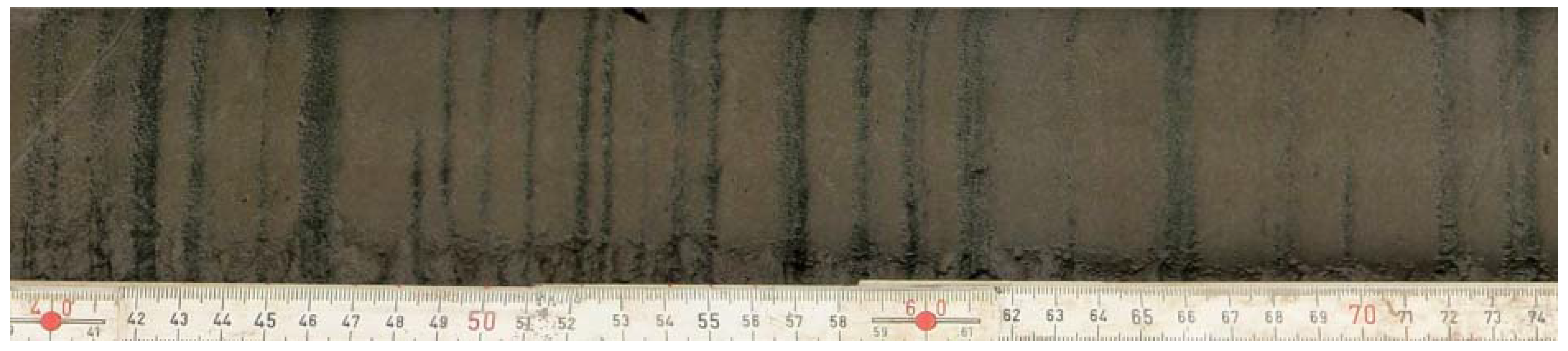
2.3. Sediment Coring
2.4. Core Correlation
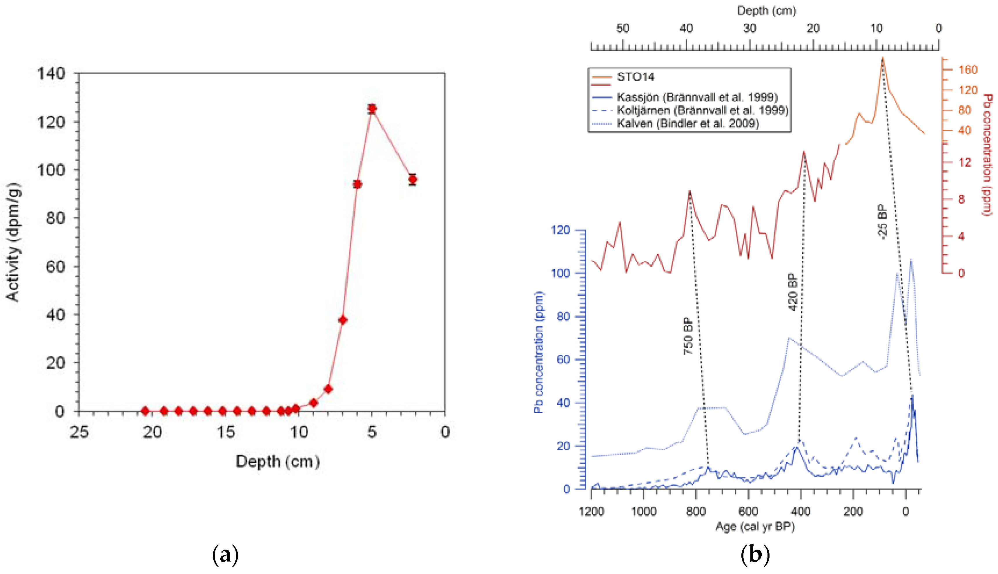
2.5. Dating and Age Modelling
2.6. Sediment Subsampling
2.7. Physical and Chemical Properties
2.8. Mineral Magnetic Properties
3. Results
3.1. Seismic Survey
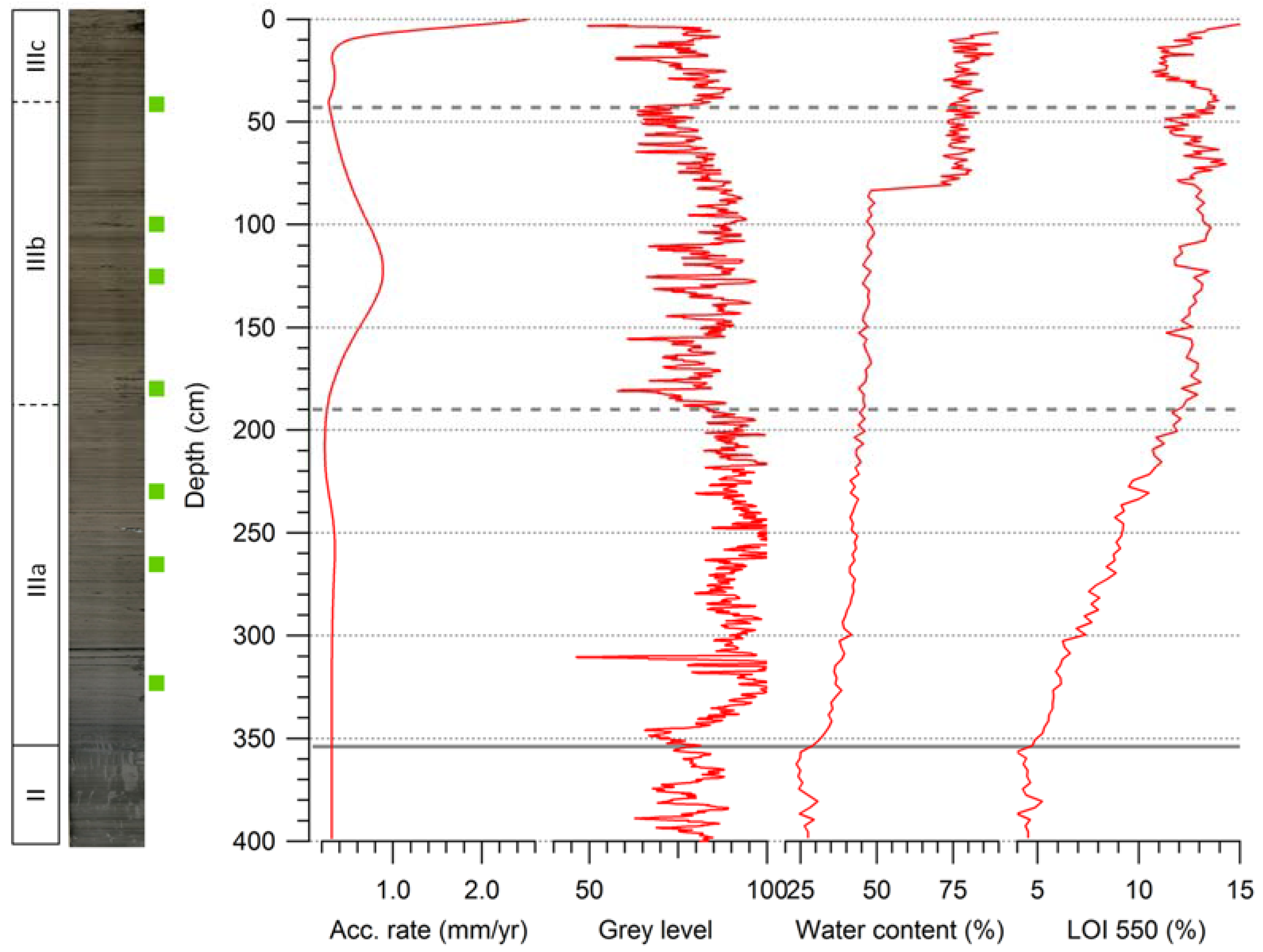
3.2. Lithological Description
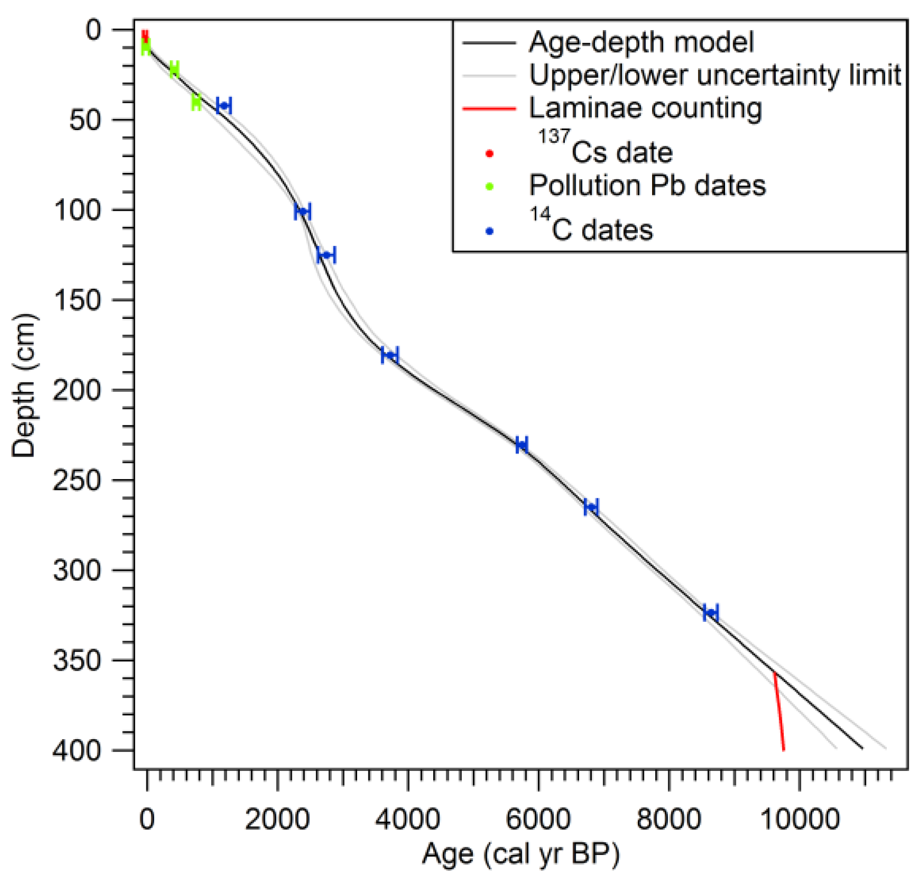
3.3. Age Model and Accumulation Rates
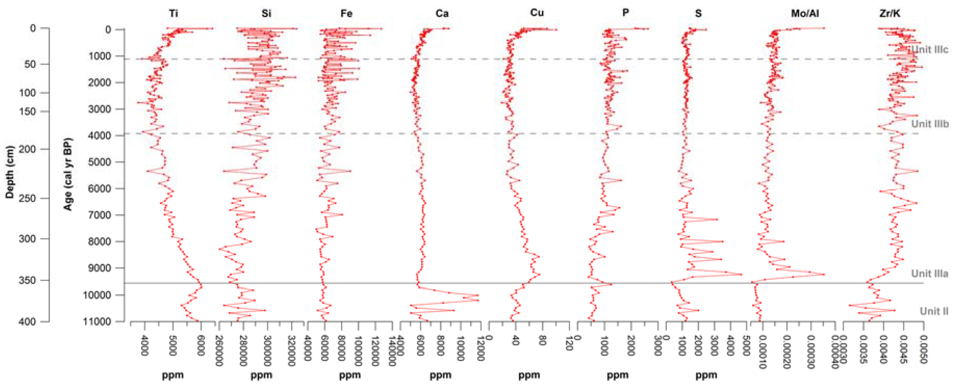
3.4. Chemical Sediment Properties
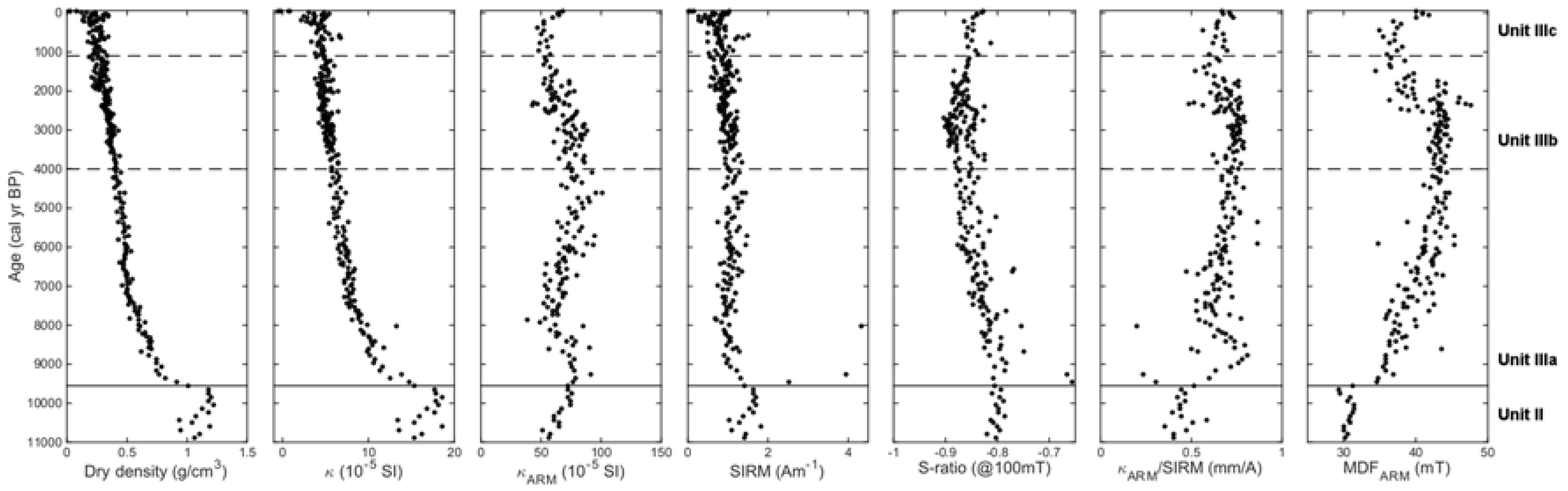
3.5. Mineral Magnetic Properties
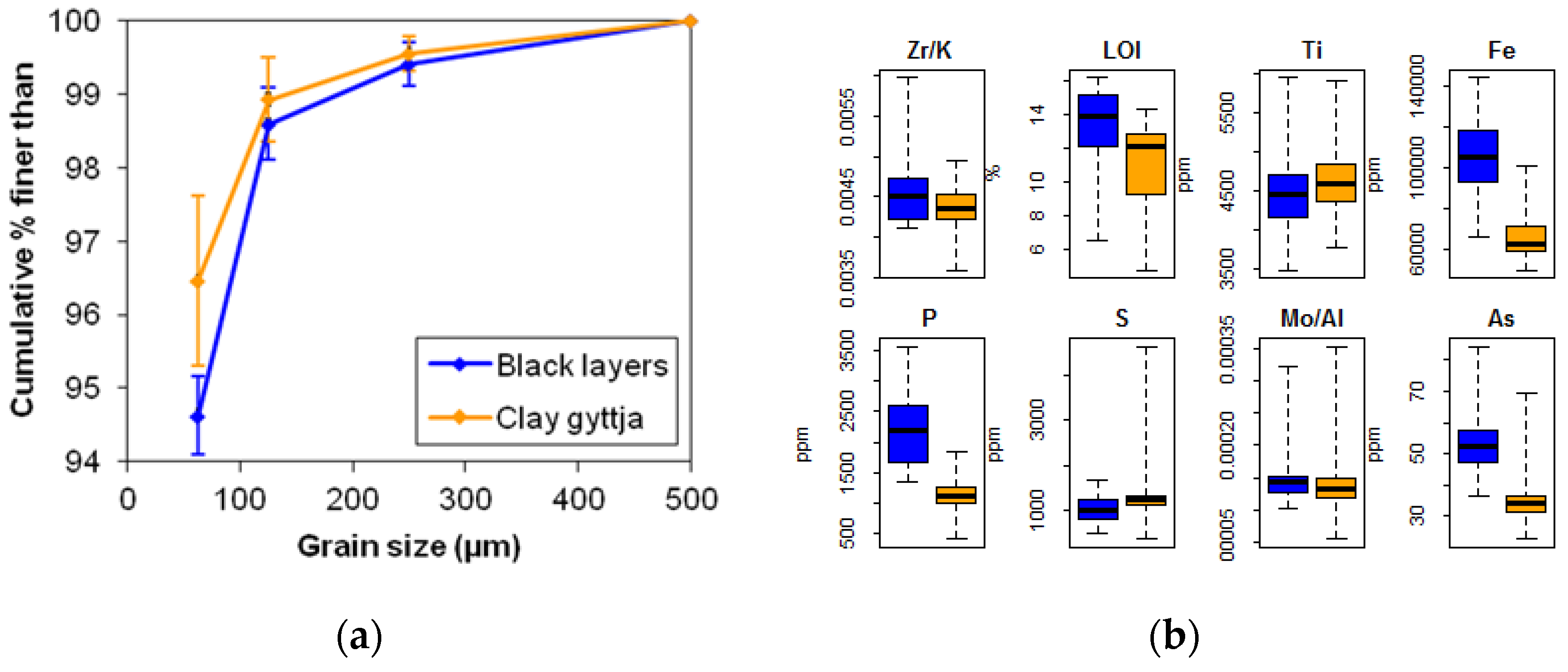
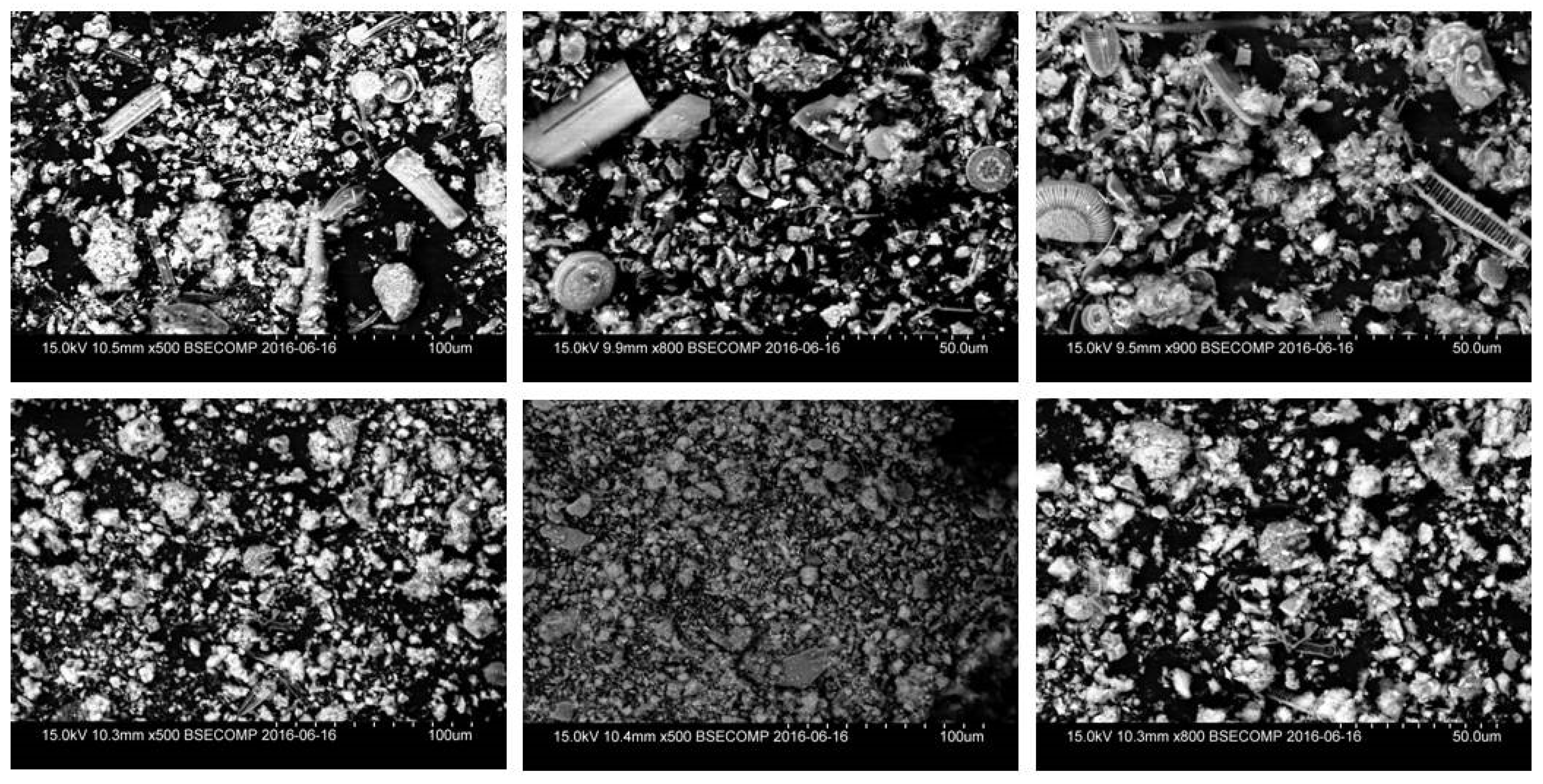
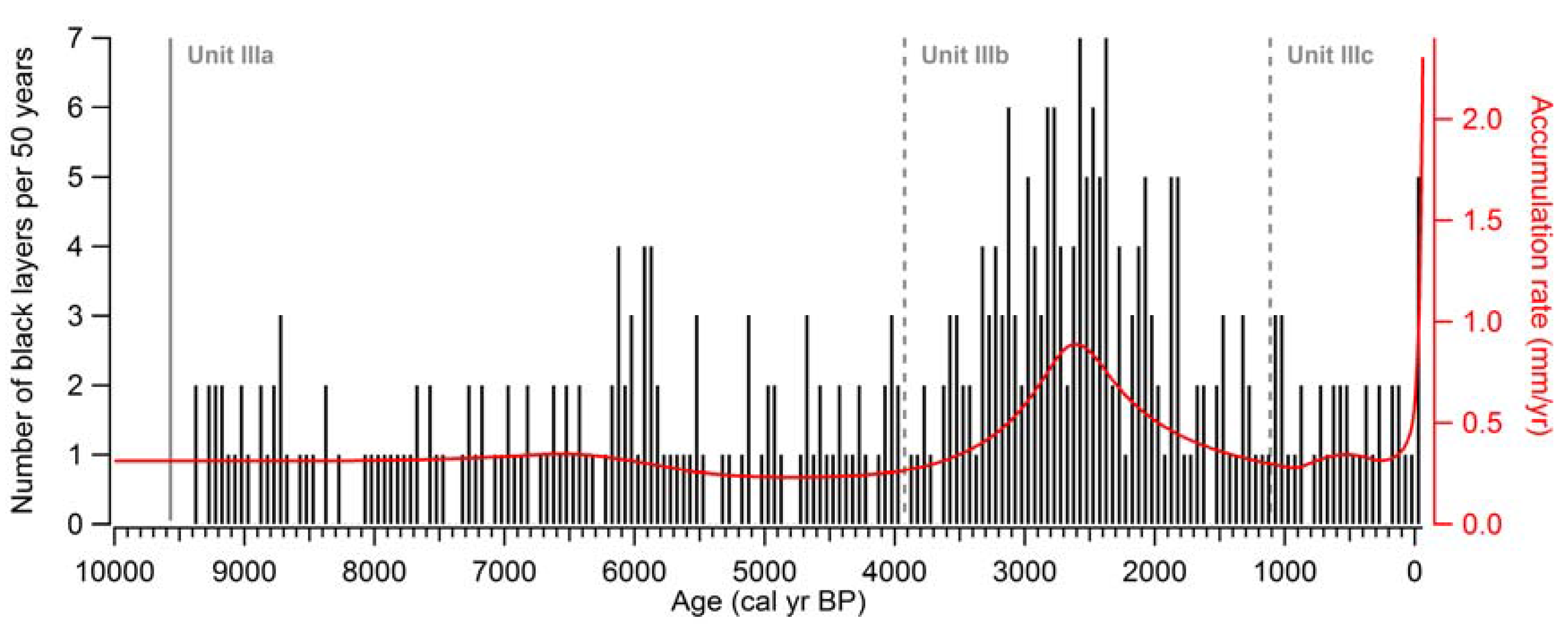
3.6. Characterization and Temporal Distribution of Black Layers
4. Discussion
4.1. Deglaciation and Early Postglacial Lake Development (Lithological Units I and II)
4.2. Lake and Catchment Processes During the Holocene (Lithological Unit III)
4.3. Palaeoenvironmental Significance of the Black Layers
4.3.1. Sediment Deposition at the Coring Site
4.3.2. Mechanisms of Black Layer Formation and Preservation
4.3.3. Relations to Climate and Vegetation Changes
5. Conclusions
Supplementary Materials
Acknowledgments
Author Contributions
Conflicts of Interest
References
- Nesje, A.; Matthews, J.A.; Dahl, S.O.; Berrisford, M.S.; Andersson, C. Holocene glacier fluctuations of Flatebreen and winter precipitation changes in the Jostedalsbreen region, western Norway, based on glaciolacustrine sediment records. Holocene 2001, 11, 267–280. [Google Scholar] [CrossRef]
- Hammarlund, D.; Björck, S.; Buchardt, B.; Israelson, C.; Thomsen, C.T. Rapid hydrological changes during the Holocene revealed by stable isotope records of lacustrine carbonates from Lake Igelsjön, southern Sweden. Quat. Sci. Rev. 2003, 22, 353–370. [Google Scholar] [CrossRef]
- Bjune, A.E.; Birks, H.J.B.; Seppä, H. Holocene vegetation and climate history on a continental-oceanic transect in northern Fennoscandia based on pollen and plant macrofossils. Boreas 2004, 33, 211–223. [Google Scholar] [CrossRef]
- Velle, G.; Brooks, S.J.; Birks, H.J.B.; Willassen, E. Chironomids as a tool for inferring Holocene climate: An assessment based on six sites in southern Scandinavia. Quat. Sci. Rev. 2005, 24, 1429–1462. [Google Scholar] [CrossRef]
- Andersson, S.; Rosqvist, G.; leng, M.J.; Wastegård, S.; Blaauw, M. Late Holocene climate change in central Sweden inferred from lacustrine stable isotope data. J. Quat. Sci. 2010, 25, 1305–1316. [Google Scholar] [CrossRef] [Green Version]
- Vasskog, K.; Nesje, A.; Støren, E.N.; Waldmann, N.; Chapron, E.; Ariztegui, D. A Holocene record of snow-avalanche and flood activity reconstructed from a lacustrine sedimentary sequence in Oldevatnet, western Norway. Holocene 2011, 21, 597–614. [Google Scholar] [CrossRef]
- Muschitiello, F.; Schwark, L.; Wohlfarth, B.; Sturm, C.; Hammarlund, D. New evidence of Holocene atmospheric circulation dynamics based on lake sediments from southern Sweden: A link to the Siberian High. Quat. Sci. Rev. 2013, 77, 113–124. [Google Scholar] [CrossRef]
- Rosén, P.; Segerström, U.; Eriksson, L.; Renberg, I.; Birks, H.J.B. Holocene climatic change reconstructed from diatoms, chironomids, pollen and near-infrared spectroscopy at an alpine lake (Sjuodjijaure) in northern Sweden. Holocene 2001, 11, 551–562. [Google Scholar] [CrossRef] [Green Version]
- Bigler, C.; Larocque, I.; Peglar, S.M.; Birks, H.J.B.; Hall, R.I. Quantitative multiproxy assessment of long-term patterns of Holocene environmental change from a small lake near Abisko, northern Sweden. Holocene 2002, 12, 481–496. [Google Scholar] [CrossRef] [Green Version]
- Hammarlund, D.; Barnekow, L.; Birks, H.J.B.; Buchardt, B.; Edwards, T.W.D. Holocene changes in atmospheric circulation recorded in the oxygen-isotope stratigraphy of lacustrine carbonates from northern Sweden. Holocene 2002, 12, 339–351. [Google Scholar] [CrossRef] [Green Version]
- Hammarlund, D.; Velle, G.; Wolfe, B.B.; Edwards, T.W.D.; Barnekow, L.; Bergman, J.; Holmgren, S.; Lamme, S.; Snowball, I.; Wohlfarth, B.; et al. Palaeolimnological and sedimentary responses to Holocene forest retreat in the Scandes Mountains, west-central Sweden. Holocene 2004, 14, 862–876. [Google Scholar] [CrossRef] [Green Version]
- Jonsson, C.E.; Andersson, S.; Rosqvist, G.C.; Leng, M.J. Reconstructing past atmospheric circulation changes using oxygen isotopes in lake sediments from Sweden. Clim. Past 2010, 6, 49–62. [Google Scholar] [CrossRef]
- Reuss, N.S.; Hammarlund, D.; Rundgren, M.; Segerström, U.; Eriksson, L.; Rosén, P. Lake Ecosystem Responses to Holocene Climate Change at the Subarctic Tree-Line in Northern Sweden. Ecosystems 2010, 13, 393–409. [Google Scholar] [CrossRef]
- St. Amour, N.A.; Hammarlund, D.; Edwards, T.W.D.; Wolfe, B.B. New insights into Holocene atmospheric circulation dynamics in central Scandinavia inferred from oxygen-isotope records of lake-sediment cellulose. Boreas 2010, 39, 770–782. [Google Scholar] [CrossRef]
- Meyer-Jacob, C.; Bindler, R.; Bigler, C.; Leng, M.J.; Lowick, S.E.; Vogel, H. Regional Holocene climate and landscape changes recorded in the large subarctic lake Torneträsk, N Fennoscandia. Palaeogeogr. Palaeoclimatol. Palaeoecol. 2017. [Google Scholar] [CrossRef]
- Von Grafenstein, U.; Erlenkeuser, H.; Brauer, A.; Jouzel, J.; Johnsen, S. A Mid-European Decadal Isotope-Climate Record from 15,500 to 5000 Years B.P. Science 1999, 284, 1654–1657. [Google Scholar] [CrossRef] [PubMed]
- Talbot, M.R.; Lærdal, T. The Late Pleistocene—Holocene palaeolimnology of Lake Victoria, East Africa, based upon elemental and isotopic analyses of sedimentary organic matter. J. Paleolimnol. 2000, 23, 141–164. [Google Scholar] [CrossRef]
- Arnaud, F.; Revel, M.; Chapron, E.; Desmet, M.; Tribovillard, N. 7200 years of Rhône River flooding activity in Lake Le Bourget, France: A high-resolution sediment record of NW Alps hydrology. Holocene 2005, 15, 420–428. [Google Scholar] [CrossRef] [Green Version]
- Chapron, E.; Arnaud, F.; Noël, H.; Revel, M.; Desmet, M.; Perdereau, L. Rhone River flood deposits in Lake Le Bourget: A proxy for Holocene environmental changes in the NW Alps, France. Boreas 2005, 34, 404–416. [Google Scholar] [CrossRef]
- Statens Offentliga Utredningar (SOU). Sweden Facing Climate Change—Threats and Opportunities; Swedish Government Official Reports; SOU: Stockholm, Sweden, 2007. [Google Scholar]
- Kochel, R.C.; Baker, V.R. Paleoflood Hydrology. Science 1982, 215, 353–361. [Google Scholar] [CrossRef] [PubMed]
- Mudelsee, M.; Börngen, M.; Tetzlaff, G.; Grünewald, U. No upward trends in the occurrence of extreme floods in central Europe. Nature 2003, 425, 166–169. [Google Scholar] [CrossRef] [PubMed]
- Debret, M.; Chapron, E.; Desmet, M.; Rolland-Revel, M.; Magand, O.; Trentesaux, A.; Bout-Roumazeille, V.; Nomade, J.; Arnaud, F. North western Alps Holocene paleohydrology recorded by flooding activity in Lake Le Bourget, France. Quat. Sci. Rev. 2010, 29, 2185–2200. [Google Scholar] [CrossRef] [Green Version]
- Støren, E.N.; Kolstad, E.W.; Paasche, Ø. Linking past flood frequencies in Norway to regional atmospheric circulation anomalies. J. Quat. Sci. 2012, 27, 71–80. [Google Scholar] [CrossRef]
- Czymzik, M.; Muscheler, R.; Brauer, A. Solar modulation of flood frequency in central Europe during spring and summer on interannual to multi-centennial timescales. Clim. Past 2016, 12, 799–805. [Google Scholar] [CrossRef]
- Simonneau, A.; Chapron, E.; Vannière, B.; Wirth, S.B.; Gilli, A.; Di Giovanni, C.; Anselmetti, F.S.; Desmet, M.; Magny, M. Mass-movement and flood-induced deposits in Lake Ledro, southern Alps, Italy: Implications for Holocene palaeohydrology and natural hazards. Clim. Past 2013, 9, 825–840. [Google Scholar] [CrossRef] [Green Version]
- Vannière, B.; Magny, M.; Joannin, S.; Simonneau, A.; Wirth, S.B.; Hamann, Y.; Chapron, E.; Gilli, A.; Desmet, M.; Anselmetti, F.S. Orbital changes, variation in solar activity and increased anthropogenic activities: Controls on the Holocene flood frequency in the Lake Ledro area, Northern Italy. Clim. Past 2013, 9, 1193–1209. [Google Scholar] [CrossRef] [Green Version]
- Wilhelm, B.; Arnaud, F.; Sabatier, P.; Magand, O.; Chapron, E.; Courp, T.; Tachikawa, K.; Fanget, B.; Malet, E.; Pignol, C.; et al. Palaeoflood activity and climate change over the last 1400 years recorded by lake sediments in the north-west European Alps. J. Quat. Sci. 2013, 28, 189–199. [Google Scholar] [CrossRef] [Green Version]
- Wirth, S.B.; Glur, L.; Gilli, A.; Anselmetti, F.S. Holocene flood frequency across the Central Alps—Solar forcing and evidence for variations in North Atlantic atmospheric circulation. Quat. Sci. Rev. 2013, 80, 112–128. [Google Scholar] [CrossRef]
- Sturm, M.; Matter, A. Turbidites and Varves in Lake Brienz (Switzerland): Deposition of Clastic Detritus by Density Currents. In Modern and Ancient Lake Sediments; Matter, A., Tucker, M.E., Eds.; Blackwell: Oxford, UK, 1978; pp. 147–168. ISBN 9781444303698. [Google Scholar]
- Mulder, T.; Chapron, E. Flood deposits in continental and marine environments: Character and significance. In Sediment Tranfer from Shelf to Deep Water-Revisiting the Delivery System; Slatt, R.M., Zavala, C., Eds.; American Association of Petroleum Geologists: Tulsa, OK, USA, 2011; pp. 1–30. [Google Scholar]
- Czymzik, M.; Dulski, P.; Plessen, B.; von Grafenstein, U.; Naumann, R.; Brauer, A. A 450 year record of spring-summer flood layers in annually laminated sediments from Lake Ammersee (southern Germany). Water Resour. Res. 2010, 46. [Google Scholar] [CrossRef]
- Schröder, H.G.; Wessels, M.; Niessen, F. Acoustic facies and depositional structures of Lake Constance. Ergebnisse der Limnolog. 1999, 53, 351–368. [Google Scholar]
- Schneider, J.L.; Pollet, N.; Chapron, E.; Wessels, M.; Wassmer, P. Signature of Rhine Valley sturzstrom dam failures in Holocene sediments of Lake Constance, Germany. Sediment. Geol. 2004, 169, 75–91. [Google Scholar] [CrossRef]
- Girardclos, S.; Baster, I.; Wildi, W.; Pugin, A.; Rachoud-Schneider, A.-M. Bottom-current and wind-pattern changes as indicated by Late Glacial and Holocene sediments from western Lake Geneva (Switzerland). In Lake Systems from the Ice Age to Industrial Time; Birkhäuser Basel: Basel, Switzerland, 2003; pp. 39–48. [Google Scholar]
- Girardclos, S.; Fiore, J.; Rachoud-Schneider, A.-M.; Baster, I.; Wildo, W. Petit-Lac (western Lake Geneva) environment and climate history from deglaciation to the present: A synthesis. Boreas 2005, 34, 417–433. [Google Scholar] [CrossRef]
- Chapron, E.; Van Rensbergen, P.; De Batist, M.; Beck, C.; Henriet, J.P. Fluid-escape features as a precursor of a large sublacustrine sediment slide in Lake Le Bourget, NW Alps, France. Terra Nova 2004, 16, 305–311. [Google Scholar] [CrossRef]
- Gilli, A.; Anselmetti, F.S.; Ariztegui, D.; Beres, M.; McKenzie, J.A.; Markgraf, V. Seismic stratigraphy, buried beach ridges and contourite drifts: The Late Quaternary history of the closed Lago Cardiel basin, Argentina (49° S). Sedimentology 2005, 52, 1–23. [Google Scholar] [CrossRef]
- Gilli, A.; Ariztegui, D.; Anselmetti, F.S.; McKenzie, J.A.; Markgraf, V.; Hajdas, I.; McCulloch, R.D. Mid-Holocene strengthening of the Southern Westerlies in South America—Sedimentological evidences from Lago Cardiel, Argentina (49° S). Glob. Planet. Chang. 2005, 49, 75–93. [Google Scholar] [CrossRef]
- Kremer, K.; Corella, J.P.; Hilbe, M.; Marillier, F.; Dupuy, D.; Zenhäusern, G.; Girardclos, S. Changes in distal sedimentation regime of the Rhone delta system controlled by subaquatic channels (Lake Geneva, Switzerland/France). Mar. Geol. 2015, 370, 125–135. [Google Scholar] [CrossRef]
- Johnson, T.C. Late-glacial and postglacial sedimentation in Lake Superior based on seismic-reflection profiles. Quat. Res. 1980, 13, 380–391. [Google Scholar] [CrossRef]
- Johnson, T.C. Sedimentary processes and signals of past climate change in the large lakes of the East African Rift Valley. In The Limnology, Climatology and Paleoclimatology of the East African Lakes; Johnson, T.C., Odada, E.O., Eds.; Gordon & Breach: Amsterdam, The Netherlands, 1996; p. 664. [Google Scholar]
- Ceramicola, S.; Rebesco, M.; De Batist, M.; Khlystov, O. Seismic evidence of small-scale lacustrine drifts in Lake Baikal (Russia). Mar. Geophys. Res. 2001, 22, 445–464. [Google Scholar] [CrossRef]
- Lundqvist, J. Weichsel-istidens huvudfas. In Berg och jord; Fredén, C., Ed.; Sveriges Nationalatlas: Stockholm, Sweden, 2009; p. 208. [Google Scholar]
- Hallberg, K.; Wänström, M.; Edman, A. Circulationsmodell Storsjön (Circulation Model Storsjön); SMHI Report No. 2015-17; Swedish Meteorological and Hydrological Institute: Stockholm, Sweden, 2015. [Google Scholar]
- SMHI (Swedish Meteorological and Hydrological Institute). Vattenwebb. Available online: vattenwebb.smhi.se (accessed on 15 May 2017).
- Renberg, I.; Hansson, H. Freeze corer No. 3 for lake sediments. J. Paleolimnol. 2010, 44, 731–736. [Google Scholar] [CrossRef]
- Cottereau, E.; Arnold, M.; Moreau, C.; Baqué, D.; Bavay, D.; Caffy, I.; Comby, C.; Dumoulin, J.-P.; Hain, S.; Perron, M.; et al. Artemis, the New 14C AMS at LMC14 in Saclay, France. Radiocarbon 2007, 49, 291–299. [Google Scholar] [CrossRef]
- Moreau, C.; Caffy, I.; Comby, C.; Delqué-Količ, E.; Dumoulin, J.-P.; Hain, S.; Quiles, A.; Setti, V.; Souprayen, C.; Thellier, B.; et al. Research and Development of the Artemis 14C AMS Facility: Status Report. Radiocarbon 2013, 55, 331–337. [Google Scholar] [CrossRef]
- Dumoulin, J.-P.; Comby-Zerbino, C.; Delqué-Količ, E.; Moreau, C.; Caffy, I.; Hain, S.; Perron, M.; Thellier, B.; Setti, V.; Berthier, B.; et al. Status Report on Sample Preparation Protocols Developed at the LMC14 Laboratory, Saclay, France: From Sample Collection to 14C AMS Measurement. Radiocarbon 2017, 59, 713–726. [Google Scholar] [CrossRef]
- Reimer, P.; Bard, E.; Bayliss, A. IntCal13 and Marine13 radiocarbon age calibration curves 0--50,000 years cal BP. Radiocarbon 2013, 55, 1869–1887. [Google Scholar] [CrossRef] [Green Version]
- Weiss, D.; Shotyk, W.; Appleby, P.G.; Kramers, J.D.; Cheburkin, A.K. Atmospheric Pb Deposition since the Industrial Revolution Recorded by Five Swiss Peat Profiles: Enrichment Factors, Fluxes, Isotopic Composition and Sources. Environ. Sci. Technol. 1999, 33, 1340–1352. [Google Scholar] [CrossRef]
- Brännvall, M.-L.; Bindler, R.; Renberg, I.; Emteryd, O.; Bartnicki, J.; Billström, K. The Medieval metal industry was the cradle of modern large-scale atmospheric lead pollution in Northern Europe. Environ. Sci. Technol. 1999, 33, 4391–4395. [Google Scholar] [CrossRef]
- Boës, X.; Rydberg, J.; Martinez-Cortizas, A.; Bindler, R.; Renberg, I. Evaluation of conservative lithogenic elements (Ti, Zr, Al, and Rb) to study anthropogenic element enrichments in lake sediments. Journal of Paleolimnology 2011, 46, 75–87. [Google Scholar] [CrossRef]
- Cutshall, N.H.; Larsen, I.L.; Olsen, C.R. Direct analysis of 210Pb in sediment samples: Self-absorption corrections. Nucl. Instrum. Methods 1983, 306, 309–312. [Google Scholar] [CrossRef]
- Blaauw, M. Methods and code for “classical” age-modelling of radiocarbon sequences. Quaternary Geochronology 2010, 5, 512–518. [Google Scholar] [CrossRef]
- Heiri, O.; Lotter, A.; Lemcke, G. Loss on ignition as a method for estimating organic and carbonate content in sediments: Reproducibility and comparability of results. J. Paleolimnol. 2001, 25, 101–110. [Google Scholar] [CrossRef]
- Vogel, H.; Wagner, B.; Rosén, P. Lake floor morphology and sediment architecture of lake Torneträsk, northern Sweden. Geogr. Ann. Ser. A Phys. Geogr. 2013, 95, 159–170. [Google Scholar] [CrossRef]
- Ritchie, J.C.; McHenry, J.R. Application of Radioactive Fallout Cesium-137 for Measuring Soil Erosion and Sediment Accumulation Rates and Patterns: A Review. J. Environ. Qual. 1990, 19, 215–233. [Google Scholar] [CrossRef]
- Jarvis, N.J.; Taylor, A.; Larsbo, M.; Etana, A.; Rosén, K. Modelling the effects of bioturbation on the re-distribution of 137Cs in an undisturbed grassland soil. Eur. J. Soil Sci. 2010, 61, 24–34. [Google Scholar] [CrossRef]
- Klaminder, J.; Appleby, P.; Crook, P.; Renberg, I. Post-deposition diffusion of 137Cs in lake sediment: Implications for radiocaesium dating. Sedimentology 2012, 59, 2259–2267. [Google Scholar] [CrossRef]
- Renberg, I.; Persson, M.W.; Emteryd, O. Pre-industrial atmospheric lead contamination detected in Swedish lake sediments. Nature 1994, 368, 323–326. [Google Scholar] [CrossRef]
- Renberg, I.; Bindler, R.; Brannvall, M.L. Using the historical atmospheric lead-deposition record as a chronological marker in sediment deposits in Europe. Holocene 2001, 11, 511–516. [Google Scholar] [CrossRef]
- Bindler, R.; Renberg, I.; Rydberg, J.; Andrén, T. Widespread waterborne pollution in central Swedish lakes and the Baltic Sea from pre-industrial mining and metallurgy. Environ. Pollut. 2009, 157, 2132–2141. [Google Scholar] [CrossRef] [PubMed]
- Andrén, T.; Björck, J.; Johnsen, S. Correlation of Swedish glacial varves with the Greenland (GRIP) oxygen isotope record. J. Quat. Sci. 1999, 14, 361–371. [Google Scholar] [CrossRef]
- Petterson, G. Varved sediments in Sweden: A brief review. Geol. Soc. Lond. Spec. Publ. 1996, 116, 73–77. [Google Scholar] [CrossRef]
- Cunningham, L.; Vogel, H.; Wennrich, V.; Juschus, O.; Nowaczyk, N.; Rosén, P. Amplified bioproductivity during Transition IV (332,000–342,000 years ago): Evidence from the geochemical record of Lake El’gygytgyn. Clim. Past 2013, 9, 679–686. [Google Scholar] [CrossRef] [Green Version]
- Cuven, S.; Francus, P.; Lamoureux, S.F. Estimation of grain size variability with micro X-ray fluorescence in laminated lacustrine sediments, Cape Bounty, Canadian high arctic. J. Paleolimnol. 2010, 44, 803–817. [Google Scholar] [CrossRef]
- Dean, W.E.; Piper, D.Z.; Peterson, L.C. Molybdenum accumulation in Cariaco basin sediment over the past 24 k.y.: A record of water-column anoxia and climate. Geology 1999, 27, 507–510. [Google Scholar] [CrossRef]
- Chappaz, A.; Gobeil, C.; Tessier, A. Geochemical and anthropogenic enrichments of Mo in sediments from perennially oxic and seasonally anoxic lakes in Eastern Canada. Geochim. Cosmochim. Acta 2008, 72, 170–184. [Google Scholar] [CrossRef]
- Snowball, I.; Thompson, R. A stable chemical remanence in Holocene sediments. J. Geophys. Res. 1990, 95, 4471. [Google Scholar] [CrossRef]
- Maher, B.A. Magnetic properties of some synthetic sub-micron magnetites. Geophys. J. Int. 1988, 94, 83–96. [Google Scholar] [CrossRef]
- Oldfield, F. Toward the discrimination of fine-grained ferrimagnets by magnetic measurements in lake and near-shore marine sediments. J. Geophys. Res. Solid Earth 1994, 99, 9045–9050. [Google Scholar] [CrossRef]
- Egli, R. Characterization of Individual Rock Magnetic Components by Analysis of Remanence Curves, 1. Unmixing Natural Sediments. Stud. Geophys. Geod. 2004, 48, 391–446. [Google Scholar] [CrossRef]
- Moskowitz, B.M.; Frankel, R.B.; Bazylinski, D.A. Rock magnetic criteria for the detection of biogenic magnetite. Earth Planet. Sci. Lett. 1993, 120, 283–300. [Google Scholar] [CrossRef]
- Snowball, I.; Zillén, L.; Sandgren, P. Bacterial magnetite in Swedish varved lake-sediments: A potential bio-marker of environmental change. Quat. Int. 2002, 88, 13–19. [Google Scholar] [CrossRef]
- Stroeven, A.P.; Hättestrand, C.; Kleman, J.; Heyman, J.; Fabel, D.; Fredin, O.; Goodfellow, B.W.; Harbor, J.M.; Jansen, J.D.; Olsen, L.; et al. Deglaciation of Fennoscandia. Quat. Sci. Rev. 2016, 147, 91–121. [Google Scholar] [CrossRef] [Green Version]
- Lundqvist, J. Isavsmältningens Förlopp i Jämtlands län; Sveriges Geologiska Undersökning: Uppsala, Sweden, 1973; Volume 66, p. 187. [Google Scholar]
- Johnsen, T.F. Late Quaternary Ice Sheet History and Dynamics in Central and Southern Scandinavia. Ph.D. Thesis, Stockholm University, Stockholm, Sweden, 2010. [Google Scholar]
- Lundqvist, J. Ice-lake types and deglaciation pattern along the Scandinavian mountain range. Boreas 1972, 1, 27–54. [Google Scholar] [CrossRef]
- Borgström, I. Terrängformerna och den Glaciala Utvecklingen i Södra Fjällen; Stockholm University: Stockholm, Sweden, 1989. [Google Scholar]
- Moscariello, A.; Pugin, A.; Wildi, W.; Beck, C.; Chapron, E.; De Batist, M.; Girardclos, S.; Ivy Ochs, S.; Rachoud-Schneider, A.M.; Signer, C.; et al. Déglaciation würmienne dans des conditions lacustres à la terminaison occidentale du bassin lémanique (Suisse occidentale et France). Eclogae Geol. Helv. 1998, 91, 185–201. [Google Scholar] [CrossRef]
- Van Rensbergen, P.; De Batist, M.; Beck, C.; Manalt, F. High-resolution seismic stratigraphy of late quaternary fill of Lake Annecy (northwestern Alps): Evolution from glacial to interglacial sedimentary processes. Sediment. Geol. 1998, 117, 71–96. [Google Scholar] [CrossRef]
- Van Rensbergen, P.; de Batist, M.; Beck, C.; Chapron, E. High-resolution seismic stratigraphy of glacial to interglacial fill of a deep glacigenic lake: Lake Le Bourget, Northwestern Alps, France. Sediment. Geol. 1999, 128, 99–129. [Google Scholar] [CrossRef]
- Peach, P.A.; Perrie, L.A. Grain-Size Distribution within Glacial Varves. Geology 1975, 3, 43. [Google Scholar] [CrossRef]
- Ridge, J.C.; Balco, G.; Bayless, R.L.; Beck, C.C.; Carter, L.B.; Dean, J.L.; Voytek, E.B.; Wei, J.H. The new North American Varve Chronology: A precise record of southeastern Laurentide Ice Sheet deglaciation and climate, 18.2-12.5 kyr BP and correlations with Greenland ice core records. Am. J. Sci. 2012, 312, 685–722. [Google Scholar] [CrossRef]
- Piper, D.Z.; Isaacs, C.M. Geochemistry of Mi-Nor Elements in the Monterey Formation, California: Seawater Chemistry of Deposition; US Geological Survey Professional Paper 1556; USGS: Reston, VA, USA, 1995; Volume 1566, pp. 1–41.
- Bergman, J.; Hammarlund, D.; Hannon, G.; Barnekow, L.; Wohlfarth, B. Deglacial vegetation succession and Holocene tree-limit dynamics in the Scandes Mountains, west-central Sweden: Stratigraphic data compared to megafossil evidence. Rev. Palaeobot. Palynol. 2005, 134, 129–151. [Google Scholar] [CrossRef]
- Antonsson, H. The extent of farm desertion in central Sweden during the late medieval agrarian crisis: Landscape as a source. J. Hist. Geogr. 2009, 35, 619–641. [Google Scholar] [CrossRef]
- Karlsson, J.; Rydberg, J.; Segerström, U.; Nordström, E.-M.; Thöle, P.; Biester, H.; Bindler, R. Tracing a bog-iron bloomery furnace in an adjacent lake-sediment record in Ängersjö, central Sweden, using pollen and geochemical signals. Veg. Hist. Archaeobot. 2016, 25, 569–581. [Google Scholar] [CrossRef]
- Smol, J.P.; Wolfe, A.P.; Birks, H.J.B.; Douglas, M.S.V.; Jones, V.J.; Korhola, A.; Pienitz, R.; Ruhland, K.; Sorvari, S.; Antoniades, D.; et al. Climate-driven regime shifts in the biological communities of arctic lakes. Proc. Natl. Acad. Sci. USA 2005, 102, 4397–4402. [Google Scholar] [CrossRef] [PubMed]
- Waters, C.N.; Zalasiewicz, J.; Summerhayes, C.; Barnosky, A.D.; Poirier, C.; Galuszka, A.; Cearreta, A.; Edgeworth, M.; Ellis, E.C.; Ellis, M.; et al. The Anthropocene is functionally and stratigraphically distinct from the Holocene. Science 2016, 351. [Google Scholar] [CrossRef] [PubMed]
- Ek, A.S.; Renberg, I. Heavy metal pollution and lake acidity changes caused by one thousand years of copper mining at Falun, central Sweden. J. Paleolimnol. 2001, 26, 89–107. [Google Scholar] [CrossRef]
- Rebesco, M.; Hernández-Molina, F.J.; Van Rooij, D.; Wåhlin, A. Contourites and associated sediments controlled by deep-water circulation processes: State-of-the-art and future considerations. Mar. Geol. 2014, 352, 111–154. [Google Scholar] [CrossRef] [Green Version]
- Mulder, T.; Syvitski, J.P.M.; Migeon, S.; Faugères, J.-C.; Savoye, B. Marine hyperpycnal flows: Initiation, behavior and related deposits. A review. Mar. Pet. Geol. 2003, 20, 861–882. [Google Scholar] [CrossRef]
- Chapron, E.; Desmet, M.; De Putter, T.; Loutre, M.F.; Beck, C.; Deconinck, J.F. Climatic variability in the northwestern Alps, France, as evidenced by 600 years of terrigenous sedimentation in Lake Le Bourget. Holocene 2002, 12, 177–185. [Google Scholar] [CrossRef]
- Odegaard, C.; Rea, D.K.; Moore, T.C. Stratigraphy of the mid-Holocene black bands in Lakes Michigan and Huron: Evidence for possible basin-wide anoxia. J. Paleolimnol. 2003, 29, 221–234. [Google Scholar] [CrossRef]
- Pitkänen, H.; Lehtoranta, J.; Räike, A. Internal Nutrient in External Load: Of Eastern Gulf Fluxes Counteract Decreases The Case of the Estuarial Eastern Gulf of Finland, Baltic Sea. Ambio 2001, 30, 195–201. [Google Scholar] [CrossRef] [PubMed]
- Granina, L.; Müller, B.; Wehrli, B. Origin and dynamics of Fe and Mn sedimentary layers in Lake Baikal. Chem. Geol. 2004, 205, 55–72. [Google Scholar] [CrossRef]
- Sander, M.; Bengtsson, L.; Holmquist, B.; Wohlfarth, B.; Cato, I. The relationship between annual varve thickness and maximum annual discharge (1909–1971). J. Hydrol. 2002, 263, 23–35. [Google Scholar] [CrossRef]
- Haltia-Hovi, E.; Saarinen, T.; Kukkonen, M. A 2000-year record of solar forcing on varved lake sediment in eastern Finland. Quat. Sci. Rev. 2007, 26, 678–689. [Google Scholar] [CrossRef]
- Ojala, A.E.K.; Alenius, T. 10,000 Years of interannual sedimentation recorded in the Lake Nautajärvi (Finland) clastic-organic varves. Palaeogeogr. Palaeoclimatol. Palaeoecol. 2005, 219, 285–302. [Google Scholar] [CrossRef]
- Rothwell, R.G.; Hoogakker, B.; Thomson, J.; Croudace, I.W.; Frenz, M. Turbidite emplacement on the southern Balearic Abyssal Plain (western Mediterranean Sea) during Marine Isotope Stages 1–3: An application of ITRAX XRF scanning of sediment cores to lithostratigraphic analysis. In New Techniques in Sediment Core Analysis; Rothwell, R.G., Ed.; Geological Society: London, UK, 2006; Volume 267, pp. 79–98. [Google Scholar]
- Huerta-Diaz, M.A.; Morse, J.W. Pyritization of trace metals in anoxic sediments. Geochim. Cosmochim. Acta 1992, 56, 2681–2702. [Google Scholar] [CrossRef]
- Rothe, M.; Frederichs, T.; Eder, M.; Kleeberg, A.; Hupfer, M. Evidence for vivianite formation and its contribution to long-term phosphorus retention in a recent lake sediment: A novel analytical approach. Biogeosciences 2014, 11, 5169–5180. [Google Scholar] [CrossRef] [Green Version]
- Manning, P.G.; Murphy, T.P.; Prepas, E.E. Intensive formation of vivianite in the bottom sediments of mesotrophic Narrow Lake, Alberta. Can. Mineral. 1991, 29, 77–85. [Google Scholar]
- O’Connell, D.W.; Mark Jensen, M.; Jakobsen, R.; Thamdrup, B.; Joest Andersen, T.; Kovacs, A.; Bruun Hansen, H.C. Vivianite formation and its role in phosphorus retention in Lake Ørn, Denmark. Chem. Geol. 2015, 409, 42–53. [Google Scholar] [CrossRef]
- Kullman, L.; Kjällgren, L. Holocene pine tree-line evolution in the Swedish Scandes: Recent tree-line rise and climate change in a long-term perspective. Boreas 2006, 35, 159–168. [Google Scholar] [CrossRef]
- Kullman, L. Ecological tree line history and palaeoclimate—Review of megafossil evidence from the Swedish Scandes. Boreas 2013, 42, 555–567. [Google Scholar] [CrossRef]
- Barnekow, L.; Bragée, P.; Hammarlund, D.; St. Amour, N. Boreal forest dynamics in north-eastern Sweden during the last 10,000 years based on pollen analysis. Veg. Hist. Archaeobot. 2008, 17, 687–700. [Google Scholar] [CrossRef]
- SMHI (Swedish Meteorological and Hydrological Institute). Översvämningar i Sverige (Floods in Sweden); SMHI: Stockholm, Sweden, 2004. [Google Scholar]
- Sander, M. Climatic Signals and Frequencies in the Swedish Time Scale, River Ångermanälven, Central Sweden; Lund University: Lund, Sweden, 2003. [Google Scholar]
- Støren, E.N.; Paasche, Ø. Scandinavian floods: From past observations to future trends. Glob. Planet. Chang. 2014, 113, 34–43. [Google Scholar] [CrossRef]
- Martin-Puertas, C.; Matthes, K.; Brauer, A.; Muscheler, R.; Hansen, F.; Petrick, C.; Aldahan, A.; Possnert, G.; van Geel, B. Regional atmospheric circulation shifts induced by a grand solar minimum. Nat. Geosci. 2012, 5, 397–401. [Google Scholar] [CrossRef]
- Holzhauser, H.; Magny, M.; Zumbühl, H.J. Glacier and lake-level variations in west-central Europe over the last 3500 years. Holocene 2005, 15, 789–801. [Google Scholar] [CrossRef]
- Kroonenberg, S.B.; Abdurakhmanov, G.M.; Badyukova, E.N.; van der Borg, K.; Kalashnikov, A.; Kasimov, N.S.; Rychagov, G.I.; Svitoch, A.A.; Vonhof, H.B.; Wesselingh, F.P. Solar-forced 2600 BP and Little Ice Age highstands of the Caspian Sea. Quat. Int. 2007, 173–174, 137–143. [Google Scholar] [CrossRef]
- Mauquoy, D.; Yeloff, D.; Van Geel, B.; Charman, D.J.; Blundell, A. Two decadally resolved records from north-west European peat bogs show rapid climate changes associated with solar variability during the mid-late Holocene. J. Quat. Sci. 2008, 23, 745–763. [Google Scholar] [CrossRef]
- Czymzik, M.; Brauer, A.; Dulski, P.; Plessen, B.; Naumann, R.; von Grafenstein, U.; Scheffler, R. Orbital and solar forcing of shifts in Mid- to Late Holocene flood intensity from varved sediments of pre-alpine Lake Ammersee (southern Germany). Quat. Sci. Rev. 2013, 61, 96–110. [Google Scholar] [CrossRef]
- Van Geel, B.; Heijnis, H.; Charman, D.J.; Thompson, G.; Engels, S. Bog burst in the eastern Netherlands triggered by the 2.8 kyr BP climate event. Holocene 2014, 24, 1465–1477. [Google Scholar] [CrossRef]
- Mellström, A.; Van Der Putten, N.; Muscheler, R.; De Jong, R.; Björck, S. A shift towards wetter and windier conditions in southern Sweden around the prominent solar minimum 2750 cal a BP. J. Quat. Sci. 2015, 30, 235–244. [Google Scholar] [CrossRef]
- De Jong, R.; Hammarlund, D.; Nesje, A. Late Holocene effective precipitation variations in the maritime regions of south-west Scandinavia. Quat. Sci. Rev. 2009, 28, 54–64. [Google Scholar] [CrossRef]
- Faust, J.C.; Knies, J.; Milzer, G.; Giraudeau, J. Terrigenous input to a fjord in central Norway records the environmental response to the North Atlantic Oscillation over the past 50 years. Holocene 2014, 24, 1411–1418. [Google Scholar] [CrossRef]
- Cherry, J.; Cullen, H.; Visbeck, M.; Small, A.; Uvo, C. Impacts of the North Atlantic oscillation on Scandinavian hydropower production and energy markets. Water Resour. Manag. 2005, 19, 673–691. [Google Scholar] [CrossRef]
- Ineson, S.; Scaife, A.A.; Knight, J.R.; Manners, J.C.; Dunstone, N.J.; Gray, L.J.; Haigh, J.D. Solar forcing of winter climate variability in the Northern Hemisphere. Nat. Geosci. 2011, 4, 753–757. [Google Scholar] [CrossRef]
- Olsen, J.; Anderson, N.J.; Knudsen, M.F. Variability of the North Atlantic Oscillation over the past 5200 years. Nat. Geosci. 2012, 5, 808–812. [Google Scholar] [CrossRef]
- Bjune, A.E.; Bakke, J.; Nesje, A.; Birks, H.J.B. Holocene mean July temperature and winter precipitation in western Norway inferred from palynological and glaciological lake-sediment proxies. Holocene 2005, 15, 177–189. [Google Scholar] [CrossRef]


| Depth (cm) | Material | 14C Age BP ± Error | Cal. Age BP (2σ Range) | Lab. ID |
|---|---|---|---|---|
| 41.6 | Wood fragment | 1165 ± 30 | 985–1177 | SacA39831 |
| 100.4 | Twig | 2330 ± 30 | 2213–2431 | SacA39833 |
| 124.5 | Wood fragment | 2540 ± 30 | 2497–2747 | SacA39832 |
| 180.2 | Twig | 3410 ± 30 | 3577–3811 | SacA39834 |
| 229.8 | Wood fragments | 4950 ± 35 | 5603–5740 | SacA39836 |
| 264.4 | Twig | 5915 ± 40 | 6657–6847 | SacA39835 |
| 322.9 | Wood fragment | 7785 ± 45 | 8447–8639 | LuS11056 |
© 2018 by the authors. Licensee MDPI, Basel, Switzerland. This article is an open access article distributed under the terms and conditions of the Creative Commons Attribution (CC BY) license (http://creativecommons.org/licenses/by/4.0/).
Share and Cite
Labuhn, I.; Hammarlund, D.; Chapron, E.; Czymzik, M.; Dumoulin, J.-P.; Nilsson, A.; Régnier, E.; Robygd, J.; Von Grafenstein, U. Holocene Hydroclimate Variability in Central Scandinavia Inferred from Flood Layers in Contourite Drift Deposits in Lake Storsjön. Quaternary 2018, 1, 2. https://0-doi-org.brum.beds.ac.uk/10.3390/quat1010002
Labuhn I, Hammarlund D, Chapron E, Czymzik M, Dumoulin J-P, Nilsson A, Régnier E, Robygd J, Von Grafenstein U. Holocene Hydroclimate Variability in Central Scandinavia Inferred from Flood Layers in Contourite Drift Deposits in Lake Storsjön. Quaternary. 2018; 1(1):2. https://0-doi-org.brum.beds.ac.uk/10.3390/quat1010002
Chicago/Turabian StyleLabuhn, Inga, Dan Hammarlund, Emmanuel Chapron, Markus Czymzik, Jean-Pascal Dumoulin, Andreas Nilsson, Edouard Régnier, Joakim Robygd, and Ulrich Von Grafenstein. 2018. "Holocene Hydroclimate Variability in Central Scandinavia Inferred from Flood Layers in Contourite Drift Deposits in Lake Storsjön" Quaternary 1, no. 1: 2. https://0-doi-org.brum.beds.ac.uk/10.3390/quat1010002