Approach for Analysis of Land-Cover Changes and Their Impact on Flooding Regime


Department of Civil Engineering, The University of Tokyo, Tokyo 113-8654, Japan
Quaternary 2019, 2(3), 27; https://0-doi-org.brum.beds.ac.uk/10.3390/quat2030027
Submission received: 6 June 2019
/
Revised: 22 July 2019
/
Accepted: 26 July 2019
/
Published: 28 July 2019
Abstract
:This study focused on the analysis of land-use/land-cover changes and their impact on flood runoff, flood hazards and inundation, focusing in the Pampanga River basin of the Philippines. The land-cover maps for the years 1996 and 2016 were generated using Landsat images, and the land cover changes were analyzed using TerrSet Geospatial Monitoring and Modeling System (TGMMS). Based on an empirical approach and considering variable factors, the land-cover maps for the future were predicted using Land Change Modeler (LCM). After preparation of land-cover maps for past and future years, flood characteristics were analyzed using a distributed hydrological model named the rainfall runoff inundation (RRI) model with a land-cover map for different years. The impacts of land cover changes on flood runoff, flood volume and flood inundation were analyzed for 50- and 100-year floods. The results show that flood runoff, flood inundation volume and flood extent areas may increase in the future due to land-cover change in the basin.
1. Introduction
Many places in the world are hotspots of risk from extreme weather-related events; and disaster risk are likely to increase due to a combination of land-use/land-cover changes, population growth, climate change, and development activities [1]. Flood risk, climate change and social change have increasingly become a global concern, and also, vulnerabilities related to land use change and climate change have, potentially, a very strong effect on catchment hydrology, floods and damages. Based on previous literature, Blöschl et al. [2] hypothesized the impact of climate and land-use/land-cover changes on hydrological response as a function of catchment scale as shown in Figure 1, which shows that sudden changes in the watershed response can occur due to land use/land cover change [3]. The impact of climate change on magnitude and frequency of floods has been widely investigated [4,5,6]. Similarly, numerous researches focused on study on the impacts of land cover changes on watershed hydrological response [3,7,8,9], however, only a few of them focused on analyzing the impact of land-cover change in river floods using distributed hydrological modeling [7].
Since the changes in land use/land cover and their spatial distribution have significant impacts on river flow and flooding [7,9], land-cover change analysis and its impact on hydrological processes become the prominent research topics in recent years [8,10]. To analyze such impacts of land-cover changes, it is essential to analyze dynamics of land cover changes, and it is also necessary to investigate hydrological impacts of land use changes using hydrological modeling [7]. The dynamics of land-cover change can be monitored and observed by using remotely sensed satellite-based data [9], and land-cover maps can also be generated by using satellite data such as Landsat images [3,9,11,12] and Moderate Resolution Imaging Spectroradiometer (MODIS) images [13,14].
Researchers have used different approaches to analyze impacts of land-cover changes on flood characteristics or hydrological response, for example, a Hydrologic Engineering Centre–Hydrologic Modeling System (HEC–HMS) model [8,10], Curve Number based flood runoff estimation [3,13], distributed rainfall runoff model [7]. Most of these studies mainly focused on analysis of impact of land-cover change on river runoff. However, investigation of impact of land-cover change on flood inundation are limited. In addition, the management and good planning of land cover can provide an important role in the flood management, climate change adaptation and land degradation [9]; therefore, understanding impacts of land-use and land-cover changes on flood runoff and inundation is necessary for proper management and planning of land use as well as to reduce the risk of flood in the future. Therefore, it is very important to analyze land-cover changes and their impact on flood runoff and flood inundation using the rainfall runoff inundation (RRI) model.
This study focused on analysis of land-use/land-cover changes and their impact on flood runoff, flood hazards and inundation in the Pampanga River basin of the Philippines. The land-cover maps for past years were generated using Landsat images and their changes were also analyzed. Then, the land-cover maps for the future were predicted using Land Change Modeler (LCM). After preparation of land-cover maps for past and future years, flood characteristics were analyzed using a distributed hydrological model, namely the RRI model, with a land-cover map for different years. The impacts of land cover changes on flood runoff, flood volume and flood inundation were analyzed for 50- and 100-year flood cases.
2. Study Area
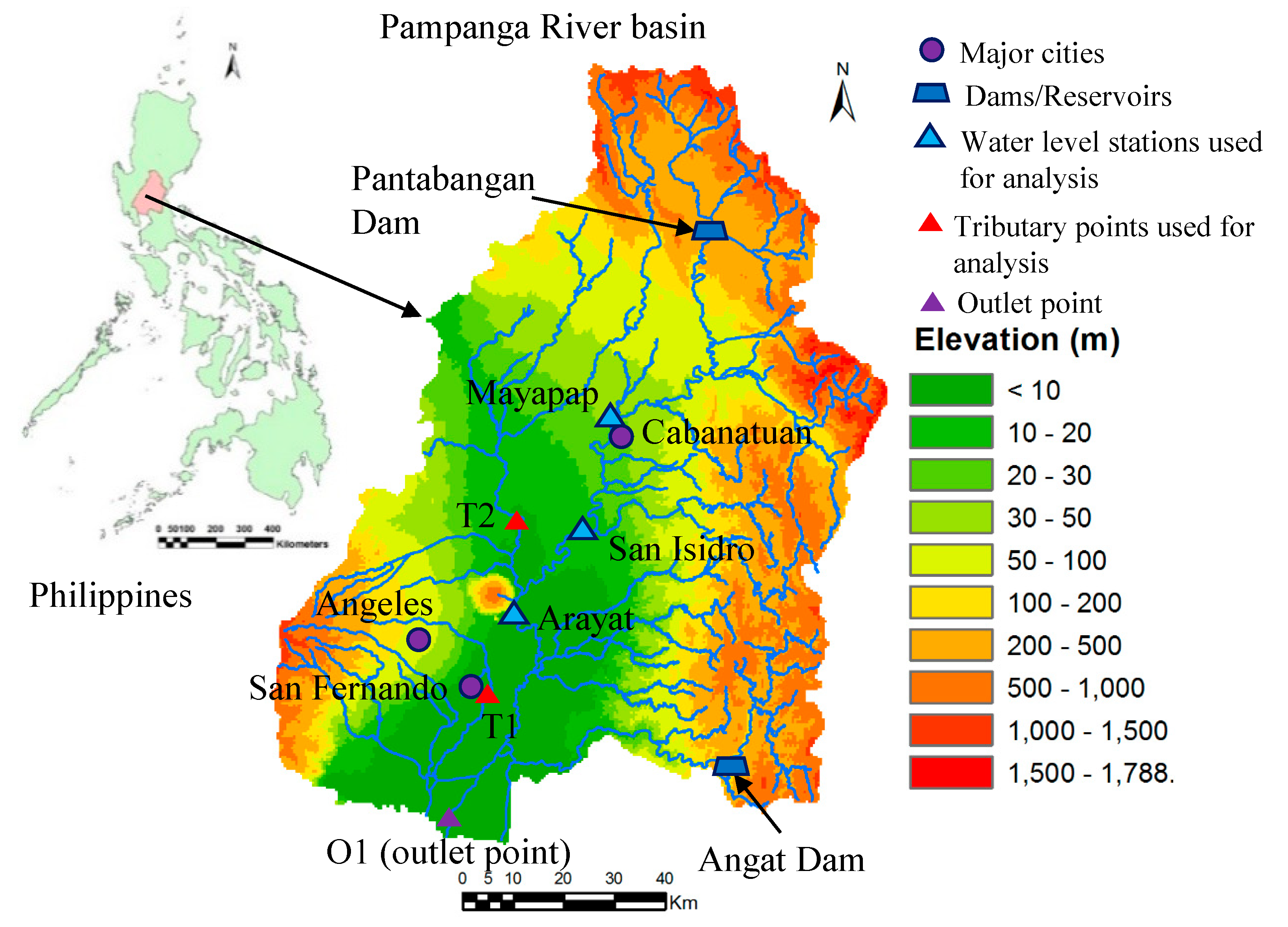
The Pampanga River basin, which is located in the Region III (Central Luzon) of the Philippines, is the fourth largest basin in the Philippines. Figure 2 shows the location map, basin boundary and digital elevation model (DEM) with elevation ranges of the study site. The catchment area of the study site is approximately 10,645 km2 (based on digital elevation model of study area) and the length of the main Pampanga River is about 260 km. About 95% basin area lies in Nueva Ecija, Tarlac, Pampanga, and Bulacan provinces of the Region III, while the remaining 5% area is part of the other seven provinces of the Region III such as Aurora, Zambales, Rizal, Quezon, Pangasinan, Bataan, and Nueva Vizcaya [15,16]. The average annual precipitation in the basin is 2155 mm [17]. There are two multi-purpose dams in the basin such as the Pantabangan dam (storage capacity of 2966 million m3) and Angat dam (storage capacity of 850 million m3). There are also two swamp areas in the river basin such as Candaba (250 km2) and San Antonio (120 km2) [17].
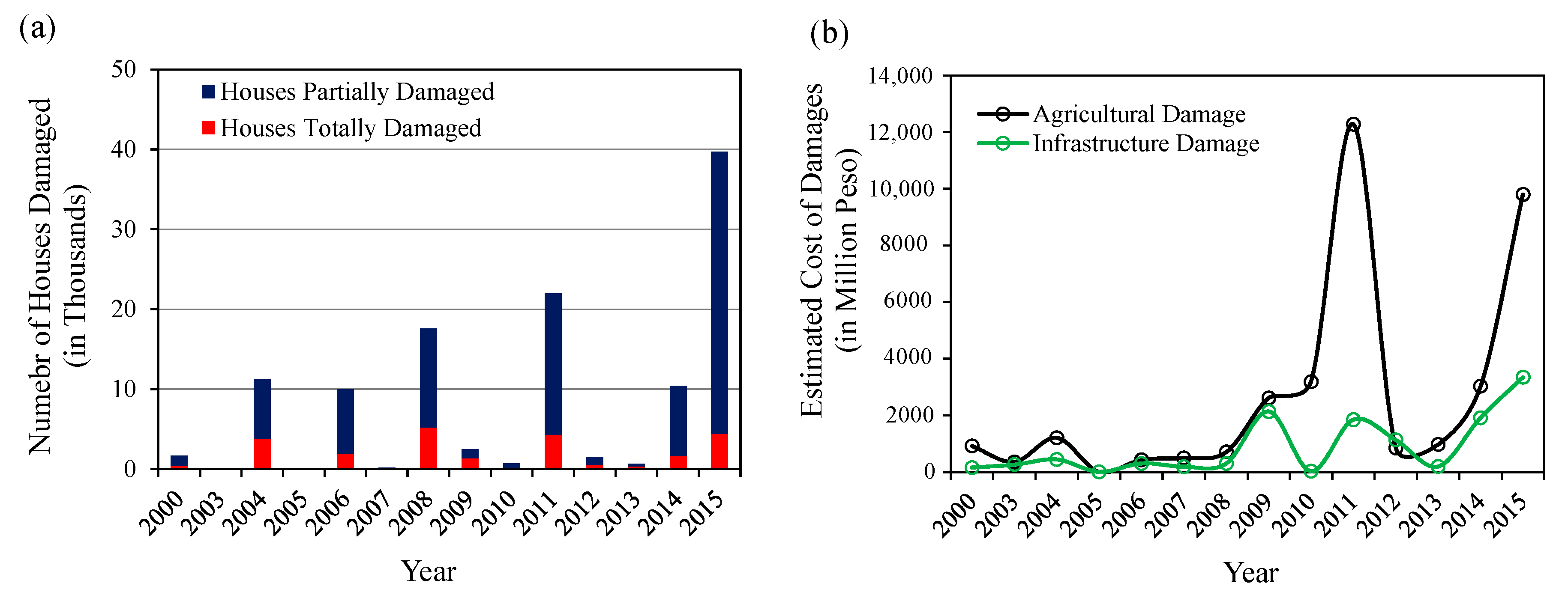
The population density in the study area in 2010 was 630 persons/km2 and the annual average population growth rate from 1980 to 2010 was about 2.61%, [17]. The cropland areas are widely spread over the central and downstream parts of the Pampanga River basin which are relatively flat and lowland areas, and built-up area is scattered in the basin [18]. However, the areas around three major cities such as San Fernando, Angeles and Cabanataun are continuously urbanized. This river basin is also regarded as one of the most important river basins in the Philippines since this basin makes an important contribution to the country’s economy [19]. On the other hand, this river basin experiences at least one flood event a year on average, which causes severe damage to house buildings, infrastructure, and agriculture in the basin [16]. Figure 3 shows the number of houses damaged by floods and the estimated value of flood damage to agriculture and infrastructures, in the Region III of the Philippines where study area is located. The figure shows the flood damage to houses, agriculture and infrastructure has been increasing in recent years. Therefore, it is necessary to analyze impact of continuous urbanization and land cover changes in the basin on flood runoff and inundations for proper adaptation measures and planning of land use to reduce the damage in future.
3. Data and Methodology
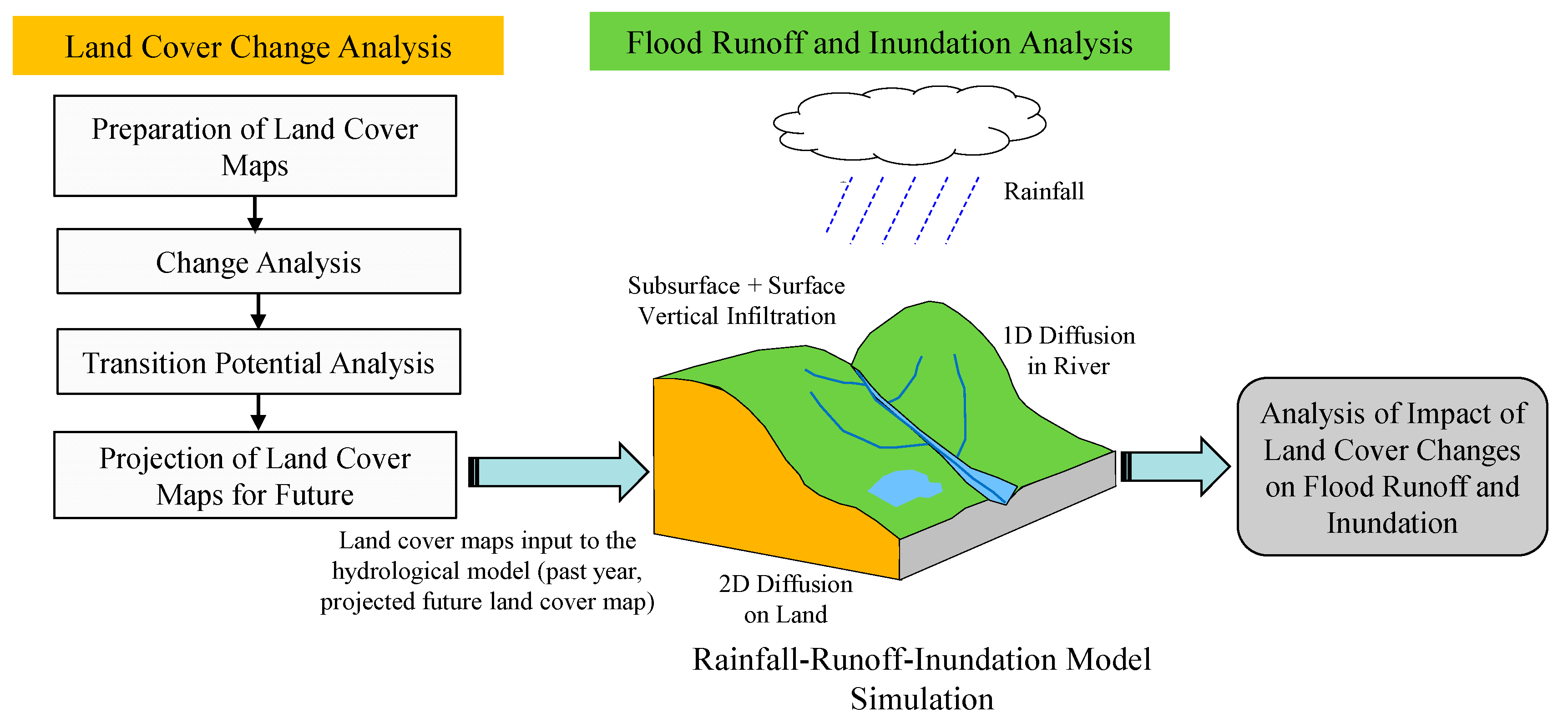
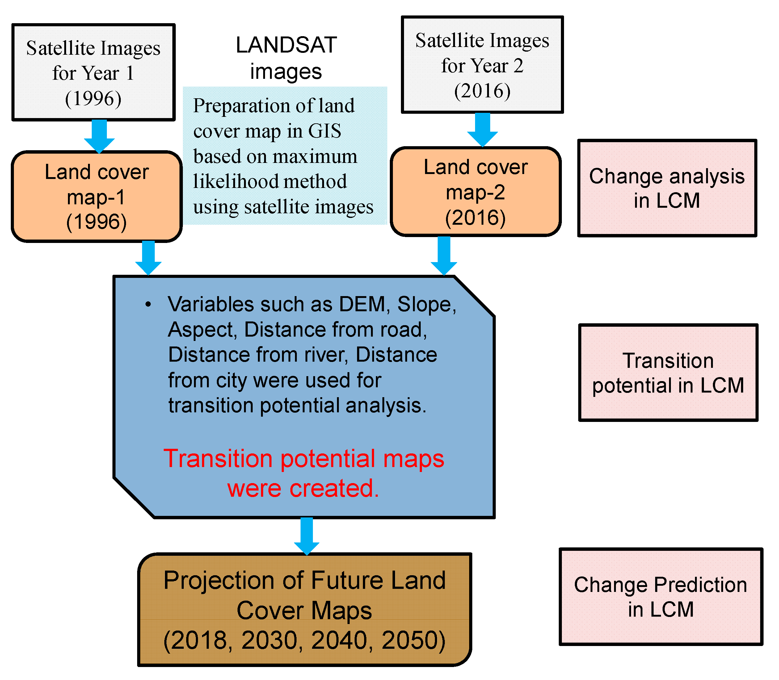
Figure 4 shows the overview of the research method. The research method includes two parts: (1) land-cover change analysis and projection for future, and (2) flood runoff and inundation analysis.
The land-cover maps for past years were generated using Landsat images based on supervised-maximum likelihood classification method and land cover changes in the past years were analyzed. The generated land-cover maps were validated by comparing these with Google Earth images. The land cover maps for the future were predicted using LCM based on the analysis of potential transition changes and considering various variables such as elevation, slope factors, aspect factors, distance from the city, distance from the major road, and distance from the river. Then, flood characteristics were analyzed using the RRI model developed by Sayama et al. [20] with land cover map for different years. The RRI model was calibrated and validated by comparing calculated flood discharge with observed discharge for past flood events, and calculated flood marks were also compared with recorded flood depth data. The impacts of land-cover changes on flood runoff, and flood inundation were analyzed for 50- and 100-year floods. The potential affected areas caused by flood hazards were also analyzed with different years land cover data. The details of methodology and data used are discussed below.
3.1. Land-Cover Change Analysis and Projection for Future
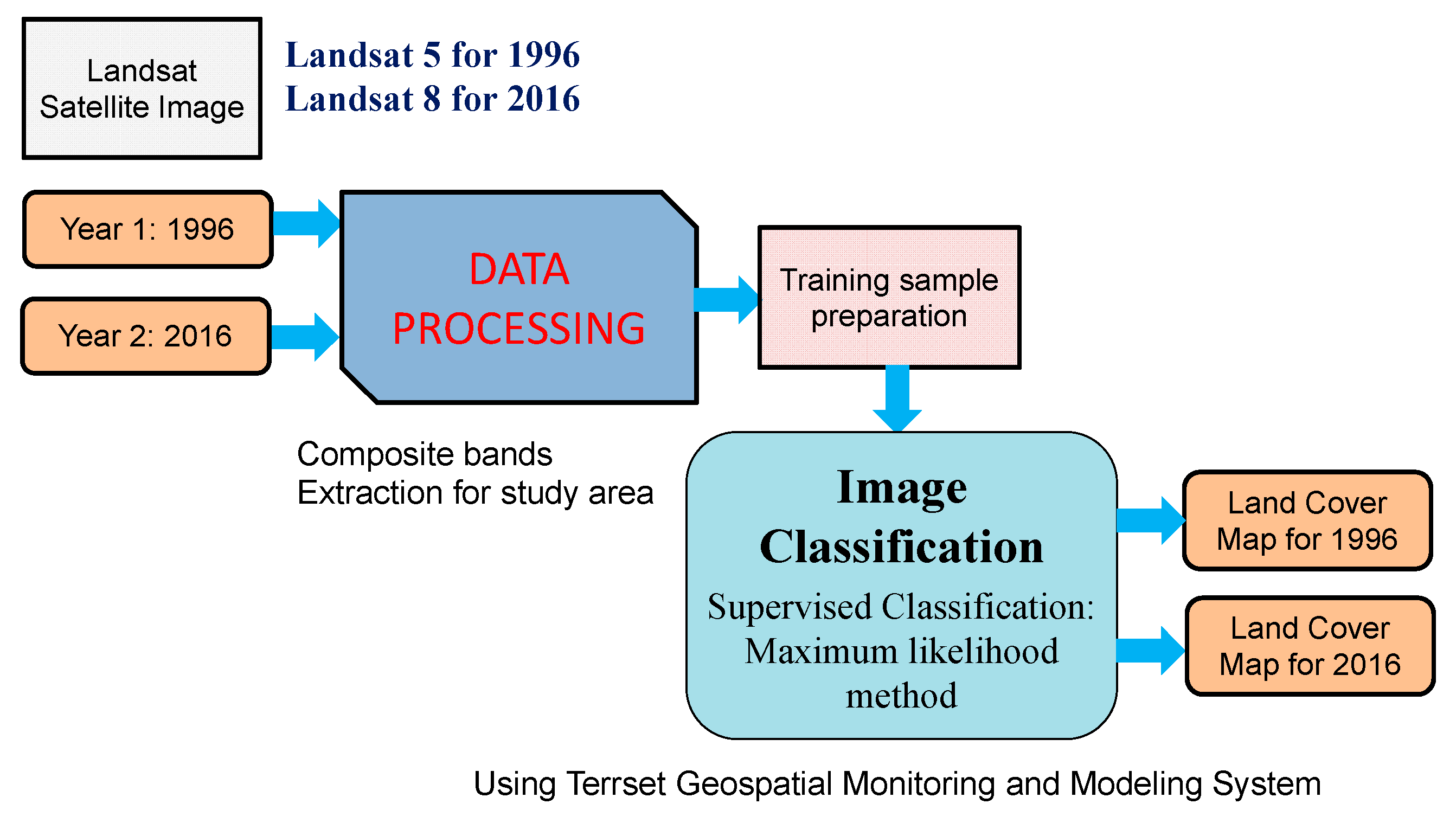
For land-cover change analysis, Landsat images were used because of their rich archive and spectral resolution [21]. In order to generate land-cover maps for past years, Landsat satellite images of 30m spatial resolution were acquired from the EarthExplorer database of United States Geological Survey with less than 10% cloud cover searching criteria for land cloud cover and scene cloud cover. Based on visual comparison of the images for cloud free or less cloud coverage images, Landsat 8 scenes acquired on 13 February 2016 for the year 2016 and Landsat 5 scenes acquired on 25 March 1996 for the year 1996 were selected for the land-cover classification in the study area. Pre-processing of the Landsat images were conducted using TerrSet Geospatial Monitoring and Modeling System (TGMMS). The raw digital number (DN) values of each band of the images were calibrated and converted to reflectance values, and the bands of the images were also corrected for atmospheric haze with dark object subtraction model in the TGMMS.
Figure 5 shows the overall process of generation of land-cover maps for past years. The composite band with combination of red, green and blue colors was created using the multiband of Landsat image for better visualization, which is very useful for making training samples. By using multiband, true color composite or false color composite can be created to represent an image. True color composite gives natural color to image with combination of red-green-blue (RGB) bands 321 in the case of Landsat 5 image and RGB bands 432 in the case of Landsat 8 image. False color composite gives color which is not natural with combination of RGB bands 432 in the case of Landsat 5 image and RGB bands 543 in the case of Landsat 8 image. These combinations of RGB bands in false color composite make vegetation and water in red and blue shades, respectively, which can be useful for the better visualization and identification of land areas and water bodies. In this study, both true color and false color composite images were prepared and used for making training samples.
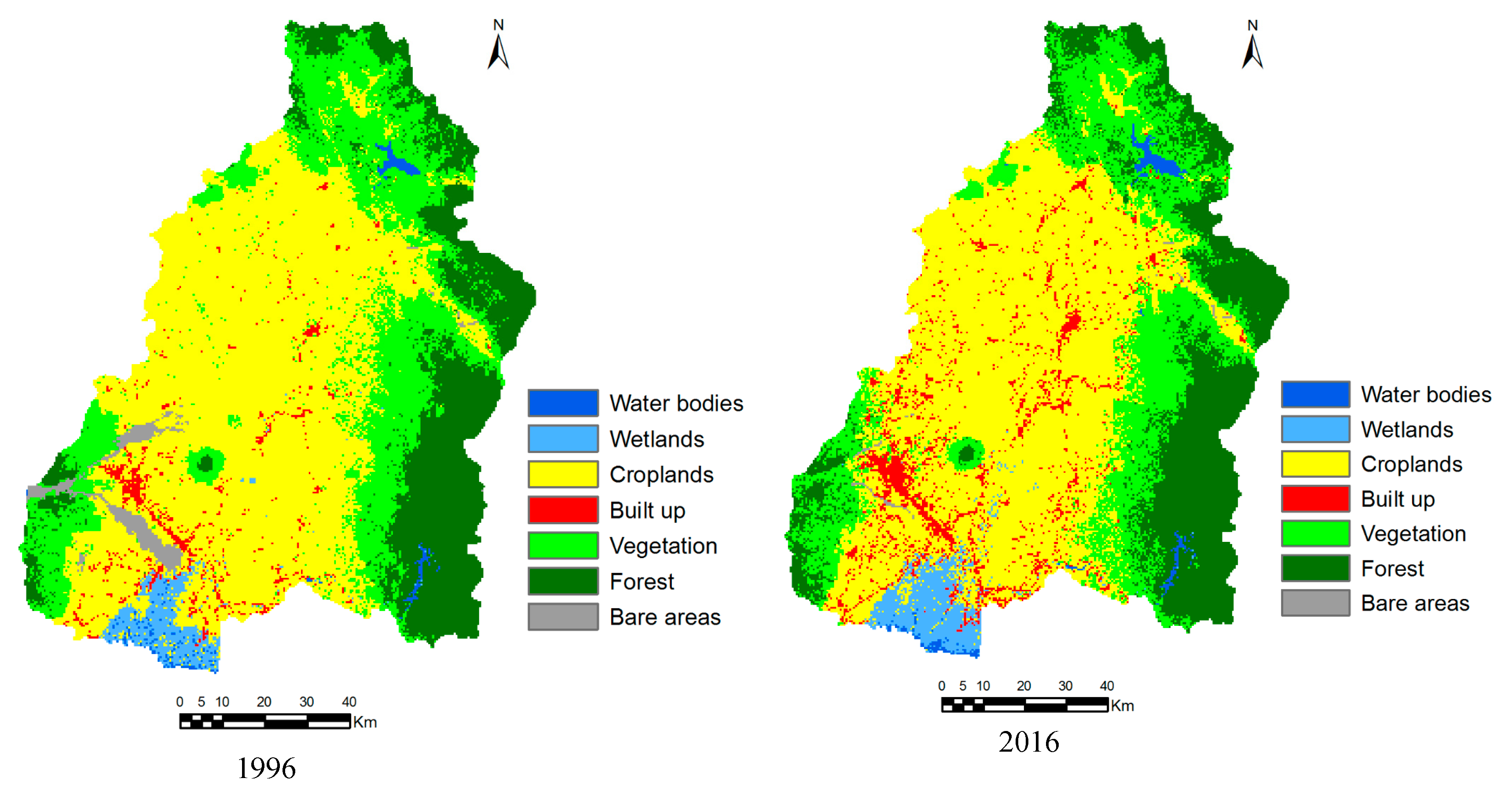
There are normally two methods of image classification, i.e., supervised and unsupervised classification. Supervised classification can generate desired classes of land-cover based on ground-truth data, while unsupervised classification attempts to classify the pixels with the same characteristics based on statistical criteria [21,22]. In this study, a supervised classification method was used, in which training samples and spectral signatures of known categories, such as urban, croplands, vegetation, forest and others, have to be developed. Then image classification tool in the TGMMS assigns each pixel in the image to the land-cover type to which its signature is most similar. The maximum likelihood classification method was used for image classification, which is one of the most effective algorithms for classification of satellite images [23,24]. The land-cover categories in the basin were classified into seven classes as presented in Table 1. The training samples for each land-cover class for 1996 and 2016 were selected as many as possible throughout the entire image based on composite images as well as google earth images. About 672 training samples (water bodies: 49, wetlands: 70, cropland: 330, built-up areas: 114, vegetation: 58, forest: 22, bare land: 29) were selected for land-cover class for 1996, while about 1128 training samples (water bodies: 99, wetlands: 103, cropland: 552, built-up areas: 245, vegetation: 80, forest: 30, bare land: 19) were selected in the case of 2016 (Table 1). After making training samples for 1996 and 2016, signature files were created by processing Band 1 to Band 6 using the IDRISI image processing tool in the TGMMS. Then, by using signature files, land cover maps for the years 1996 and 2016 were generated based on maximum likelihood classification method. The generated land-cover maps of 30m spatial resolution were upscaled to 450m spatial resolution, same as spatial resolution of DEM used for hydrological analysis, using ArcGIS 10.3.1 (Esri, Redlands, CA, USA). The generated land-cover maps were compared visually with google earth images. For the fully or partly could coverage areas, generated maps were manually corrected based on Google Earth images using raster editor in ArcGIS 10.3.1 (Redlands, California). Figure 6 shows the generated land cover maps for the years 1996 and 2016. The accuracy assessment of generated land cover maps was also performed by checking random samples of land cover class with google earth images. The overall accuracy and kappa value for 1996 land cover were about 87.3% and 0.806, while they were about 86.5% and 0.801 in the case of 2016 land-cover map. The generated land cover maps for the years 1996 and 2016 were in perfect agreement with high value of overall accuracy and kappa value. The land-cover maps show that the cropland and built-up areas were mostly located in the region with 0–50 m altitude and a slope of 0–5 degrees. The vegetation and forest areas were densely located in the region where the altitude is greater than 200 m. The wetlands areas were mostly located in the coastal areas where water covers the land throughout the year because of the effect of sea/tidal level.
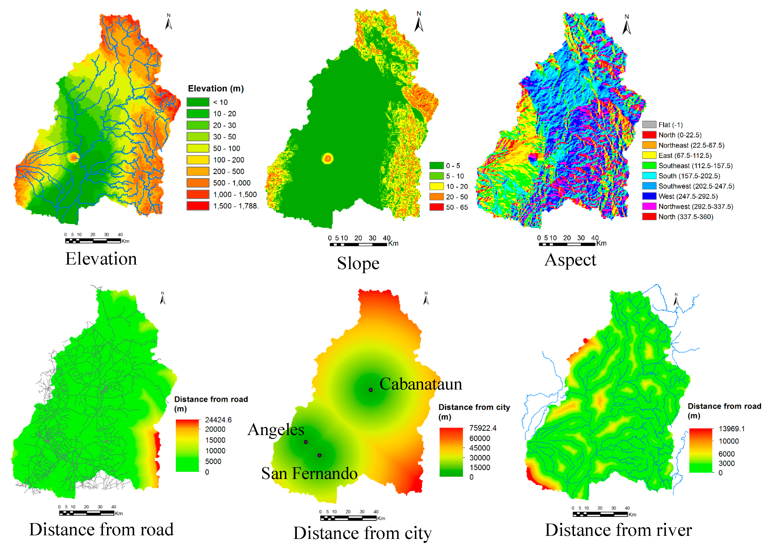
Figure 7 shows the process of land cover change analysis, transition potential analysis and prediction of land cover maps for the future. To predict land cover maps for future years, land cover changes between the years 1996 and 2016 were analyzed using the LCM tool of TGMMS. The potential for land transitions was modeled using transition sub-model of LCM with similarity-weighted instance-based machine learning tool (SimWeight) [25]. Six transitions such as cropland to built-up, cropland to vegetation, vegetation to cropland, vegetation to built-up, vegetation to forest, and forest to vegetation, were considered for potential transition modeling. The changes in water bodies, wetlands and bare areas were neglected for future projection of land-cover maps. The variables such as elevation, slope, aspect, distance from the road, distance from the city centre, and distance from the river as shown in Figure 8 were also considered as static variables in the potential transition modeling. Then, land-cover maps were predicted for years 2018, 2030, 2040 and 2050 based on historical rates of change and the transition potential model. The projected land-cover map for year 2018 was used only for validation of the projected map, and the land-cover maps for years 2030, 2040, and 2050 were used for impact analysis of land cover changes on flooding regime. The land use plan of local governments was not considered in prediction of land-cover maps for future dates, because of limited information and data. The LCM tool of TGMMS can predict a future scenario of land cover for a specified future year based on the historical rates of change and the transition potential modeling [26]. The LCM model determines how the variables influence land cover change in the future, how much land-cover change took place between year 1 and year 2, and then calculate a relative amount of transition to the future year [26].
3.2. Flood Hazard Assessment and Impact Analysis
Many rainfall-runoff models, such as HEC-HMS [27], TOPMODEL [28], Tank model [29] and others, which have been applied for runoff prediction, cannot compute flood inundation. Therefore, the RRI model, developed by Sayama et al. [20], was employed to simulate flood characteristics such as flood runoff, inundation depth, flood duration and extent areas. The RRI model is also available for free. The RRI model is a two-dimensional hydrological model, which can simulate rainfall-runoff process, infiltration process and flood inundation simultaneously [20]. The RRI model simulates flow characteristics in the slopes and river channels separately. The flow on the slope grid cells is calculated with a two-dimensional diffusive wave model, while the flow on the river channel is calculated with a one-dimensional diffusive wave model. The details on the governing equations of the RRI model can be found in Sayama et al. [20]. The Interferometric Synthetic Aperture Radar (IfSAR) acquired in 2013 was obtained from the National Mapping and Resource Information Authority (NAMRIA) of the Philippines. A DEM of 15 arc-s (approximately 450 m horizontal resolution), derived from the IfSAR, was used in the RRI model simulation. The river width and depth were calculated at each river grid cell using empirical equations [20]. The constant values of the empirical equations were estimated based on measured cross-sectional information and google earth images at several locations. Based on the past dam release discharge data obtained from the Pantabangan and Angat Dam offices, the Pantabangan dam generally stores all the inflow discharges during the flood event, while the Angat dam mostly releases the discharge during a flood event [30]. Therefore, the flood control function of only Pantabangan dam was considered in the analysis. It was assumed that no outflow from the dam was considered until the flood control storage capacity is filled up (flood storage capacity of the Pantabangan dam is about 1018 million m3), and when the flood storage volume of the dam exceeds the capacity, the outflow discharge from the dam was considered to be the same as the inflow discharge. The ground gauge rainfall data at 17 stations were used and Thiessen polygon method was employed for the spatial distribution of rainfall in the basin. The recent largest flood events i.e. 2011 flood and 2015 flood, were selected for model calibration and validation. The parameters of RRI model were calibrated with September 2011 flood event by comparing calculated discharge with observed data. The results of calculated flood inundation depth were also compared with the recorded flood mark data. The calibrated parameters of the model were validated with October 2015 flood event.
In general, flood risk assessment is conducted for a specific return period flood event or for the recorded past largest flood event [31]. The target scale of flood risk assessment varies by river according to socio-economic activities, past disasters, and expected damage in the basin [31]. In this study, flood hazard assessment was conducted by using RRI model for 50- and 100-year flood cases using past years land cover data (1996 and 2016) and also using predicted future land-cover maps for 2030, 2040 and 2050. Statistical analysis was conducted using 48-hours maximum annual precipitation to estimate rainfall intensity for different return periods. Spatial and temporal rainfall distribution of September 2011 flood were selected to design rainfall hyetograph for different return periods, and it was estimated by multiplying the rainfall of September 2011 flood event by a rainfall conversion factor. The rainfall conversion factor for each return period can be estimated as the ratio of the corresponding rainfall volume of the return period and the rainfall volume of September 2011 [30,31]. Flood hazard was simulated using RRI model with rainfall hyetograph of different return periods considering different years land cover map.
4. Results and Discussions
4.1. Results of Land-Cover Change Analysis and Projection for Future
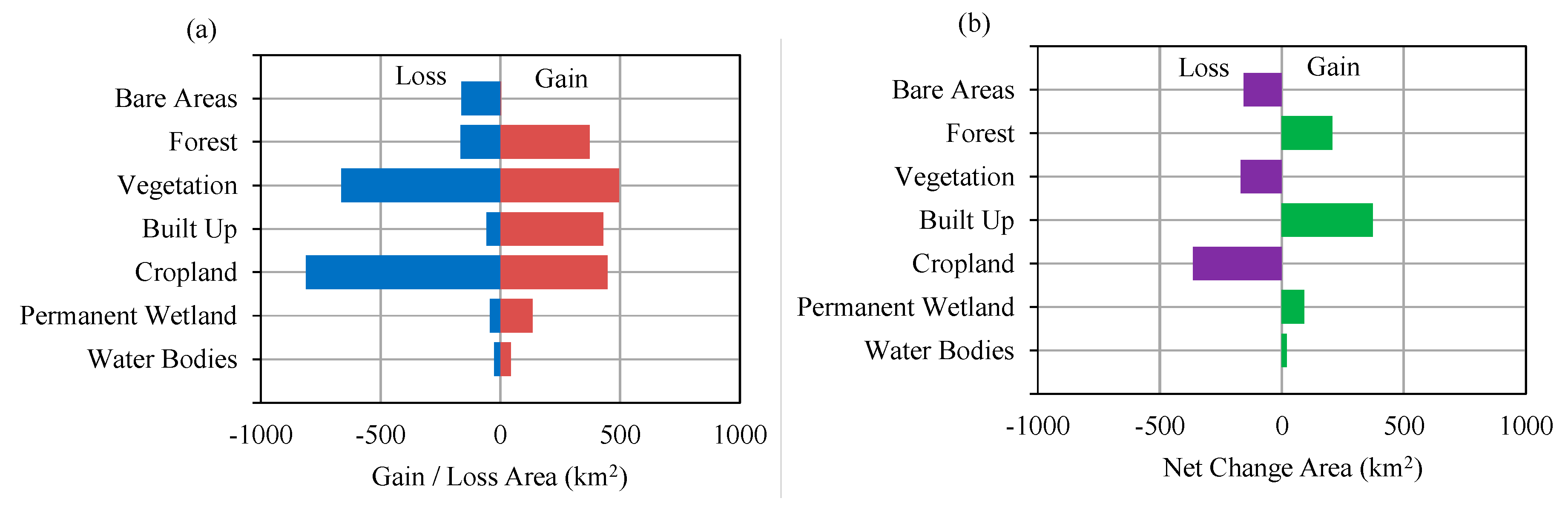
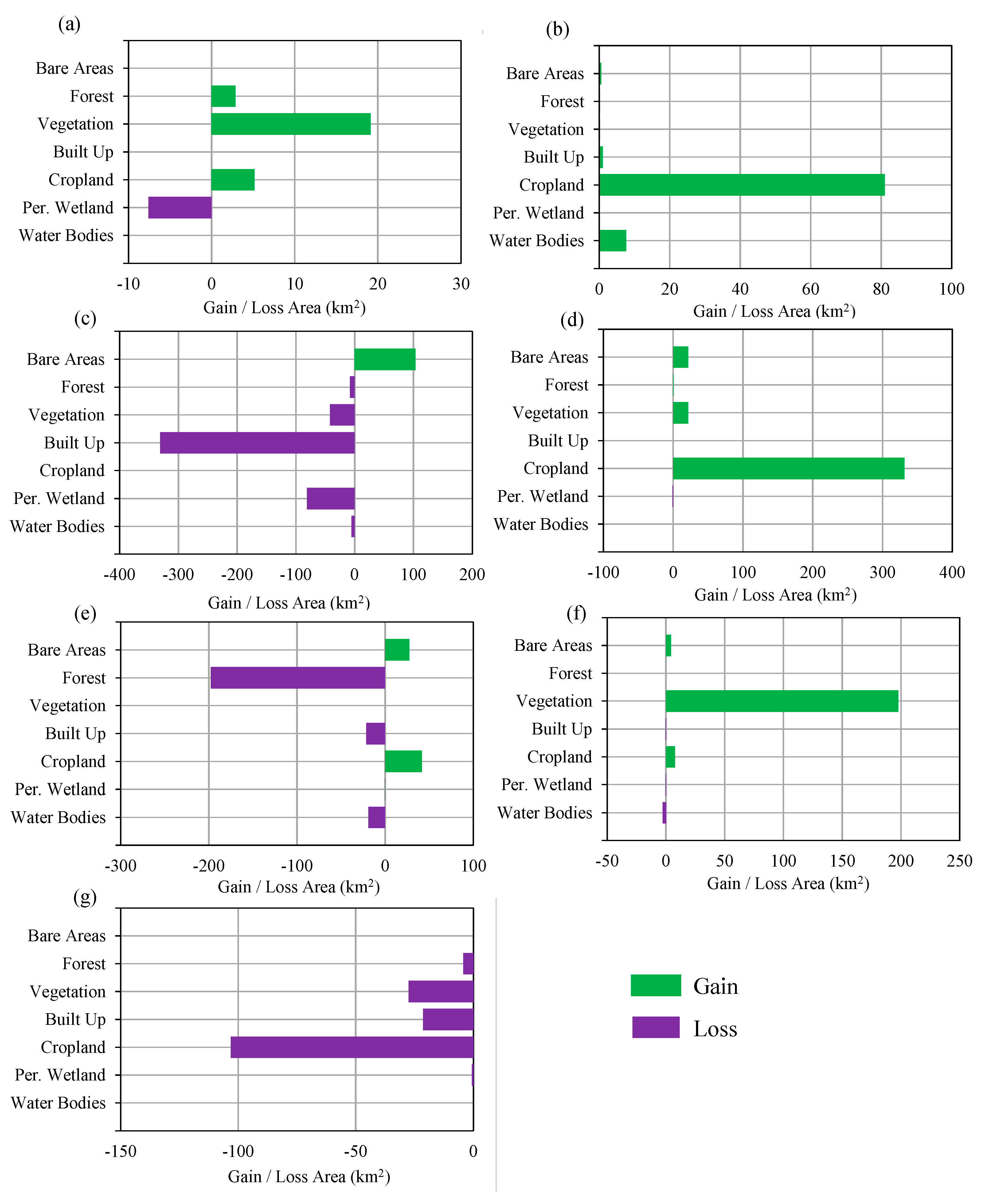
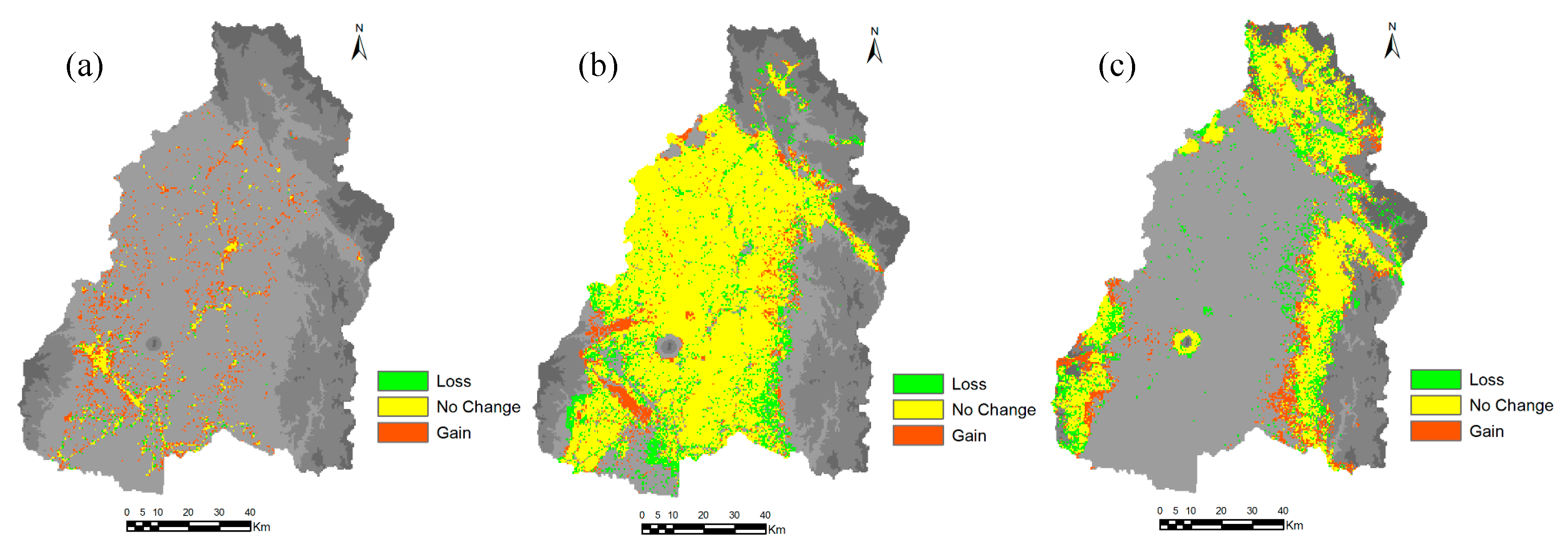
Table 2 shows the area of each land cover class in 1996, 2016, 2030, 2040, and 2050. In 1996, the study area was largely dominated by croplands (5488.67 km2), about 51.5% of the total area. The built-up areas were about 227.34 km2 (2.14% of the study area). In 2016, the cropland areas decreased to 5125.07 km2 (48.14% of the study area) and built-up areas increased to 600.4 km2 (5.64% of study area). Figure 9 shows the gain/loss area and net change area of land cover between 1996 and 2016. The figure shows that cropland, vegetation and bare areas decreased from 1996 to 2016, while other areas increased. Figure 10 shows the contribution to net change from 1996 to 2016 for each land-cover class and Figure 11 shows the distribution of loss, no change and gain areas in the case of built-up, cropland and vegetation land-cover classes. The results show that areas gain in water bodies were from the forest, vegetation and cropland, particularly in the upstream of dams. The loss areas of water bodies were mainly converted to wetland, particularly in coastal areas. The gain of permanent wetland areas was mainly from the cropland. Some cropland areas were used for fishponds in recent years and also some areas located in coastal areas become wet throughout the year. The contribution to net change in cropland shows that cropland areas were mainly converted to built-up area. The land-cover maps of 1996 and 2016 shows that the built-up areas were scattered in the large areas. However, the areas around San Fernando, Angeles and Cabanatuan were largely urbanized in 2016 compared to the year 1996. The gain of built-up area was mainly from cropland and some from bare areas and vegetation. The croplands areas are mostly located in the low-lying areas where built-up areas can be easily expanded. Vegetation areas were mainly converted to forest areas. The bare areas, particularly which was created by Mt. Pinatubo eruption in 1991, were converted mainly to cropland, built-up and vegetation.
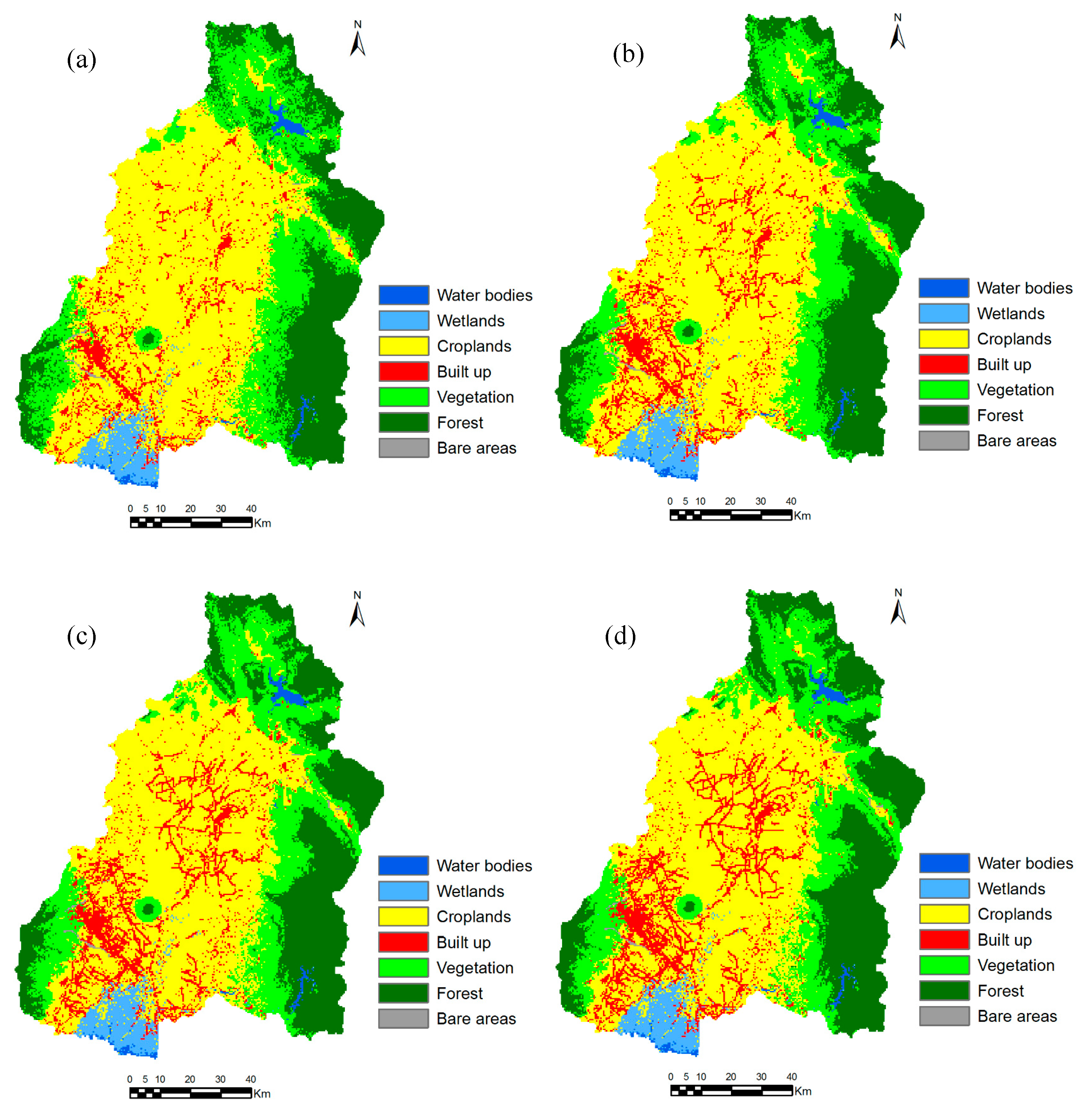
Figure 12 shows the projected land-cover map for years 2018, 2030, 2040 and 2050. The projected land-cover map for 2018 was compared visually with Google Earth image of February 2018. The random samples of land-cover class were also generated in Geographic Information System (GIS), and the Keyhole Markup Language (KML) data of random samples were imported into Google Earth for comparison. The overall accuracy and kappa value in the case of projected land cover map of 2018 were about 90.4% and 0.858, which were in perfect agreement.
The comparison of past and projected land-cover maps shows that the croplands and vegetation areas are decreasing in trend, while built-up and forest areas are increasing in trend (Table 2, Figure 12). The projected maps also show that the built-up areas are largely increasing around San Fernando, Angeles and Cabanatuan as well as along the roads. The comparison of net change of land cover map between 2016 and 2050 shows that cropland areas and vegetation may decrease in 2050 by 11.25% and 9.3%, respectively. The built-up areas and forest areas may increase in 2050 by 93.2% and 10.6%, respectively.
4.2. Results of Flood Impact Analysis
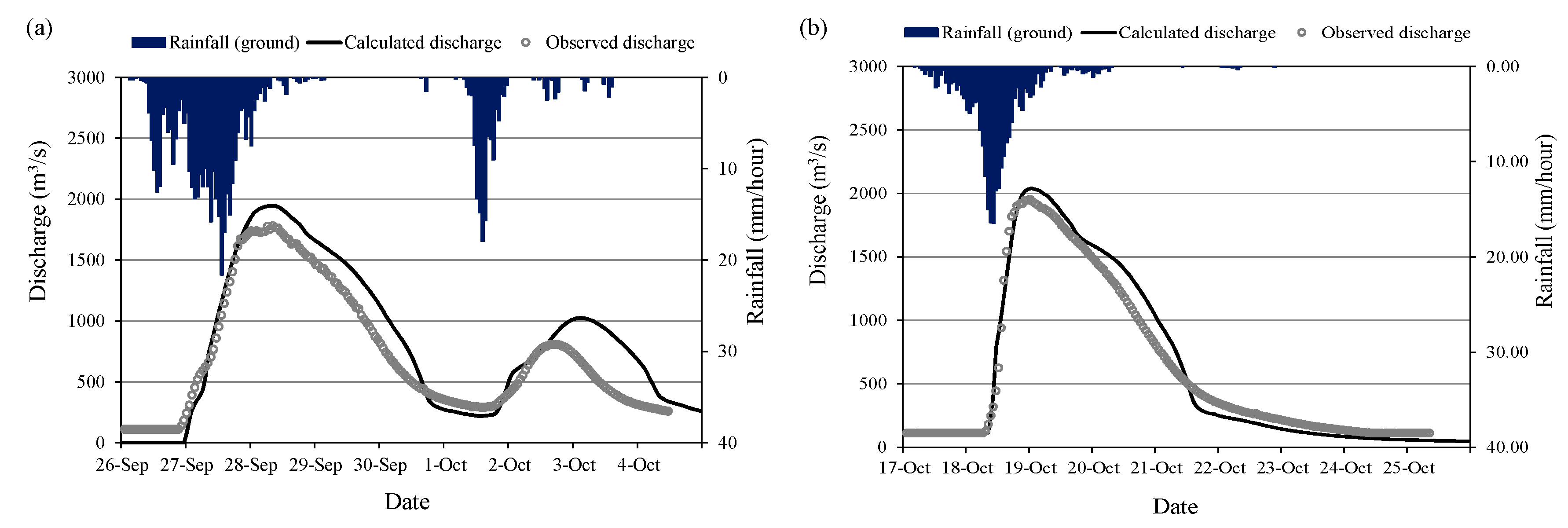
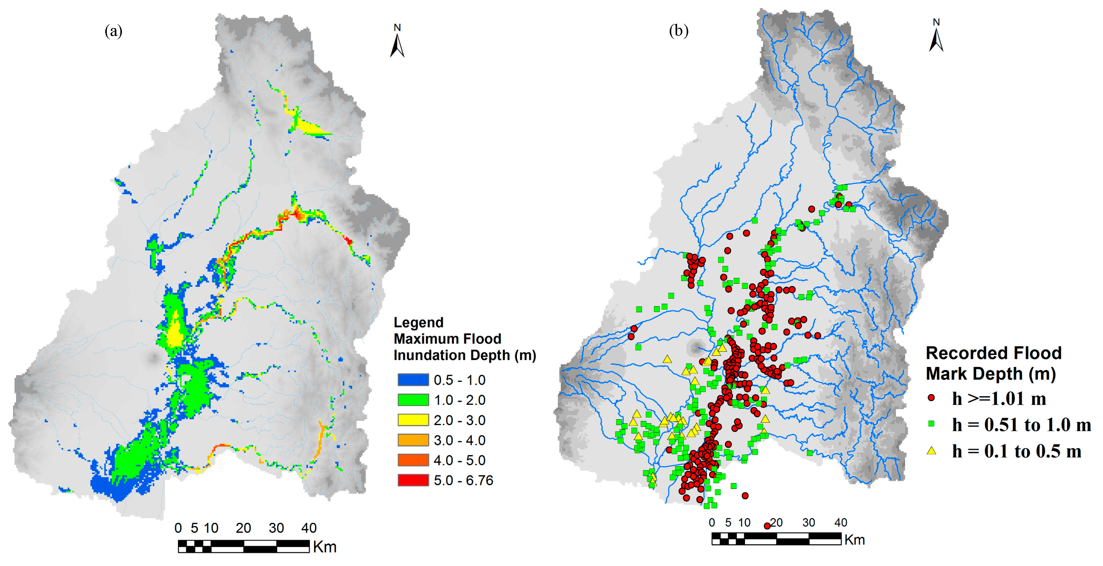
Figure 13 shows the comparison of calculated discharge using RRI model at San Isidro station with observed discharge for 2011 flood and 2015 flood events. The 2011 flood event was used for RRI model calibration and the 2015 flood event was used for validation of the calibrated parameters. The land cover map of 2016 was used for both flood event cases for the simplicity. The model parameters were calibrated with 2011 flood using 2016 land cover map; however, the calibrated parameters of the model were also confirmed/validated with 2015 flood event using the same land cover map of 2016. The values of R2 (squared of correlation coefficient) and Nash Sutcliff Coefficient of Efficiency (NSCE), which are commonly used metrics for evaluation of the model performance in hydrology, were 0.91 and 0.82 in the case of discharge at San Isidro for 2011 flood, while 0.82 and 0.8 for 2015 flood. The calculated discharge at the San Isidro station matches well with the observations indicating high R2 and NSCE values. The results of calculated flood inundation depth were also compared with recorded flood mark depth at the selected locations as shown in Figure 14. The red circle points in the Figure 14b show the areas of recorded flood depth greater than 1.01 m [32]. The green rectangle and yellow triangle points in the figure show the areas of recorded flood depth ranges from 0.51–1.0 m and less than 0.5, respectively. The calculated flood extent areas and depth trends are similar to the recorded flood mark data.
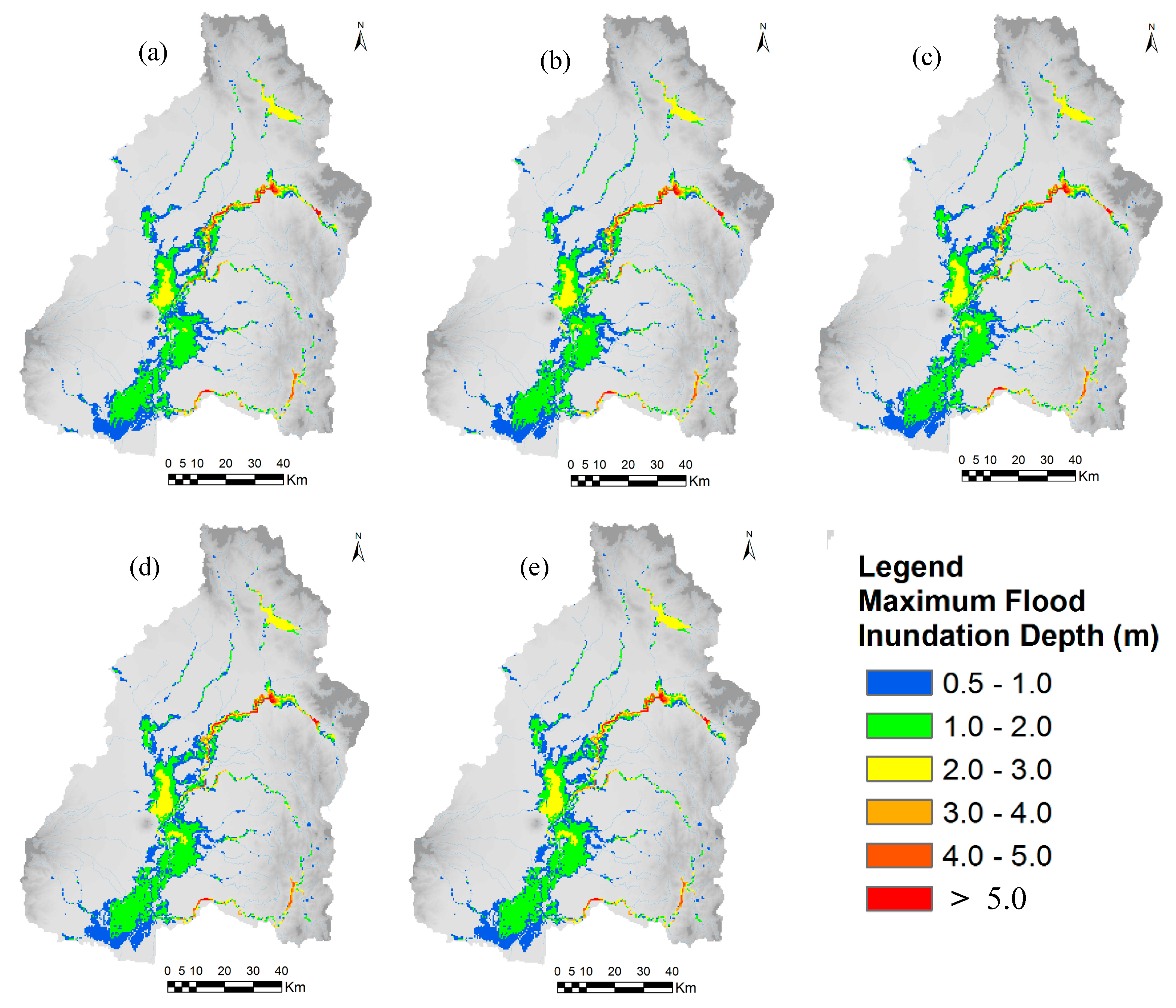
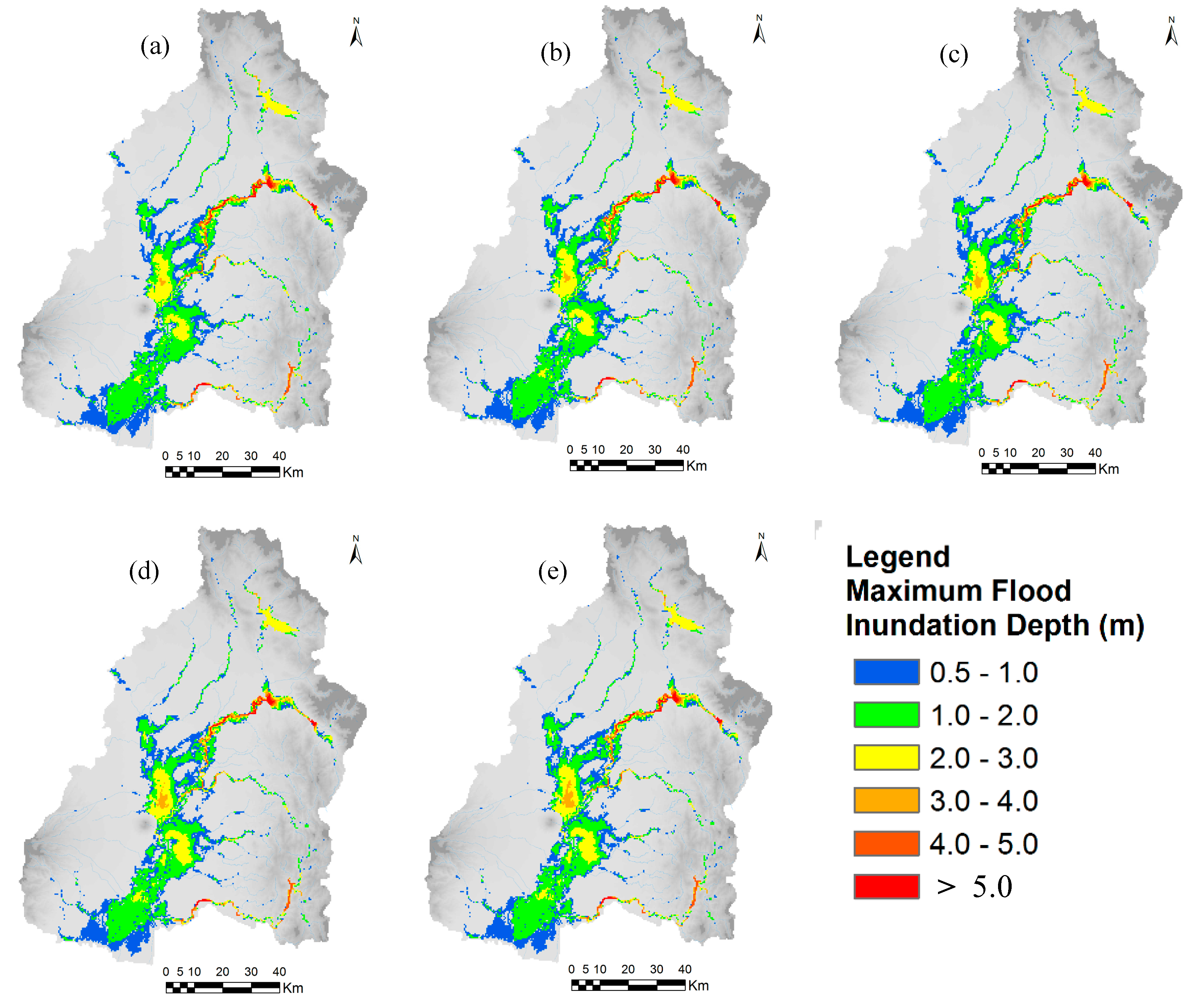
The annual maximum 48-hours rainfall of September 2011 flood was about 299.011 mm, and the values of 48-hours rainfall for 50-year flood and 100-year flood based on frequency analysis, were about 330 mm and 369 mm, respectively. The rainfall hyetographs for 50- and 100-year return periods were estimated by multiplying the rainfall pattern of September 2011 flood event by a rainfall conversion factor. Figure 15 and Figure 16 show the calculated flood inundation depth and extent areas with different year land-cover maps (1996, 2016, 2030, 2040, and 2050) in the cases of 50- and 100-year floods, respectively. The results show that flood inundation depth and flood extent areas are increasing in trend in the middle and lower areas of the basin due to land-cover changes, mainly due to rapid urbanization of three main cities such as San Fernando, Angeles and Cabanataun, and also expanding built-up areas along the road networks. The flood inundation depth and flood extent areas may increase in the future due to urbanization activities and conversions of croplands into built-up areas. Urbanization and growing of built-up areas can cause a large amount of pervious areas to change into impervious areas by reducing infiltration rates which results increase in runoff.
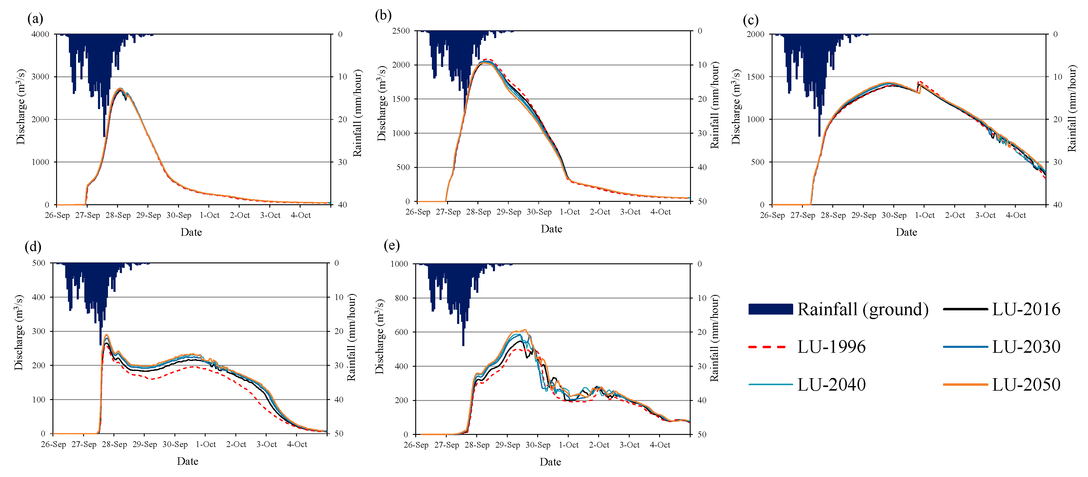
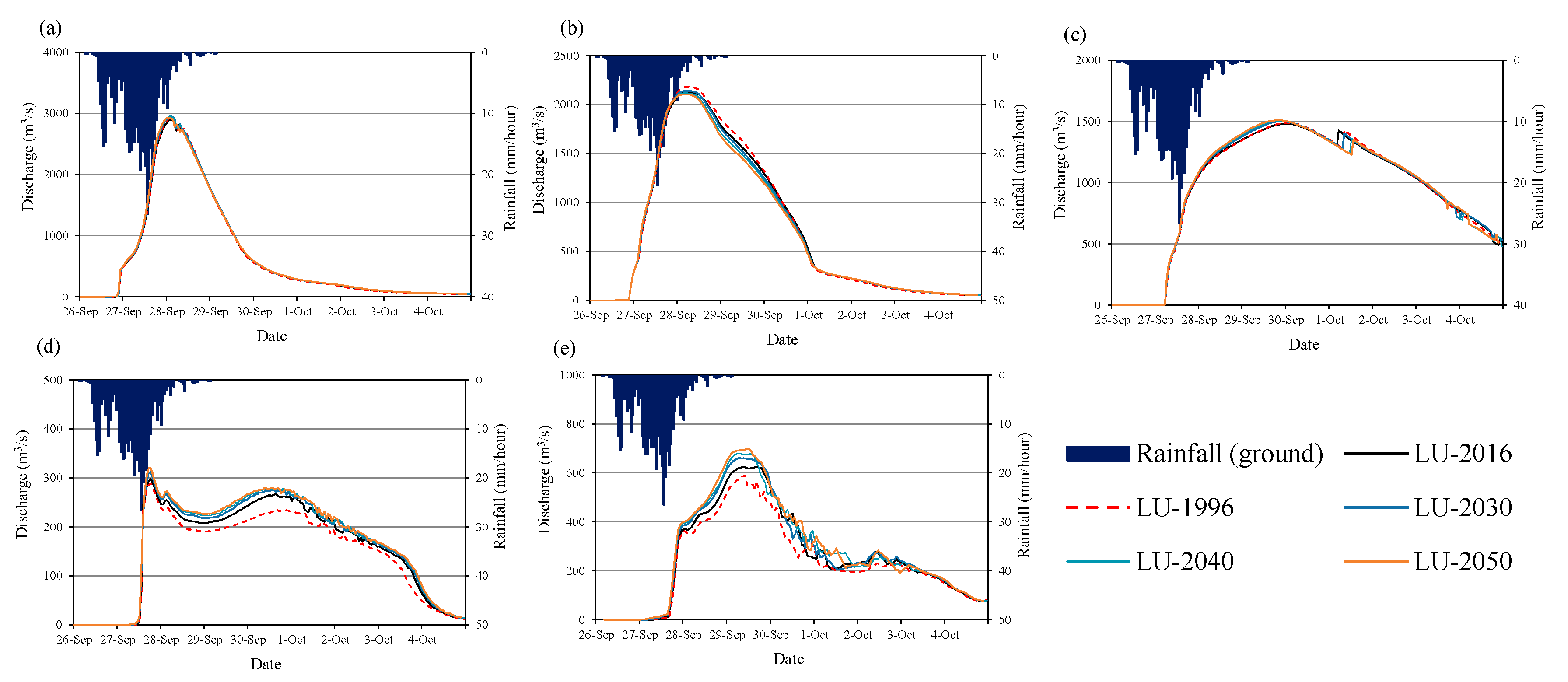
Figure 17 and Figure 18 show the change in flow discharge with different years land cover at Mayapap, San Isidro, Arayat, and tributary rivers (T1 and T2), respectively (see Figure 2 for the locations of these points). The results show that the river runoff may increase in the future due to land-cover changes and urbanization activities, particularly in the middle and downstream reach of the basin. The changes in the river discharge due to land-cover change are significantly higher at tributaries compared to the main river channel.
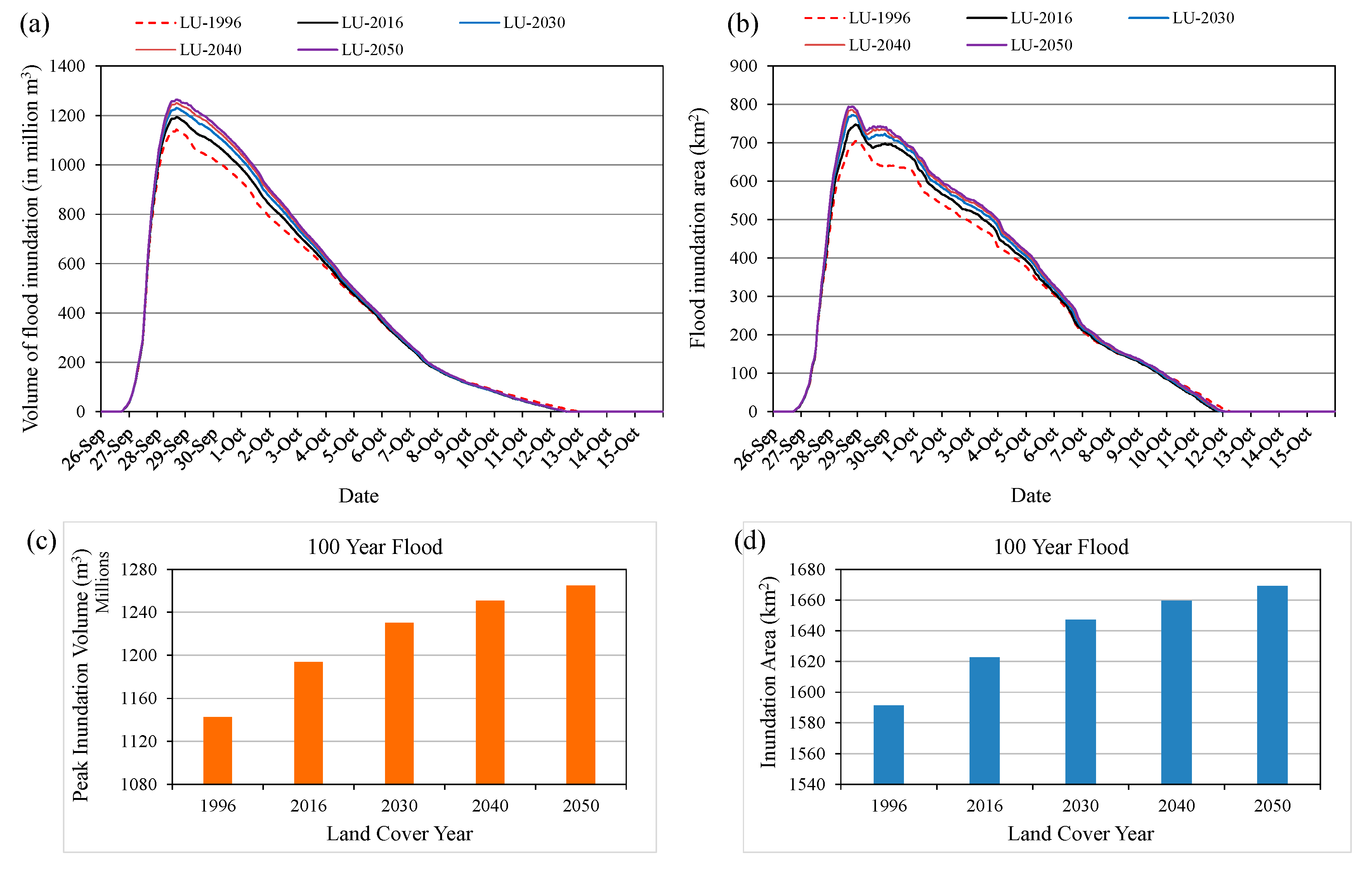
Figure 19a,b show the temporal changes in flood inundation volume and flood extent areas with different year land-cover data in the case of 100-year flood. Figure 19c shows the peak value of flood inundation volume, and the total flood extent areas during the flood event are presented in Figure 19d. The results show that flood inundation volume, peak value of flood volume and flood extent areas may increase in the future due to land-cover changes, particularly due to rapid urbanization of three main cities and expansion of built-up areas along the roads by converting cropland and vegetation areas into built-up areas. The peak value of flood inundation volume and total flood extent areas in the case of using 1996 land-cover map were found to be 1142 million m3 and 1591 km2 respectively, while 1265 million m3 and 1669 km2 in the case of using 2050 land cover map. The flood impact in the basin may increase in the future due to land cover changes and urbanization activities. The cropland areas and fishpond areas are mostly located in low land areas of the basin, where flood impact might be greater in the future.
5. Conclusions
The land-use/land-cover changes and their impact on flood runoff, flood hazards and inundation were analyzed in the Pampanga River basin of the Philippines. The land-use/land-cover changes were analyzed between 1996 and 2016 using Landsat images and image processing tools in GIS, and the land-cover maps for future years were projected. The main changes observed for the time period of 1996–2016 were cropland and built-up areas. The cropland areas in the basin decreased by approximately 358.03 km2 from 1996 to 2016, and built-up areas increased by approximately 367.3 km2. The vegetation areas decreased by approximately 166.32 km2 and forest areas increased by approximately 203.27 km2. The bare land areas also decreased by approximately 154.76 km2. The cropland areas in the basin were mainly converted to built-up area, and vegetation areas were mainly converted to the forest area. The bare areas were mainly converted to cropland, built-up and vegetation. The result of land-cover changes between 2016-2050 shows that the crop land area and vegetation may decrease in 2050 by 11.25% and 9.3%. The built-up areas and forest areas may increase in 2050 by 93.2% and 10.6%.
Flood inundation depth and flood extent areas are increasing in trend in the middle and lower areas of the basin due to land-cover changes, which is mainly due to rapid urbanization of three main cities San Fernando, Angeles and Cabanatuan as well as expansion of built-up areas along the road networks. The flood inundation depth and flood extent areas may increase in the future due to urbanization activities and conversions of cropland into built-up areas. The changes in river discharge due to land-cover change are significantly higher at tributaries compared to the main river channel. The flood inundation volume and flood extent areas may also increase in the future. The results obtained in this study can be useful for proper planning and management of land use in the basin, and also it will be useful to reduce the risk of flood in the future. The flood runoff and inundation analysis considering land-cover change provides useful information for better understanding of land-use/land-cover impacts. In this study, land use plan of local government was not considered for projection of land-cover map for future. If such a plan is available, it is recommended to consider it in further study. The variables such as elevation, slope factors, aspect factors, distance from the city, distance from the major road, and distance from the river, were considered as static variables for future projection of land-cover maps. The dynamic changes of such variables, particularly existing the plan of the future expansion of the road, are also recommended to consider in a further study.
Funding
This research received no external funding.
Acknowledgments
The author would like to acknowledge to the all related counterpart organizations for providing data.
Conflicts of Interest
The authors declare no conflict of interest.
References
- Ranger, N.; Hallegatte, S.; Bhattacharya, S.; Bachu, M.; Priya, S.; Dhore, K.; Rafique, F.; Mathur, P.; Naville, N.; Henriet, F.; et al. An assessment of the potential impact of climate change on flood risk in Mumbai. Clim. Chang. 2011, 104, 139–167. [Google Scholar] [CrossRef]
- Blöschl, G.; Ardoin-Bardin, S.; Bonell, M.; Dorninger, M.; Goodrich, D.; Gutknecht, D.; Matamoros, D.; Merz, B.; Shand, P.; Szolgay, J. At what scales do climate variability and land cover change impact on flooding and low flows? Hydrol. Process. 2007, 21, 1241–1247. [Google Scholar] [CrossRef]
- Apollonio, C.; Balacco, G.; Novelli, A.; Tarantino, E.; Piccinni, A.F. Land use change impact on flooding areas: The case study of Cervaro basin (Italy). Sustainability 2016, 8, 996. [Google Scholar] [CrossRef]
- Iwami, Y.; Hasegawa, A.; Miyamoto, M.; Kudo, S.; Yusuke, Y.; Ushiyama, T.; Koike, T. Comparative study on climate change impact on precipitation and floods in Asian river basins. Hydrol. Res. Lett. 2017, 11, 24–30. [Google Scholar] [CrossRef] [Green Version]
- Loo, Y.Y.; Billa, L.; Singh, A. Effect of climate change on seasonal monsoon in Asia and its impact on the variability of monsoon rainfall in Southeast Asia. Geosci. Front. 2015, 6, 817–823. [Google Scholar] [CrossRef] [Green Version]
- Detrembleur, S.; Stilmant, F.; Dewals, B.; Erpicum, S.; Archambeau, P.; Pirotton, M. Impacts of climate change on future flood damage on the river Meuse, with a distributed uncertainty analysis. Nat. Hazards 2015, 77, 1533–1549. [Google Scholar] [CrossRef] [Green Version]
- Kimaro, T.A.; Tashikawa, Y.; Takara, K. Distributed hydrologic simulations to analyze the impacts of land use changes on flood characteristics in the Yasu River basin in Japan. J. Nat. Disaster Sci. 2005, 27, 85–94. [Google Scholar]
- Amini, A.; Ali, M.A.; Ghazali, A.H.B.; Aziz, A.A.; Akib, S.M. Impacts of land-use change on streamflows in the Damansara watershed, Malaysia. Arab. J. Sci. Eng. 2011, 36, 713–720. [Google Scholar] [CrossRef]
- Yulianto, F.; Prasasti, I.; Pasaribu, J.M.; Fitriana, H.L.; Zylshal; Haryani, N.S.; Sofan, P. The dynamics of land use/land cover change modeling and their implications for the flood damage assessment in the Tondano watershed, North Sulawesi, Indonesia. Model. Earth Syst. Environ. 2016, 2, 47. [Google Scholar] [CrossRef]
- Zope, P.E.; Eldho, T.I.; Jothiprakash, V. Impacts of land use-land cover change and urbanization on flooding: A case study on Oshiwara River Basin in Mumbai, India. Catena 2016, 145, 142–154. [Google Scholar] [CrossRef]
- Fonji, S.F.; Taff, G.N. Using satellite data to monitor land-use land-cover change in North-eastern Latvia. SpringerPlus 2014, 3, 61. [Google Scholar] [CrossRef] [Green Version]
- Bagon, H.; Yamagata, Y. Land-cover change analysis in 50 global cities by using a combination of Landsat data and analysis of grid cells. Environ. Res. Lett. 2014, 9, 064015. [Google Scholar] [CrossRef]
- Panahi, A.; Alijani, B.; Mohammadi, H. The effect of the land use/land cover changes on the floods of the Madarsu basin Northeastern Iran. J. Water Resour. Protect. 2010, 2, 373–379. [Google Scholar] [CrossRef]
- Lunetta, R.S.; Knight, J.F.; Ediriwickrema, J.; Lyon, G.J.; Worthy, D. Land-cover change detection using multi-temporal MODIS NDVI data. Remote Sens. Environ. 2006, 105, 142–154. [Google Scholar] [CrossRef]
- Pampanga River Basin Flood Forecasting and Warning Center (PRFFWC). Pampanga River Basin Flood Event 2015; PRFFWC Post-Flood Report; PRFFWC: San Fernando, Philippines, 2015.
- Shrestha, B.B.; Sawano, H.; Ohara, M.; Nagumo, N. Improvement of flood disaster damage assessment using highly accurate IfSAR DEM. J. Disaster Res. 2016, 11, 1137–1149. [Google Scholar] [CrossRef]
- Shrestha, B.B.; Okazumi, T.; Mamoru, M.; Sawano, H. Flood damage assessment in the Pampanga river basin of the Philippines. J. Flood Risk Manag. 2016, 9, 355–369. [Google Scholar] [CrossRef]
- National Water Resources Board (NWRB); Japan International Cooperation Agency (JICA). The Study on Integrated Water Resources Management for Poverty Alleviation and Economic Development in the Pampanga River Basin; IWRM Report; NWRB: Quezon City, Philippines, 2011. Available online: http://www.nwrb.gov.ph/images/Publications/IWRM_Pampanga_River_Basin.pdf (accessed on 1 February 2018).
- Okazumi, T.; Tanaka, S.; Kwak, Y.; Shrestha, B.B.; Sugiura, A. Flood vulnerability assessment in the light of rice cultivation characteristics in Mekong river flood plain in Cambodia. Paddy Water Environ. 2014, 12, 275–286. [Google Scholar] [CrossRef]
- Sayama, T.; Ozawa, G.; Kawakami, T.; Nabesaka, S.; Fukami, K. Rainfall-Runoff-Inundation analysis of Pakistan flood 2010 at the Kabul river basin. Hydrol. Sci. J. 2012, 57, 298–312. [Google Scholar] [CrossRef]
- Reis, S. Analyzing Land Use/Land Cover Changes Using Remote Sensing and GIS in Rize, North-East Turkey. Sensors 2008, 8, 6188–6202. [Google Scholar] [CrossRef]
- Stephens, D.; Diesing, M. A comparison of supervised classification methods for the prediction of substrate type using multibeam acoustic and legacy grain-size data. PLoS ONE 2014, 9, 93950. [Google Scholar] [CrossRef]
- Bargiel, D. Capabilities of high resolution satellite radar for the detection of semi-natural habitat structures and grasslands in agricultural landscapes. Ecol. Inform. 2013, 13, 9–16. [Google Scholar] [CrossRef]
- Yousefi, S.; Mirzaee, S.; Tezah, M.; Pourghasemi, H.; Karimi, H. Comparison of different algorithms for land use mapping in dry climate using satellite images: A case study of central regions of Iran. Desert 2015, 20, 1–10. [Google Scholar]
- Sangermano, F.; Eastman, J.R.; Zhu, H. Similarity weighted instance-based learning for the generation of transition potentials in land use change modeling. Trans. GIS 2010, 14, 569–580. [Google Scholar] [CrossRef]
- Eastman, J.R. TerrSet Manual; Clarklabs: Clark University, Worcester, MA, USA, 2016. [Google Scholar]
- Scharffenberg, W. Hydrological Modeling System HEC-HMS.; User’s Manual; Publication of US Army Corps of Engineers: Davis, CA, USA, 2016.
- Beven, K.J.; Lamb, R.; Quinn, P.F.; Romanowicz, R.; Freer, J. Top model. In Computer Models of Watershed Hydrology; Singh, V.P., Ed.; Water Resources Publications: Littleton, CO, USA, 1995; pp. 627–668. [Google Scholar]
- Sugawara, M. Automatic calibration of the tank model. Hydrol. Sci. Bull. Hydrol. 1979, 24, 375–388. [Google Scholar] [CrossRef]
- Shrestha, B.B.; Perera, E.D.P.; Kudo, S.; Miyamoto, M.; Yamazaki, Y.; Kuribayashi, D.; Sawano, H.; Sayama, T.; Magome, J.; Hasegawa, A.; et al. Assessing flood disaster impacts in agriculture under climate change in the river basin of Southeast Asia. Nat. Hazards 2019, 97, 157–192. [Google Scholar] [CrossRef]
- Shrestha, B.B.; Sawano, H.; Ohara, M.; Yamazaki, Y.; Tokunaga, Y. Methodology for agricultural flood damage assessment. In Recent Advances in Flood Risk Management; Abbot, J., Hammond, A., Eds.; IntechOpen: London, UK, 2018. [Google Scholar] [CrossRef]
- Pampanga River Basin Flood Forecasting and Warning Center (PRFFWC). Event: Typhoons “Pedring” (Nesat) and “Quiel” (Nalgae), September 26 to October 04, 2011; Post-flood Report; PRFFWC: San Fernando, Philippines, 2011. Available online: http://prffwc.synthasite.com/resources/PRB%20flood-Sept2011-Pedring-Quiel.pdf (accessed on 18 September 2018).

Figure 2.
Location of the Pampanga River basin of the Philippines and elevation ranges.

Figure 3.
Flood damage during past flood events in the Region III of the Philippines (a) number of houses damage and (b) estimated cost of agricultural and infrastructure damage [Data source: Office of Civil Defense Region III, the Philippines].
Figure 3.
Flood damage during past flood events in the Region III of the Philippines (a) number of houses damage and (b) estimated cost of agricultural and infrastructure damage [Data source: Office of Civil Defense Region III, the Philippines].

Figure 4.
Overview of study methodology.

Figure 5.
Process of land-cover maps preparation using satellite based remote sensing images.

Figure 6.
Generated land-cover maps for the years 1996 and 2016.

Figure 7.
Process of land-cover change analysis and projection of future land-cover maps.

Figure 8.
Variables used for potential transition analysis (Data source for road, city and river: NWRB and JICA [18]).
Figure 8.
Variables used for potential transition analysis (Data source for road, city and river: NWRB and JICA [18]).

Figure 9.
Gain and loss area of each land cover class from 1996 to 2016 (a) gain/loss area and (b) net change area.
Figure 9.
Gain and loss area of each land cover class from 1996 to 2016 (a) gain/loss area and (b) net change area.

Figure 10.
Contribution to net change from 1996 to 2016 in (a) water bodies, (b) permanent wetland, (c) cropland, (d) built-up areas, (e) vegetation, (f) forest, and (g) bare areas.
Figure 10.
Contribution to net change from 1996 to 2016 in (a) water bodies, (b) permanent wetland, (c) cropland, (d) built-up areas, (e) vegetation, (f) forest, and (g) bare areas.

Figure 11.
Distribution of loss, no change and gain areas between 1996 and 2016 for land-cover class (a) Built-up areas, (b) Cropland areas, and (c) Vegetation.
Figure 11.
Distribution of loss, no change and gain areas between 1996 and 2016 for land-cover class (a) Built-up areas, (b) Cropland areas, and (c) Vegetation.

Figure 12.
Projected land-cover map for (a) 2018, (b) 2030, (c) 2040, and (d) 2050.

Figure 13.
Calculated and observed discharge at San Isidro for (a) 2011 flood and (b) 2015 flood.

Figure 14.
Comparison of calculated flood inundation with reported data for flood event of September 2011 (a) calculated flood inundation extent and depth and (b) recorded flood mark depth (Data source for recorded flood mark: PRFFWC [32]).
Figure 14.
Comparison of calculated flood inundation with reported data for flood event of September 2011 (a) calculated flood inundation extent and depth and (b) recorded flood mark depth (Data source for recorded flood mark: PRFFWC [32]).

Figure 15.
Calculated flood inundation depth and extent areas with different year land-cover maps in the case of 50-year flood (a) 1996, (b) 2016, (c) 2030, (d) 2040, and (e) 2050.
Figure 15.
Calculated flood inundation depth and extent areas with different year land-cover maps in the case of 50-year flood (a) 1996, (b) 2016, (c) 2030, (d) 2040, and (e) 2050.

Figure 16.
Calculated flood inundation depth and extent areas with different year land-cover maps in the case of 100-year flood (a) 1996, (b) 2016, (c) 2030, (d) 2040, and (e) 2050.
Figure 16.
Calculated flood inundation depth and extent areas with different year land-cover maps in the case of 100-year flood (a) 1996, (b) 2016, (c) 2030, (d) 2040, and (e) 2050.

Figure 17.
Comparison of calculated flow discharge with different year land-cover maps at selected stations and tributary streams in the case of 50-year flood (a) Mayapap station, (b) San Isidro station, (c) Arayat station, (d) T1 (tributary 1), and (e) T2 (tributary 2).
Figure 17.
Comparison of calculated flow discharge with different year land-cover maps at selected stations and tributary streams in the case of 50-year flood (a) Mayapap station, (b) San Isidro station, (c) Arayat station, (d) T1 (tributary 1), and (e) T2 (tributary 2).

Figure 18.
Comparison of calculated flow discharge with different year land cover maps at selected stations and tributary streams in the case of 100-year flood (a) Mayapap station, (b) San Isidro station, (c) Arayat station, (d) T1 (tributary 1), and (e) T2 (tributary 2).
Figure 18.
Comparison of calculated flow discharge with different year land cover maps at selected stations and tributary streams in the case of 100-year flood (a) Mayapap station, (b) San Isidro station, (c) Arayat station, (d) T1 (tributary 1), and (e) T2 (tributary 2).

Figure 19.
Comparison of flood inundation volume and areas in the case of 100-year flood (a) temporal flood inundation volume, (b) temporal flood extent areas, (c) peak value of inundation volume, and (d) total flood inundation areas during the flood event.
Figure 19.
Comparison of flood inundation volume and areas in the case of 100-year flood (a) temporal flood inundation volume, (b) temporal flood extent areas, (c) peak value of inundation volume, and (d) total flood inundation areas during the flood event.


Table 1.
Land cover classification in the river basin for study and selected training sample sizes.
| Class Number | Land Cover Class | Descriptions | Training Sample Sizes (Selected) | |
|---|---|---|---|---|
| 1996 | 2016 | |||
| 1 | Water bodies | Rivers, lakes, watersheds, streams, reservoirs | 49 | 99 |
| 2 | Wetlands (permanent) | Permanent wet croplands, fishponds | 70 | 103 |
| 3 | Croplands | Permanent croplands, paddy field, irrigated cropland, rainfed croplands, other crops | 330 | 552 |
| 4 | Built up | Commercial and business buildings, public buildings, residential buildings, informal settlements, industrial sites, streets/roads, airports | 114 | 245 |
| 5 | Vegetation | Naturally occurring multitude of species of plants in the form of bush, grassland, flora or collective plants | 58 | 80 |
| 6 | Forest | Open forest, dense forest, mixed forest | 22 | 30 |
| 7 | Bare areas | Bare sand/soil | 29 | 19 |
Table 2.
Area of each land cover class in 1996, 2016, 2030, 2040, and 2050.
| Class Number | Land Cover Class | Area (km2) | ||||
|---|---|---|---|---|---|---|
| 1996 | 2016 | 2030 | 2040 | 2050 | ||
| 1 | Water bodies | 80.9 | 100.44 | 100.44 | 100.44 | 100.44 |
| 2 | Wetlands (permanent) | 260.84 | 351.54 | 351.54 | 351.54 | 351.54 |
| 3 | Croplands | 5488.67 | 5125.07 | 4824.76 | 4651.63 | 4548.15 |
| 4 | Built up | 227.34 | 600.4 | 882.1 | 1049.76 | 1160.33 |
| 5 | Vegetation | 2458.64 | 2289.8 | 2190.04 | 2127.87 | 2075.83 |
| 6 | Forest | 1951.73 | 2158 | 2276.1 | 2343.74 | 2388.69 |
| 7 | Bare areas | 177.16 | 20.04 | 20.04 | 20.04 | 20.04 |
© 2019 by the author. Licensee MDPI, Basel, Switzerland. This article is an open access article distributed under the terms and conditions of the Creative Commons Attribution (CC BY) license (http://creativecommons.org/licenses/by/4.0/).
Share and Cite
MDPI and ACS Style
Shrestha, B.B. Approach for Analysis of Land-Cover Changes and Their Impact on Flooding Regime. Quaternary 2019, 2, 27. https://0-doi-org.brum.beds.ac.uk/10.3390/quat2030027
AMA Style
Shrestha BB. Approach for Analysis of Land-Cover Changes and Their Impact on Flooding Regime. Quaternary. 2019; 2(3):27. https://0-doi-org.brum.beds.ac.uk/10.3390/quat2030027
Chicago/Turabian StyleShrestha, Badri Bhakta. 2019. "Approach for Analysis of Land-Cover Changes and Their Impact on Flooding Regime" Quaternary 2, no. 3: 27. https://0-doi-org.brum.beds.ac.uk/10.3390/quat2030027