
Climate on the Blanca Massif, Sangre de Cristo Mountains, Colorado, USA, during the Last Glacial Maximum


1
Geology Discipline, University of Minnesota, Morris, MN 56267, USA
2
Department of Geology, Colorado College, Colorado Springs, CO 80903, USA
3
101 W Goodwin St #3849, Prescott, AZ 86302, USA
4
Statistics and Computer Science Disciplines, University of Minnesota, Morris, MN 56267, USA
*
Author to whom correspondence should be addressed.
Quaternary 2021, 4(3), 27; https://0-doi-org.brum.beds.ac.uk/10.3390/quat4030027
Submission received: 9 June 2021
/
Revised: 16 August 2021
/
Accepted: 18 August 2021
/
Published: 30 August 2021
Abstract
:Temperature-index modeling is used to determine the magnitude of temperature depression on the Blanca Massif, Colorado, required to maintain steady-state mass balances of nine reconstructed glaciers at their extent during the Last Glacial Maximum (LGM). The mean temperature depression thus determined is ~8.6 +0.7/−0.9 °C where the uncertainties account for those inherent in the glacier reconstructions, in model parameters (e.g., melt factors), and possible modest changes in LGM precipitation. Associated equilibrium-line altitudes (ELAs) exhibit a statistically significant directional dependency being lower toward the north and east. Under the assumption that regional temperature change was uniform, required changes in precipitation vary systematically—also exhibiting a directional dependency coinciding with that in ELAs—and indicate increases (over modern) occurred on the eastern side of the massif while decreases occurred on the western side. This disparity represents a strengthening of a precipitation asymmetry, particularly winter precipitation, which exists today. The modern precipitation asymmetry may be a consequence of snow being blown over to the eastern side of the massif (advective transport) by southwesterly flow. Intensification of this flow during the LGM would have enhanced advection, and augmented snow accumulation on glaciers, thus explaining the lower ELAs and increased precipitation on that side of the massif.
1. Introduction
Estimates of temperature change during the Last Glacial Maximum (LGM) based on mass balances and/or equilibrium-line altitudes (ELAs) of paleoglaciers have contributed to our current understanding of Late Pleistocene climate in the Colorado Rocky Mountains [1,2,3,4,5,6,7,8]. These estimates, however, generally assume either no significant change in LGM precipitation from modern values or assume arbitrary departures, the latter often to assess the sensitivity of inferred temperature depressions. This shortcoming arises from both the lack of precipitation proxies in the region, and the fact that the region commonly lies along a transition from wetter to drier LGM conditions indicated in large-scale paleoclimate modeling (e.g., the Paleoclimate Modelling Intercomparison Project (PMIP) [9]). Moreover, broader regional trends in paleoclimate (especially precipitation) are potentially complicated by topographic and meteorological settings that would have affected local energy and mass balances of glaciers. Thus, vexing questions remain—how did LGM precipitation, precipitation patterns, and associated moisture transport differ from the present?
The significance of the answers to these questions goes beyond the determination of LGM temperature change. They carry with them implications for changes in atmospheric circulation and hydroclimate during a time of extreme climate change that are not fully understood [9,10,11,12,13,14,15,16,17]. In turn, a better understanding of overall climate dynamics during the LGM strengthens our ability to test the skills of climate models used to project future climate change [18,19].
This paper follows a prior regional study in which Refsnider et al. [3] concluded that paleo-ELAs were consistently lower on the eastern side of the Sangre de Cristo Mountains in Colorado where precipitation is today enhanced by southeasterly-derived moisture during late winter/early spring. The narrower focus here is to estimate LGM temperature depression based on temperature-index modeling of steady-state mass balances of paleoglaciers on the Blanca Massif (in the Sangre de Cristo Mountains of Colorado, Figure 1) in order to further assess possible changes in precipitation and the respective roles of different moisture sources and aspects in driving glaciation on the massif. In particular, we show that (1) an east–west precipitation asymmetry exists today across the massif that can be characterized using precipitation anomalies (i.e., residuals after the elevation dependence of precipitation is removed). (2) These anomalies show a statistically significant directional dependence, as do the ELAs of paleoglaciers. (3) LGM temperatures were ~8.6 +0.7/−0.9 °C lower, assuming no significant changes in precipitation. (4) Under the assumption of uniform temperature depression over the massif, the existing precipitation asymmetry must have been strengthened in order to maintain glaciers at their LGM extents. The latter suggests increased moisture transport to the northeastern and eastern sides of the massif during the accumulation season, and possible concomitant decreased moisture delivery to the western side.
2. Regional Setting
2.1. Geologic and Geomorphic Setting
The Sangre de Cristo Mountains form a prominent narrow, fault-bounded range that extends from southern Colorado to northern New Mexico trending NNW–SSE (Figure 1). The structural evolution of the range itself is largely due folding and thrust faulting during the Laramide orogeny (ca. 80–40 Ma). The mountains are now bounded on the west by the Rio Grande Rift system that became active locally during the Neogene or the late Paleogene [20,21], and is, in Colorado, geomorphically expressed as the San Luis Valley. On the east, the mountain front is adjacent to the Wet Mountain Valley that is a down-faulted block (graben) of comparable age [22]. To the north, the mountains are predominantly deformed late Paleozoic sedimentary rocks commonly in fault contact with fringing Proterozoic gneisses and some granitoid bodies and rocks of early Paleozoic age [23,24]. To the south, the Blanca Massif is essentially composed entirely of the Proterozoic gneisses.
The crest of the Colorado portion of the range from its northern extent to the Blanca Massif averages ~3650 m a.s.l., with several summit elevations exceeding 4000 m, Blanca Peak being the highest at 4372 m. Mountain fronts are steep with relief varying between approximately 1000 and 1700 m, with both slopes and relief tending to be greater on the western flank. Features of alpine glacial erosion and deposition are abundant in many valleys. Valley mouths have subsequently been deeply incised by streams in response to ongoing tectonism and are fronted by well-developed alluvial fans with surfaces indicating multiple stages of development [25,26].
The Blanca Massif, likely as a consequence of spatial variations in bounding-fault orientations and of right-stepping basement faults [22], constitutes a somewhat isolated and broadly circular group of high peaks that contrasts with the narrower and more linear morphology of the remainder of the range (Figure 1). Consequently, Pleistocene glaciation resulted in formation of a radial system of glacial valleys, with small glaciers flowing in nearly all compass directions from the highest portions of the massif (Figure 1) that differs from the predominant east–west orientation of valleys elsewhere in the Sangre de Cristo Mountains in Colorado. Throughout the massif, LGM glacier limits are marked by well-preserved latero-terminal moraine complexes. The largest of these LGM glaciers, the ~12 km-long Huerfano Glacier, was located on the northeast side of the massif, in a valley that forms a conspicuous embayment in the linear trend of the Sangre de Cristo Mountains, likely reflecting a right-step in basement faults [22]. No modern glaciers or permanent snowfields are shown on 1:24,000-scale US Geological Survey topographic maps of the massif, although two very small permanent snow and ice bodies have been identified on the northern slope of Blanca Peak [27,28]. Rock glaciers are common in cirques throughout the massif.
2.2. Modern Climatology
No meteorological stations are located on the Blanca Massif proper; thus, in this study, climate is characterized by the PRISM gridded climatology (Parameter-elevation Regressions on Independent Slopes Model; http://www.prism.oregonstate.edu (accessed on 30 December 2019); [29]), specifically the 1981–2010 “normals” with a resolution of ~800 m. Accordingly, mean annual temperatures (MATs) on the floors of the San Luis and Wet Mountain Valleys are ~6 °C and ~4 °C, respectively. MATs at the highest summits on the massif are slightly lower than −2 °C. Not surprisingly, Figure 2a shows that PRISM MATs are strongly dependent on elevation with virtually no difference (≤0.3 °C) on opposite sides of the massif for a given elevation (Figure 3a).
Mean annual precipitation (MAP) varies from ~45 cm at the lowest elevations along the western flank of the massif to over 90 cm near ridgelines, and higher precipitation persists toward the east (Figure 2b). Thus MAP values, while being somewhat dependent on elevation, clearly show that the eastern side the Blanca Massif receives disproportionately more precipitation (Figure 3b). This asymmetry is shown explicitly as a precipitation anomaly in Figure 2c where the elevation dependency has been removed (i.e., the residual from the regression of precipitation on elevation). Anomalies in MAP over the individual areal extents of the paleoglacier (i.e., clipped) are shown in Figure 3c. Precipitation also shows a distinct seasonal bimodality (Figure 3d) with peaks in spring (March/April) and late summer (August) at lower elevations (<~3300 m). An analysis of PRISM monthly precipitation values indicates that, on average, precipitation during the months of March and April accounts for 40 ± 2.5% (n = 182) of total precipitation during the “accumulation season,” defined here as the seven months from October to April. The spring peak is subordinate to that in summer at lower elevations; however, at higher elevations it is slightly more prominent than the summer peak. Moreover, at the highest elevations (>~3500 m) a third minor, November peak in precipitation occurs.
For the temperature-index modeling pursued in this work, the most significant trends in precipitation are those occurring in the accumulation season. Figure 2d shows the anomalies in precipitation over the study area during the accumulation season (again a residual from regression). For that season, it is clear that the east flank of the massif experiences greater than average precipitation for a given elevation while the western slope receives less than average (Figure 3b,e). East–west differences in precipitation are essentially equal in annual and accumulation season precipitation (averaging ~9 cm; Figure 3b). Precipitation during the “ablation season” (May through September) is virtually identical on both sides of the massif. This, combined with the striking similarity in both the pattern and magnitude of precipitation anomalies (cf. Figure 2c,d), implies that the asymmetry in MAP is largely a result of differences in precipitation during the accumulation season. Figure 3c reveals that for means over individual glacier areas, the anomalies in the accumulation season precipitation are more positive/less negative than those in MAP. This trend is reversed during the ablation season (i.e., anomalies during this season are less positive or more negative). Figure 3c also hints at a directional dependence of the anomalies (discussed subsequently in Section 5.1) as positive anomalies occur in valleys wherein the dominant direction of glacial flow was in the direction of one of the (compass) octants north through southeast, whereas negative anomalies occur in valleys in which flow was in the direction of one of the south through northwest octants.
This contrast between precipitation during the accumulation season on the eastern and western slopes of the Sangre de Cristo Mountains in Colorado was recognized previously by Refsnider et al. [3], who attributed the asymmetry to seasonal changes in synoptic weather patterns. A more detailed discussion of regional climate can be found therein and is summarized here. Mid-to-late summer precipitation (seen as the August peak) is associated with the North American monsoon [30] that brings moisture from both the Gulf of California and Gulf of Mexico. In the fall to early winter, the prevailing westerlies (including southwesterly flow) bring Pacific-derived moisture to the region [31,32], and when wind speeds are sufficiently high, snow can be blown over to the lee (east) side of the range, thus possibly contributing to the precipitation asymmetry [32]. Subsequently during late winter and early spring, cyclonic flow of storms tracking to the south of the study area draws in moisture-laden air masses sourced from the Gulf of Mexico [32,33,34]. As this moist air encounters the Sangre de Cristo Mountains, the first major orographic barrier, southeasterly upslope flow can result in heavier precipitation (commonly snowfall) at higher elevations, presumably reflected in the March–April peak. However, precipitation during the months of November, December, and February appear to make the largest contribution to the positive anomalies during the accumulation season on the eastern slopes on the Blanca Massif (Figure 3e). Prevailing westerly and southwesterly winds during these months suggest that snow advection might play an important role in accumulation in formerly glaciated valleys. This is particularly true for cirque catchments with north to east aspects that fed glaciers on the northern and eastern flanks of the massif (Figure 4) that would have served as sites of snow deposition.
2.3. Timing of the Local LGM
A numerical glacial chronology has not been developed for the Blanca Massif; thus, the exact timing of the local LGM is not known. However, cosmogenic 10Be exposure ages of boulders on terminal moraines in three valleys in the Sangre de Cristo Mountains approximately fifty kilometers north of the study area indicate glaciers were at or near their maximum extents at ~21 ka [6]. Hence, given these ages and the apparent overall regional synchroneity of glacial advances in the adjacent Sawatch Range [35,36,37] and Mosquito Range [7], we assume LGM glacial advances on the Blanca Massif were essentially coeval.
3. Materials and Methods
3.1. Glacier Reconstruction
The LGM extents and geometries of nine paleoglaciers radiating from the Blanca Massif shown in Figure 4 were reconstructed by varying combinations of field mapping of features of glacial erosion and deposition, examination of topographic maps and digital elevation models, surficial and geologic maps [38,39], and the use of Google Earth® imagery. Well-preserved terminal complexes defined the down-valley extent of ice. At lower elevations in the valleys, lateral moraines and erratic boulders delineated the upper limit of glaciation. Higher, in catchment areas, the upper limit of glaciation was determined by noting the existence of glacial polish and/or striations, streamlined bedrock, and other features of glacial erosion. In several valleys on the eastern side of the massif, constraints imposed by land ownership and inaccessibility precluded field mapping and/or ground truthing. Thus, uncertainties in glacier extents determined “remotely” were deemed significant and, therefore, these glaciers are not used in this study, but shown schematically in Figure 4 as the Ute Creek Glacier Complex for completeness.
Once glacier extent was determined, ice surface contours were reconstructed by considering ice limits, flow patterns delineated by large-scale erosional forms (e.g., valley trends, streamlined bedrock, roche moutonnées), and general convergent and divergent flow in the accumulation and ablations area respectively. Contours were adjusted iteratively so that reconstructed ice surface slopes were sub-parallel to those of the valley and to ensure driving stresses τ were between 50 and 200 kPa, values typically associated with modern glaciers [40]. Stresses were calculated using:
where ρ is the density of ice, g is gravitational acceleration, h is ice thickness, α is the slope of the ice surface, and Sƒ is a shape factor to account for drag of the valley sides [41]. Ice thickness was obtained by determining the difference between the reconstructed ice surface elevation and that of existing topography. Ice thicknesses in the some of the lower portions of glaciated valleys are likely minimums owing to later glaciofluvial and post-glacial fluvial deposition, but limited exposures afforded by stream incision suggest accounting for valley fill might add no more than ~5 to 10 m. Ice surface slopes were averaged over distances of 10 h to account for longitudinal stress gradients [40,42].
3.2. Temperature-Index Modeling
The version of the temperature-index model (TM) used here is that used by Brugger et al. [7,8]. In brief, the TM is an empirical approach to simulating snow and ice melt, allowing the temperature and/or precipitation changes required to maintain steady-state mass balances of the paleoglaciers for their LGM extents to be determined. In theory, glaciers in steady-state with existing climate will have a glacier-wide, net mass balance Bn equal to zero; that is averaged over some years and over its surface area the glacier is neither gaining nor losing mass. The annual variation of the specific net mass balance at an elevation z is simulated by
where Ps(t,z) is the rate of snow accumulation, M(t,z) the rate of snow or ice melt (ablation) over the glacier’s surface during the interval t1 to t2 (the hydrologic year). In the model, Equation (2) is numerically integrated over a monthly time-scale to yield monthly melt that is then combined with monthly snow precipitation and then integrated over the hydrologic year.
Daily melt is calculated using a melt (or degree-day) factor mƒ that empirically relates ablation to mean daily air temperature Td(t,z):
where Tm is a threshold temperature above which melting occurs. An obvious shortcoming of this formulation is that temperature is used as a surrogate for several processes involved in the energy balance that contribute to surface melting, including radiation and turbulent heat transfer [43]. In addition, it ignores the effects of topographic shading, changes in surface albedo due to debris content and so forth. Nevertheless, empirical approaches to modeling ice and snow melt have the advantage of requiring fewer meteorological data than do energy balance models and have demonstrated success in simulating longer-term ablation over larger spatial scales [44,45,46].
The simulations presented here used a melt threshold temperature Tm of +1 °C, but also 0 °C in sensitivity analyses. Both values are commonly used in temperature-index models (e.g., [46,47]). Melt factors mƒ for snow and ice are taken as 0.45 and 0.80 cm water equivalent (w.e.) d−1 °C−1 respectively, and in subsequent sensitivity analyses allowed to vary by ±0.2 cm w.e. d−1 °C−1. These values and ranges were chosen because they (1) sufficiently bracket the medians () and interquartile ranges (IQR) of values determined for melt on relatively debris-free ice and snow surfaces on modern glaciers in a variety of climatic settings (respectively = 0.67, IQR = 5.6 to 7.9 cm w.e. d−1 °C−1, n = 92 and = 0.40, IQR = 3.2 to 4.6 cm w.e. d−1 °C−1, n = 61; see Supplementary Material), and more specifically (2) allow direct comparison of our results with previous estimates of temperature depression in the Colorado Rocky Mountains that used the same values in temperature-index approaches [4,7,8]. Spatial and temporal variations of mƒ on individual glaciers have been observed [48,49], but are treated as constants in the present application. Initially, mƒ is assigned a value for snow but changes to that of ice when snowmelt exceeds seasonal accumulation.
Calculation of daily air temperature follows Brugger et al. [8]:
where H(z) is the magnitude of the yearly temperature variation, d is the day of the year, φ is the phase lag (=0.359 rads), Tjan(z) is the mean January temperature at elevation z based on the January lapse rate obtained by PRISM climate data, and ∆T is a prescribed perturbation of mean annual temperature (i.e., LGM temperature depression). The exponent k, a tuning parameter, determines the sharpness of the temperature curve and is fitted to minimize the difference between simulated and PRISM monthly temperatures during the ablation season. Daily air temperatures are then used to calculate melt according to Equation (3), and daily melt is then summed for each month. H(z), Tjan(z), and k are specific for each glaciated valley.
Ps(t,z) is determined by:
where Pmod(t,z) is the modern precipitation, ƒ is a function that determines the fraction of monthly precipitation that falls as snow based on monthly air temperature, and F is a prescribed change in precipitation (i.e., assumed changes in precipitation during glaciation). Values for Pmod(t,z) are calculated from individual monthly fractions of the respective (quasi-) seasonal totals (winter—December, January, February; spring—March, April, May; summer—June, July, August; fall—September, October, November) and corresponding vertical precipitation gradients. Seasonal precipitation in each glaciated valley derived from the PRISM data follows a linear trend with elevation with the exceptions for the Huerfano and Little Ute Valleys where elevational dependence of seasonal precipitation was better described using a piecewise linear spline. The partitioning function ƒ (Figure 5) is defined by the best fit (r2 = 0.99, n = 24) from data at two SNOTEL sites (Snow Telemetry stations; nrcs.usda.gov) immediately outside the study area (Figure 1).
Ps(t,z) = ƒ(Pmod(t,z) + F)
4. Results
4.1. Glacier Reconstruction and ELA Determination
The nine glacier reconstructions are shown in Figure 4 and an overview of their characteristics is given in Table 1. With due consideration of the uncertainties associated with the glacier complex on the eastern side of the massif that was not reconstructed, it is clear that the eastern side was more glaciated, in terms of the areal extent of ice cover and/or glacier length. Glaciers on the western and southern slopes, with the sole exception of the Zapata glacier, occupy single narrow and steep valleys. Despite having minimal average ice thicknesses, flow in several valleys (Ikes, Barbara, and Tobin) was driven by steep ice surface slopes paralleling those in the bedrock valley.
ELAs for the paleoglaciers (Table 1) were determined using the accumulation-area ratio (AAR) assuming the accumulation area represents 0.65 ± 0.05 of the glaciers total area [50,51] to be internally consistent, and to be consistent with other estimates in the Sangre de Cristo Mountains [3]. However, alternative estimates for ELAs are reported in Table 1 in recognition that AARs might be dependent on glacier area, specifically 0.54 for glacier areas of 1–4 km2 and 0.44 for glacier areas <1 km2 [52]. Irrespective of the ratio used, AAR-derived ELAs show a systematic trend with respect to the main flow direction of the glaciated valley (Figure 6a). ELAs are lowest in the north flowing Huerfano glacier and southeast flowing Little Ute glacier and show an overall consistent rise for glaciers having more southward to westward flow directions.
4.2. Temperature-Index Modeling: Model Skill
Two metrics were used to assess model skill: simulation of modern climate and simulation of modern snowpack evolution. The first determines how well the model duplicates the average temperatures and precipitation given by the PRISM gridded climatology at specified elevations. Average PRISM values are those derived from a number of spot locations over the aerial extent of each glacier (i.e., the clipped area), the number of locations varying with glacier area and range in elevation. A Nash–Sutcliffe efficiency (NSE) criteria quantified the agreement between monthly simulated and PRISM values,
where X is the climatological variable of interest, the subscripts s and P refer to simulated and PRISM values respectively, and the overbar indicates the mean yearly value. NSE values approaching one suggest a strong predictive skill of the model.
Figure 7 indicates that the model simulates modern climate in the nine valleys studied quite well. On average, modeled MATs differ from the corresponding clipped PRISM values by 0.1 ± 0.1 °C. Similarly, the average difference between modeled MAPs and PRISM values 1.0 ± 0.8 cm. More critical for mass balance modeling of the paleoglaciers is how well the model simulates temperatures during the ablation season (May–September) and precipitation during the accumulation season (October–April). The average difference between simulated and PRISM temperatures during the ablation season is 0.3 ± 0.5 °C The largest difference is at 3900 m in the Tobin valley where the simulated temperature is 1.5 °C too warm. Notably, this reflects a tendency for the model to consistently simulate temperatures slightly warmer than those indicated by the PRISM climatology at that same elevation in all valleys. For the purposes of modeling mass balances, this is not overly concerning because (1) these disparities are not large; (2) LGM temperature depressions (see the following) are of such magnitudes that preclude melting at high elevations; and (3) the cumulative area above 3900 m is for most paleoglaciers less than ~15% of total glacier area (the exception is the Holbrook paleoglacier for which 20% of its area lies above 3900 m).
The average monthly difference between simulated and PRISM precipitation during the accumulation season is 1.0 ± 0.9 cm. This corresponds to an average difference of 2.9 ± 3.2% in the total accumulation at each site. The largest difference is an overestimate of 3.5 (14%) cm at 3000 m in the Zapata valley. Nash–Sutcliff efficiency (NSE) coefficients for monthly values are all exceed 0.95, which is not surprising in view of the fact that the PRISM values from each valley form the basis for the regressions for temperature and precipitation as a function of elevation. Because the regressions, and not the PRISM values directly, are used in the model, we take NSE values as an indication of how well the regressions capture local PRISM climatology in each valley.
The second approach to evaluating model skill was to compare model modern snowpack evolution to that recorded at SNOTEL sites (1981–2010 normals) in the Ute Creek valley and Medano Pass (3246 m and 2941 m; respectively; Figure 1). As in the glaciated valleys studied, parameterization of the TM used PRISM climatology and was specific to each valley. In comparing, it must be emphasized that the PRISM-based TM temperature and precipitation values reflect a more regional picture while SNOTEL values can suffer from the influence of microclimate (or topoclimate), such as local radiation balances, vegetative cover, precipitation under- or overcatch (especially snow drift), sensor bias, inconsistencies in sensor placement and measuring protocols, and so forth [53,54,55,56,57,58,59,60]. Furthermore, rain-on-snow events can add to water to the snowpack, yielding an overestimate of snow water equivalent [59,60]. Thus, departures from PRISM, hence simulated values might be expected.
For the Ute Creek site, ~10 km to the east of the study area, simulated and SNOTEL MATs differ by 0.1 °C. However, the modeled cumulative temperature difference during the ablation season is 2.9 °C; i.e., the TM overestimates recorded SNOTEL temperature by an average of 0.6 °C in those months, the maximum being 1.0 °C in August (Figure 8a). Simulated MAP exceeds the recorded SNOTEL value by 5.2 cm, or by 6%. The cumulative difference in precipitation during the accumulation season is −4.2 cm, or within 8% of the total for those months. With due consideration of differing temporal resolutions (daily versus monthly), simulated snowpack evolution agrees quite well with that recorded, underestimating maximum water equivalent by ~4 cm w.e. or 10% (Figure 8a).
For the Medano Pass site, ~25 km north of the study area, the simulated MAT also differs from that recorded by 0.1 °C. The cumulative temperature difference during the ablation season between the TM and SNOTEL record is 0.7 °C, or an average monthly overestimate of 0.1 °C (Figure 8b). Simulated MAP here exceeds the recorded SNOTEL values by 2.7 cm, or 4%. Differences between simulated and SNOTEL precipitation values for the accumulation season are minimal, being 0.5 cm or 1% of that seasons total precipitation. Although there is reasonable agreement between simulated and recorded snowpack evolution, here the TM overestimates snowpack by roughly 20% (Figure 8b). In detail, this is largely due to the model failing to generate positive degree-days (hence melt) in late March because of temperatures ~1.4 °C cooler than that recorded (0 °C) (Figure 8b). We note that the PRISM MAT for March similarly underestimates local temperature by ~0.6 °C. These discrepancies underscore the difficulty in direct comparison of PRISM and meteorological variables recorded at sub-grid scales owing to potential high degrees of heterogeneity in complex terrain [54].
4.3. Steady-State Mass Balances of Paleoglaciers and Implications for LGM Climate
Steady-state mass balance Bn of each paleoglacier, and by implication LGM climate, is determined by finding temperatures and/or precipitation that satisfy
where A is glacier area composed of j number of elevation increments, bn is the annual specific net mass balance (Equation (2)), and the subscript i denotes a value at an elevation increment. Equation (7) considers glacier hypsometry explicitly.
As noted by Brugger et al. [8], an infinite number of solutions exist for Equation (7); i.e., the problem of equifinality. Thus, assumptions must be made to limit possible solutions, and these specifically address LGM precipitation in the study area. Lacking robust proxies, previous workers modeling LGM climate in Colorado [2,3,4,6,7,61] have assumed any changes in LGM precipitation—either increases or decreases—were likely modest. This is also suggested by regional climate modeling [9,12,62]. Initial simulations, therefore, were run under the assumption that LGM precipitation was similar to that today.
Temperature depressions necessary to maintain the reconstructed glaciers at their LGM maximum extent on the Blanca Massif varied between 8.2 and 9.1 °C with a mean of 8.6 ± 0.3 °C (Figure 6b; Table 2) assuming no change in precipitation. ELAs associated with steady-state mass balances tend to show a systematic variation with the dominant direction of glacial flow similar to AAR-derived values (Figure 6a). Uncertainty in individual estimates of temperature depression due to those in melt threshold (Tm in Equation (3)) is ~0.1 °C. That due those in glacier hypsometry was determined to be less than 0.15 °C using a Monte Carlo scheme with a Gaussian distribution of ±20% error in the areas of elevation intervals. The largest sources of uncertainty in estimated temperature depression are in the melt factors (mƒ in Equation (3)) and potential changes in precipitation. These are addressed via sensitivity analysis as follows.
Allowing for uncertainties in melt factors, mean temperature depressions could have been as low as 7.8 and as high as 9.1 °C (Table 2), introducing an uncertainty of +0.5/−0.8 °C. Allowing for modest changes in MAP during the LGM (±10 cm) results in differences of about ±0.4° C on average (Table 2; Figure 6b). As noted by Brugger [4], allowing for such changes to a large extent addresses uncertainties in: “exact” parameterization of precipitation in the model; vertical precipitation gradients; the rain-snow partitioning function; potential changes in seasonal distribution of precipitation; and the possibility of the refreezing of meltwater in snow pack (i.e., internal accumulation). Thus quantifiable uncertainties in hypsometry, melt threshold temperature, melt factors, and possible changes in precipitation together with standard deviations in the means yield (by adding in quadrature) a collective uncertainty of ~+0.7/−0.9 °C.
LGM temperature depression inferred from steady-state mass balances of the paleoglaciers might also suggest a systematic trend with aspect (Figure 6b). However, following previous workers [3,4,7,8] it is reasonable to assume that local temperature depression was rather uniform over the Blanca Massif and the differences among estimates can be attributed to variations in LGM precipitation, which is more likely to be affected by microclimatic setting. Under this assumption, simulations were performed using the mean temperature depression and associated melt factors (Table 2) for average, enhanced melt, and reduced melt scenarios to determine the corresponding changes in MAP required for steady-state mass balance of each glacier. Another simulation, using the average melt scenario, was run to determine the necessary changes in winter and spring precipitation only.
In general, for all scenarios modest to substantial increases in precipitation during the LGM are suggested for glaciers in the Huerfano, Little Ute, Ikes, and Blanca drainages (Table 3; Figure 9), all on the eastern side of the massif (Figure 4). These increases represent 2 to 19% increases over modern MAP values averaged over glacier surfaces (obtained by clipping the PRISM grid), or 3 to 10% increases in winter/spring precipitation. The exception is for the Ikes paleoglacier under the enhanced melt scenario wherein no change in MAP is required. Reductions in LGM precipitation are only suggested for one glacier on the eastern side of the massif, namely 7–12% for the Barbara paleoglacier. On the western side of the massif, however, the simulations suggest significant reductions in LGM MAP or winter/spring precipitation of 7 to 13% for glaciers in the Tobin and Holbrook drainages, and slightly less (0 to 4%) in the Pioneer and Zapata valleys. We note that it might be counterintuitive that in some instances a greater increase/lesser decrease in precipitation is required for the reduced melt scenario. This is because the smaller temperature depression can result in increases in positive degree-days and, hence, melt at higher elevations that otherwise would experience less (or no) melt.
5. Discussion
5.1. Directional Dependence of ELAs and Inferred Change of Precipitation during the LGM
To demonstrate that ELAs and the changes in precipitation required to maintain steady-state mass balance have a directional dependency as alluded to above, we used a circular linear correlation routine [63] to test the statistical significance of that dependency. (All directional analyses were performed using the R programing language [64]). A Shapiro–Wilk test for normality ensured that the distribution of the non-circular data was sufficiently close to normal to permit the use of circular linear correlation. Correlations for both the AAR-derived ELAs and those derived from steady-state mass balance have goodness-of-fit (r2) values, that is, respectively ~66 and 70% of the variation in ELAs can be explained by the dominant glacier flow direction, with p < 0.01 (Table 4). Similarly, the required changes in precipitation under the average and reduced melt, and winter–spring scenario show a statistically significant directional dependency, having r2 values of ~70% p < 0.005. The goodness-of-fit is somewhat less for the enhanced melt scenario (r2 = 0.59) that has a corresponding p value of 0.017.
To determine the orientation of maxima and minima of ELAs estimates and those for changes in precipitation, a cosinor technique [65] was used. This technique, widely applied to time series in physiology (e.g., circadian rhythms), fits a cosine function to the data which allows the direction of maximum and minimum values to be identified. In implementing the cosinor approach, we acknowledge that it implicitly assumes the maximum and minimum values are (1) equal in magnitude and (2) exactly out of phase by 180°, but the quantities analyzed here need not be, and most probably are neither. Nevertheless, given the sparse data sets, we suggest that cosinor provides a first order approximation of the orientations of maxima and minima; hence, we report only the 95% confidence intervals about those orientations (Table 4, Figure 10).
Based on the cosinor results, the lowest paleo-ELAs would be expected to be associated with glaciers having mean flow directions generally toward the northeast, the highest with those glaciers flowing toward the southwest (Figure 10a). These results also suggest that the asymmetry in changes in LGM precipitation for all scenarios discussed above is maximized along a northeast to southwest trend (Figure 10b). These orientations appear to be in qualitative agreement with the pattern of modern MAP anomalies over the massif (Figure 2c). Specifically, local maximums (+8 cm) occur to the north–northeast and east–southeast of Blanca Peak and minimums (−6 to −8 cm) distributed between the west–northwest and south–southeast. (The large negative anomalies farther north of Blanca Peak do not effectively affect the valleys studied here, but rather demonstrate the overall east–west precipitation asymmetry across this portion of the Sangre de Cristo Mountains).
To better compare these directional dependencies with anomalies in modern precipitation shown in Figure 3c, the mean modern MAP anomalies over glacier surfaces were also analyzed using the cosinor technique. Directional dependency of modern MAP anomalies is significant (r2 = 0.73, p < 0.004), and maximum positive anomalies are estimated to lie approximately to the northeast and east–southeast of Blanca Peak (Table 4, Figure 10c). Given the correspondence of ELAs (i.e., lower toward the northeast to east–southeast, higher toward the southwest to west–northwest) and possible changes in LGM MAP (increases to the northeast to east, decreases to the southwest to west) with modern anomalies in MAP (positive to the northeast and east–southeast), this suggest that directional dependence and orientation of precipitation asymmetry during the LGM were likely similar to those today. This conclusion extends to accumulation season anomalies (Figure 2d) by virtue of the fact that these are nearly the same as those in MAP (Figure 3c).
5.2. LGM Climate on the Blanca Massif
Simulations suggest the average temperature depression on the Blanca Massif during the LGM was ~8.6 +0.7/−0.9 °C if this cooling occurred under slightly wetter or drier LGM climates (±10 cm different from modern), or precipitation comparable to that today. This estimate is consistent with those derived using a similar temperature-index approach in the Colorado Rocky Mountains: 6.5 to 7.1 °C in the central Sawatch Range and Elk Mountains [4]; 7.0 to 8.9 °C in the Mosquito Range [7]; and 8.1 to 9.5 °C in the northern Sawatch Range [8]. In contrast, a coupled energy and mass balance glacial flow model used by Leonard et al. [6] yielded a considerably a smaller temperature depression of ~5 °C for two valleys in the Sangre de Cristo Mountains immediately to the north of the Blanca Massif. Using the approach presented in this work, a comparable temperature depression to that suggested by Leonard et al. [6] for valleys immediately north of the study area would have required increases in LGM precipitation of 170 to 225% in individual valleys.
With the assumption that LGM temperature depressions were uniform over the massif (our average, enhanced, and reduced melt simulations), concomitant changes in LGM precipitation are required to maintain steady-state mass balances, varying from an increase of ~16 cm to a decrease of 10 cm. (Table 3). As noted above, these changes appear to be directionally dependent. Moreover, Figure 11a reveals that the changes in LGM precipitation (either MAP or in winter/spring) for each scenario, expressed as a ratio to modern precipitation, strongly correlate (via reduced major axis regression) with modern precipitation anomalies over glacier areas. The correlations generally indicate that our derived increases in LGM precipitation are associated with those valleys in which positive anomalies exist today, and conversely, decreases in LGM precipitation suggested by the simulations correspond to valleys, which today have negative anomalies. Based on the slopes of the correlations (all positive), we suggest the possibility that the precipitation differences over the massif—that presumably today result from excess wind-drift accumulation on the eastern side of the massif [32]—were accentuated or strengthened during the LGM. This proposed strengthening of the existing asymmetry in precipitation over the Blanca Massif during the LGM is consistent with that suggested for the entirety of Sangre de Cristo Mountains in Colorado [3] and the Mosquito Range to the north [7]; the latter, like the Sangre de Cristo Mountains, is also the first major orographic barrier encountered by Gulf of Mexico-derived moisture being transported northwesterly.
Lacking other proxies for LGM climate in the immediate region of the Blanca Massif, we compare our results to the CHELSA (Climatologies at High Resolution for the Earth’s Land Surface Areas [66,67]) downscaling of seven PMIP3 models that have a resolution of ~1 km. Specific models are NCAR-CCSM4, MRI-CGCM3, CNRM-CM5, FGOALS-g2, IPSL-CM5A-LR, MIROC-ESM, and MPI-ESM-P. We use the CHELSA modern climatology (based on the interval 1979–2013) rather than the PRISM gridded climatology to determine LGM temperature depression and changes in MAP from the PMIP3 models because the same downscaling methods are used. In the study area, modern MATs from the CHELSA downscaling are on average ~0.6 °C cooler than the PRISM values and MAPs ~27 cm less, both having large standard deviations (±2 °C and ±19 cm respectively). The differences in modern MAP yielded by the PRISM climatology and the CHELSA downscaling are particularly concerning in that the latter severely underestimates modern precipitation. In fact, the CHELSA values at the two SNOTEL sites underestimate modern MAP by ~30 cm, consistent with that for the entire study area. This underestimation might arise from sparse gauge networks, bias toward lower elevations, and gauge undercatch in snow-dominated, mountainous terranes upon which gridded climatologies are based, despite the CHELSA downscaling algorithm accounting for the influence of orography [68].
Given these differences and the disparate magnitudes of LGM temperature depression and changes in precipitation obtained from the PMIP3 models (Table 5), we therefore only consider qualitative trends that might be evident. No distinction is made between regional mean temperature depression (i.e., over the massif) and those calculated over individual glacier areas as the differences are negligible. However, MAP values are determined for individual glacier areas to facilitate comparison with the simulations presented here.
With due consideration of the associated uncertainties, our estimate of regional temperature depression (~8.6 +0.7/−0.9 °C) is well within the range given by the PMIP3 ensemble mean (10.4 ± 3.7 °C). Downscaled CHELSA modern MAP underestimates precipitation as noted above, but changes in MAP obtained from the PMIP3 ensemble means also suggest drier LGM conditions than present based on the PRISM climatology (Table 5). That is, the changes given by PMIP3 ensemble means—despite showing substantial increases in MAP over CHELSA modern values—imply no glacierized valley on the Blanca Massif experienced LGM precipitation exceeding that today. This difference notwithstanding, the magnitude of MAP increases in individual valleys correlates with modern precipitation anomalies (Figure 10b). More significantly, the trend of changes in MAP during the LGM implied by PMIP3 ensemble means (with respect to CHELSA modern values, thus being internally consistent with respect to downscaling) corroborates our results in that it also suggests a strengthening of the existing precipitation differences over the massif during the LGM, although to a somewhat greater degree than our simulations suggest. This apparent strengthening is due to unequal increases in precipitation over the entire massif. This also differs from our results wherein the strengthening is a consequence of combined increases in precipitation being required for steady-state mass balances of some paleoglaciers and decreases in others (assuming comparable temperature depression). However, taking into consideration the difference between PRISM and CHELSA values for modern MAPs, the apparent increases in LGM MAPs yielded by the PMIP3 means are likely to be significantly less and more in accord with our results. Unfortunately, inconsistent methodologies preclude further comparison of PMIP3 results with PRISM modern climatology. Nevertheless, the mean changes in MAP given by the PMIP3 models also show a directional dependency similar to those seen in ELAs, changes in precipitation required for steady-state mass balances of the paleoglaciers, and the anomalies in modern MAP (Table 4, Figure 10d).
If indeed the existing precipitation asymmetry over the Blanca Massif (due largely to differences in winter precipitation) was accentuated or strengthened during the LGM this begs the question as to why. Evidence suggests that substantial changes in hydroclimate in western North America accompanied glaciation. These changes led to a precipitation dipole such that the Southwest was wetter than today and the Northwest drier [9,13,15,69], with Colorado being on or near the transition zone in regional climate simulations. Here we briefly speculate how several of the proposed mechanisms invoked to explain this dipole might have potentially contributed to changes in LGM precipitation over the Blanca Massif, including changes in the strength of the North American Monsoon (NAM) and increased moisture delivery by the westerly jet or atmospheric rivers.
With regard to the NAM during the late Pleistocene, there are contrasting views whether it was stronger than [9], weaker than [70], or comparable to today [71]. Today, the NAM is predominantly a summer phenomenon, strongest during the months of July and August [31]. A stronger NAM during the LGM might increase northward moisture transport, and given temperature depressions, suggested by our simulations, would result in increased snowfall during those months, especially at higher elevations. In contrast, a weakened NAM would reduce MAP over the massif but would only minimally affect the very limited summer snow accumulation. Regardless, it is unclear how such increases or decreases—if realized—might differ sufficiently in magnitude over the massif to result in a strengthening of the existing precipitation asymmetry. Unfortunately, climate models currently do not provide much insight into this conundrum, as they do not accurately simulate the NAM [16,72,73].
Greater moisture delivery to the Southwest during the LGM due to a southerly displacement of the westerly jet [74], its intensification [9,11,72], atmospheric rivers [12], and/or decreased moisture loss in the westerlies [14] might have also brought greater snow precipitation to the Blanca Massif. However, how effective these mechanisms would have been in bringing more precipitation to more interior portions of the western North America remains uncertain. Although the ensemble mean of nine PMIP3 climate models show increased LGM precipitation at sites throughout Colorado (see Supplementary Table S9 in [9]) and thus implies increased moisture transport into the region, five of the nine models show decreasing precipitation. Moreover, greater eastward transport of moisture might be expected to disproportionately increase precipitation the western side of the Blanca Massif. Similarly, while reduced moisture transport would lead to less precipitation than today, a greater reduction in would be expected on the eastern side of the massif.
A possible mitigating factor in these circumstances is the role of wind transport (advection) of snow in increasing snow accumulation on the eastern side of the massif. An analysis of a downscaled precipitation model [32] suggests that at present, southerly winds (defined as the quadrant between 135° to 225°) bring the greatest proportion, about 45%, of the winter’s total precipitation over the northern Sangre de Cristo Mountains. Westerly and northerly winds account for ~30% and ~20%, respectively; easterly winds contribute little to total winter precipitation. Moreover, the precipitation maxima associated with these wind directions are skewed to the east, increasingly so for west, south, and north winds. While the skewing of precipitation accompanying northerly winds is possibly suggestive of upslope events, those for southerly and westerly winds reflect advection transport of snow [32]. In detail, the southerly winds are likely more southwesterly (E. Gutmann, pers. comm.) that, unlike the “true” westerlies, do not lose their Pacific-derived moisture when passing over the broad, highest orography of the adjacent San Juan Mountains immediately to the west of the Sangre de Cristo Mountains (Figure 12). This would allow both greater moisture delivery to the Sangre de Cristo Mountains and increased effectiveness of snow advection to its eastern slopes, while at the same time lessening snow accumulation on the windward western slopes. This would be particularly true for the more southerly situated Blanca Massif, with less imposing regional topography to the southwest (Figure 12), and might explain the precipitation anomalies present today that generally transition from negative to positive values toward the northeast (Figure 10c).
During the LGM, intensification of the winter jet, as suggested by several modeling studies [9,75,76,77], could have led to greater advection of snow from the (south-)western side of the Blanca Massif to the (north-)eastern side. Thus greater advection presents a viable mechanism for enhancing the precipitation asymmetry that exists today regardless of regional increases (or decreases) in precipitation during the LGM (e.g., individual PMIP3 models), or some combination of increases and decreases (this study), and by extension an explanation for lower ELAs on the eastern side of the massif.
The importance of windblown snow in augmenting accumulation on glaciers on leeward slopes has been previously recognized in the Sangre de Cristo Mountains [78] to explain lower ELAs and elsewhere in Colorado to account for the distribution and mass balances of existing glaciers [48,79,80]. To the contrary, Refsnider et al. [3] argued in part that in the Sangre de Cristo Mountains, insufficient low-slope topography exists at higher elevations that would serve at the initial site of snow deposition from which snow would be later removed (i.e., deflated) by the wind. Rather, these authors appealed to increased frequency and/or intensity of late winter/early spring upslope precipitation on the eastern slopes. However, with sufficiently high wind speeds, snow is advected prior to reaching the ground [32] that obviates the need for suitable sites of initial accumulation. Nevertheless, we cannot rule out possible disproportionate contributions from upslope events on the eastern slopes.
6. Conclusions
During the local LGM on the Blanca Massif, ca. ~21 ka, glaciers radiated from its high summits. Reconstruction of paleoglaciers indicates that the eastern side of the massif was more extensively glaciated than the western side. ELAs of nine paleoglaciers derived using the AAR method are consistently lower on the eastern side, and vary according to the glaciers’ mean direction of flow. That is, the ELAs show a general systematic directional dependence, such that the lowest ELAs are associated with glaciers flowing northward to southeastward, and rise to maximum elevations for glaciers flowing westward.
Temperature-index modeling used to determine the required temperature depression to maintain steady-state mass balances of the paleoglaciers suggests the LGM on the massif was ~8.6 +0.7/−0.9 °C cooler than today assuming no change in precipitation. This estimate of LGM temperature change on the Blanca Massif is rather robust and not particularly sensitive to reasonable changes in precipitation, and is in agreement with most similarly derived estimates in adjacent ranges in Colorado.
Assuming regional temperature depression was uniform over the massif, simulation scenarios suggest paleoglaciers on the eastern side of the massif generally required increases in LGM precipitation while those on the western side required decreases. More significantly, the nature (i.e., increase or decrease) and magnitude of these changes (1) also show a directional dependency, and (2) correlate to an “east–west” precipitation asymmetry that exists today predominantly due to differences in the accumulation season (October through April). Furthermore, the correlation for each scenario implies a strengthening or enhancement of the precipitation asymmetry, as do PMIP3 ensemble means. Although our results indicate this enhancement resulted from concomitant increases in LGM precipitation on the eastern side of the Blanca Massif and decreases on the western side, overall regional increases or decreases cannot be ruled out. However, if the latter, our results imply that the eastern side of the massif experienced either disproportionately greater increases, or lesser reductions in (winter) precipitation than the western side. Tentatively, we suggest that the existing precipitation anomaly results from snow being advected from the western side thus augmenting accumulation on the eastern side. Increasing intensity of the westerlies during the LGM would have increased snow advection, thus accentuating this asymmetry.
Supplementary Materials
The following are available online at https://0-www-mdpi-com.brum.beds.ac.uk/article/10.3390/quat4030027/s1. Table S1: Compilation and analysis of melt factors.
Author Contributions
K.A.B., K.A.R. and E.M.L. conceived the original project and carried out the initial field mapping. K.A.B. is responsible for additional mapping, glacier reconstructions, and the temperature-index modeling. P.D. implemented the directional statistical analyses. K.A.B. and E.M.L. are largely responsible for the interpretation of the results. K.A.B. wrote the manuscript, but all authors contributed to the ideas presented and editing of earlier drafts. All authors have read and agreed to the published version of the manuscript.
Funding
Fieldwork was supported by Faculty Research Enhancement Funds internal to the University of Minnesota, Morris.
Institutional Review Board Statement
Not applicable.
Informed Consent Statement
Not applicable.
Data Availability Statement
Data is contained within the article and are available on request from the corresponding author.
Acknowledgments
The authors are indebted to E.D. Gutmann for discussions that greatly clarified the concept of advection as a mechanism of enhancing snow accumulation. The comments of two anonymous reviewers and editors led to the clarification of several points presented in this paper.
Conflicts of Interest
The authors declare no conflict of interest.
References
- Leonard, E.M. Climatic change in the Colorado Rocky Mountains: Estimates based on modern climate at late Pleistocene equilibrium lines. Arct. Alp. Res. 1989, 21, 245–255. [Google Scholar] [CrossRef]
- Leonard, E.M. Modeled patterns of Late Pleistocene glacier inception and growth in the Southern and Central Rocky Mountains, USA: Sensitivity to climate change and paleoclimatic implications. Quat. Sci. Rev. 2007, 26, 2152–2166. [Google Scholar] [CrossRef]
- Refsnider, K.A.; Brugger, K.A.; Leonard, E.M.; McCalpin, J.P.; Armstrong, P.P. Last glacial maximum equilibrium-line altitude trends and precipitation patterns in the Sangre de Cristo Mountains, southern Colorado, USA. Boreas 2009, 38, 663–678. [Google Scholar] [CrossRef]
- Brugger, K.A. Climate in the southern Sawatch Range and Elk Mountains, Colorado, USA, during the Last Glacial Maximum: Inferences using a simple degree-day model. Arct. Antarct. Alp. Res. 2010, 42, 164–178. [Google Scholar] [CrossRef] [Green Version]
- Dühnforth, M.; Anderson, R.S. Reconstructing the glacial history of green lakes valley, North Boulder Creek, Colorado Front Range. Arct. Antarct. Alp. Res. 2011, 43, 527–542. [Google Scholar] [CrossRef]
- Leonard, E.M.; Laabs, B.J.C.; Plummer, M.A.; Kroner, R.K.; Brugger, K.A.; Spiess, V.M.; Refsnider, K.A.; Xia, Y.; Caffee, M.W. Late Pleistocene glaciation and deglaciation in the Crestone Peaks area, Sangre de Cristo Mountains, USA-chronology and paleoclimate. Quat. Sci. Rev. 2017, 158, 127–144. [Google Scholar] [CrossRef] [Green Version]
- Brugger, K.A.; Laabs, B.; Reimers, A.; Bensen, N. Late Pleistocene glaciation in the Mosquito Range, Colorado, USA: Chronology and climate. J. Quat. Sci. 2019, 34, 187–202. [Google Scholar] [CrossRef]
- Brugger, K.A.; Ruleman, C.A.; Caffee, M.W.; Mason, C.C. Climate during the Last Glacial Maximum in the Northern Sawatch Range, Colorado, USA. Quaternary 2019, 2, 36. [Google Scholar] [CrossRef] [Green Version]
- Oster, J.L.; Ibarra, D.E.; Winnick, M.J.; Maher, K. Steering of westerly storms over western North America at the Last Glacial Maximum. Nat. Geosci. 2015, 8, 201–205. [Google Scholar] [CrossRef]
- Lyle, M.; Heusser, L.; Ravelo, C.; Yamamoto, M.; Barron, J.; Diffenbaugh, N.S.; Herbert, T.; Andreasen, D. Out of the Tropics: The Pacific, Great Basin Lakes, and the late Pleistocene water cycle in the western United States. Science 2012, 337, 1629–1633. [Google Scholar] [CrossRef] [Green Version]
- Lora, J.M.; Mitchell, J.L.; Tripati, A.E. Abrupt reorganization of North Pacific and western North American climate during the last glaciation. Geophys. Res. Lett. 2016, 43, 11796–11804. [Google Scholar] [CrossRef]
- Lora, J.M.; Mitchell, J.L.; Risi, C.; Tripati, A.E. North Pacific atmospheric rivers and their influence on western North America at the Last Glacial Maximum. Geophys. Res. Lett. 2017, 44, 1051–1059. [Google Scholar] [CrossRef]
- Ibarra, D.E.; Oster, J.L.; Winnick, M.J.; Caves Rugenstein, J.K.; Byrne, M.; Chamberlain, C.P. Warm and cold wet states in the western United States during the Pliocene-Pleistocene. Geology 2018, 46, 355–358. [Google Scholar] [CrossRef]
- Morrill, C.; Lowry, D.P.; Hoell, A. Thermodynamic and dynamic causes of pluvial conditions during the last glacial maximum. Geophys. Res. Lett. 2018, 45, 335–345. [Google Scholar] [CrossRef]
- Hudson, A.M.; Hatchett, B.J.; Quade, J.; Boyle, D.P.; Bassett, S.D.; Ali, G.; De los Santos, M.G. North-south dipole in winter hydroclimate in the western United States during the last glaciation. Sci. Rep. 2019, 9, 4826. [Google Scholar] [CrossRef] [PubMed] [Green Version]
- Lora, J.M.; Ibarra, D.E. The North American hydrologic cycle through the last deglaciation. Quat. Sci. Rev. 2019, 226, 105991. [Google Scholar] [CrossRef]
- Tulenko, J.P.; Caffee, W.; Schweinsberg, A.D.; Briner, J.P.; Leonard, E.M. Delayed and rapid deglaciation of alpine valleys in the Sawatch Range, southern Rocky Mountains, USA. Geochronology 2020, 2, 245–255. [Google Scholar] [CrossRef]
- Braconnot, P.; Harrison, S.P.; Kageyama, M.; Bartlein, P.J.; Masson-Delmotte, V.; Abe-Oche, A.; Otto-Bleisner, B.; Zhao, Y. Evaluation of climate models using paleoclimatic data. Nat. Clim. Chang. 2012, 2, 417–424. [Google Scholar] [CrossRef]
- Kageyama, M.; Albani, S.; Braconnot, P.; Harrison, S.P.; Hopcroft, P.O.; Ivanovic, R.F.; Lambert, F.; Marti, O.; Peltier, W.R.; Peterschmitt, J.-Y.; et al. The PMIP4 contribution to CMIP6-Part 4: Scientific objectives and experimental design of the PMIP4-CMIP6 last glacial maximum experiments and PMIP4 sensitivity experiments. Geosci. Model Dev. 2017, 10, 4035–4055. [Google Scholar] [CrossRef] [Green Version]
- Ricketts, J.W.; Kelley, S.A.; Karlstrom, K.E.; Schmandt, B.; Donahue, M.S.; van Wijk, J. Synchronous opening of the Rio Grande rift along its entire length at 25–10 Ma supported by apatite (U-Th)/He and fission-track thermochronology, and evaluation of possible driving mechanisms. GSA Bull. 2016, 128, 397–424. [Google Scholar] [CrossRef]
- Drenth, B.J.; Grauch, V.J.S.; Turner, K.T.; Rodriguez, B.D.; Thompson, R.A.; Bauer, P.W. A shallow rift basin segmented in space and time: The southern San Luis Basin, Rio Grande rift, northern New Mexico, U.S.A. Rocky Mount. Geol. 2019, 54, 97–131. [Google Scholar] [CrossRef] [Green Version]
- Chapin, C.E.; Kelley, S.A.; Cather, S.M. The Rocky Mountain Front, southwestern USA. Geosphere 2014, 10, 1043–1060. [Google Scholar] [CrossRef] [Green Version]
- Lindsey, D.A.; Johnson, B.J.; Andriessen, P.A.M. Laramide and Neogene structure of the Sangre de Cristo Range, south-central Colorado. In Rocky Mountain Foreland Basins and Uplifts; Lowell, J.D., Ed.; Rocky Mountain Association of Geologists: Denver, CO, USA, 1983; pp. 219–228. ISBN 978-0-9339-7905-5. [Google Scholar]
- Lindsey, D.A. The Geologic Story of Colorado’s Sangre de Cristo Range; U.S. Geological Survey: Reston, VA, USA, 2010; 14p.
- Johnstone, S.A.; Hudson, A.M.; Nicovitch, S.; Ruleman, C.A.; Sare, R.M.; Thompson, R.A. Establishing chronologies for alluvial-fan sequences with analysis of high resolution topographic data: San Luis Valley, Colorado, USA. Geosphere 2018, 14, 2487–2504. [Google Scholar] [CrossRef]
- Nicovitch, S. Construction and Modification of Debris-Flow Alluvial Fans as Captured in Geomorphic and Sedimentary Record. Ph.D. Thesis, Montana State University, Bozeman, MT, USA, 2020; p. 283. [Google Scholar]
- Siebenthal, C.E. Notes on glaciation in the Sangre de Cristo Range, Colorado. J. Geol. 1907, 15, 15–22. [Google Scholar] [CrossRef]
- Glaciers of the American West. Available online: https://glaciers.us/glaciers.research.pdx.edu/glaciers-colorado-2.html (accessed on 24 July 2021).
- Daly, C.; Halbleib, M.; Smith, J.I.; Gibson, W.P.; Doggett, M.K.; Taylor, G.H.; Curtis, J.; Pasteris, P.P. Physiographically sensitive mapping of climatological temperature and precipitation across the coterminous United States. Int. J. Climatol. 2008, 28, 2031–2064. [Google Scholar] [CrossRef]
- Higgins, R.W.; Yao, Y.; Wang, X.L. Influence of the North American Monsoon System on the U.S. summer precipitation regime. J. Clim. 1997, 10, 2600–2622. [Google Scholar] [CrossRef]
- Collins, D.L.; Doesken, N.J.; Stanton, W.P. Colorado floods and droughts. National Water Summary 1988–89: Hydrologic events and floods and droughts. Water Sup. Pap. 1991, 2375, 207–214. [Google Scholar] [CrossRef]
- Gutmann, E.D.; Rasmussen, R.M.; Lui, C.; Ikeda, K.; Gochis, D.J.; Clark, M.P.; Dudhia, J.; Thompson, G. A comparison of statistical and dynamical downscaling of winter precipitation over complex terrain. J. Clim. 2012, 25, 262–281. [Google Scholar] [CrossRef] [Green Version]
- Boatman, J.F.; Reinking, R.F. Synoptic and mesoscale circulation and precipitation mechanisms in shallow upslope storms over the western high plains. Mon. Weather Rev. 1984, 112, 1725–1744. [Google Scholar] [CrossRef] [Green Version]
- Mock, C.J. Climatic controls and spatial variation of precipitation in the western United States. J. Clim. 1996, 9, 1111–1125. [Google Scholar] [CrossRef] [Green Version]
- Brugger, K.A. Cosmogenic 10Be and 36Cl ages from late Pleistocene terminal moraine complexes in the Taylor River drainage basin, central Colorado, U.S.A. Quat. Sci. Rev. 2007, 26, 494–499. [Google Scholar] [CrossRef]
- Young, N.E.; Briner, J.P.; Leonard, E.M.; Licciardi, J.M.; Lee, K. Assessing climatic and non-climatic forcing of Pinedale glaciation and deglaciation in the western United States. Geology 2011, 39, 171–174. [Google Scholar] [CrossRef] [Green Version]
- Schweinsberg, A.D.; Briner, J.P.; Licciardi, J.M.; Schroba, R.R.; Leonard, E.M. Cosmogenic 10Be exposure dating of Bull Lake and Pinedale moraine sequences in the upper Arkansas River valley Colorado Rocky Mountains, USA. Quat. Res. 2020, 97, 125–139. [Google Scholar] [CrossRef]
- McCalpin, J. Quaternary geology and neotectonics of the west flank of the Sangre de Cristo Mountains, south-central Colorado. Colo. Sch. Mines Q. 1982, 77, 1–97. [Google Scholar]
- Johnson, B.R.; Bruce, R.M. Reconnaissance Geologic Map of Parts of the Twin Peaks and Blanca Peak Quadrangles, Alamosa, Costilla, and Huerfano Counties, Colorado; Miscellaneous Field Studies Map 2169; USGS: Reston, VA, USA, 1991. [CrossRef]
- Cuffey, K.M.; Paterson, W.S.B. The Physics of Glaciers, 4th ed.; Elsevier: Boston, MA, USA, 2010. [Google Scholar]
- Nye, J.F. The flow of a glacier in a channel of rectangular, elliptic or parabolic cross-section. J. Glaciol. 1965, 5, 661–690. [Google Scholar] [CrossRef] [Green Version]
- Bindschadler, R.; Harrison, W.D.; Raymond, C.F.; Crossen, R. Geometry and dynamics of a surge-type glacier. J. Glaciol. 1977, 18, 181–194. [Google Scholar] [CrossRef] [Green Version]
- Hock, R. Glacier melt: A review of processes and their modelling. Prog. Phys. Geogr. 2005, 29, 362–391. [Google Scholar] [CrossRef]
- Yang, W.; Guo, X.; Yao, T.; Yang, K.; Zhoa, L.; Li, S.; Zhu, M. Summertime surface energy budget and ablation modeling in the ablation zone of a maritime Tibetan glacier. J. Geophys. Res. 2011, 116, D14116. [Google Scholar] [CrossRef]
- Vincent, C.; Six, D. Relative contribution of solar radiation and temperature in enhanced temperature-index melt models from a case study at Glacier de Saint-Sorlin, France. Ann. Glaciol. 2013, 54, 11–17. [Google Scholar] [CrossRef] [Green Version]
- Réveillet, M.; Vincent, C.; Six, D.; Rabatel, A. Which empirical model is best suited to simulate glacier mass balances? J. Glaciol. 2017, 63, 39–54. [Google Scholar] [CrossRef] [Green Version]
- Gabbi, J.; Carenzo, M.; Pellicciotto, F.; Bauder, A.; Funk, M. A comparison of empirical and physically based glacier surface melt models for long-term simulation of glacier response. J. Glaciol. 2014, 60, 1140–1154. [Google Scholar] [CrossRef] [Green Version]
- Pellicciotti, F.; Brock, B.; Strasser, U.; Burlando, P.; Funk, M.; Corripio, J. An enhanced temperature-index glacier melt model including a shortwave radiation balance: Development and testing for Haut Glacier d’Arolla, Switzerland. J. Glaciol. 2005, 175, 573–587. [Google Scholar] [CrossRef]
- Matthews, T.; Hodgkins, R.; Wilby, R.L.; Gudmundsson, S.; Pálsson, F.; Björnsson, H.; Carr, S. Conditioning temperature-index model parameters on synoptic weather types for glacier melt simulations. Hydrol. Process. 2015, 29, 1027–1045. [Google Scholar] [CrossRef] [Green Version]
- Porter, S.C. Equilibrium-line altitudes of late Quaternary glaciers in the Southern Alps, New Zealand. Quat. Res. 1975, 5, 27–47. [Google Scholar] [CrossRef]
- Meierding, T.C. Late Pleistocene glacial equilibrium-line altitudes in the Colorado Front Range: A comparison of methods. Quat. Res. 1982, 18, 289–310. [Google Scholar] [CrossRef]
- Kern, Z.; László, P. Size specific steady-state accumulation-area ratio: An improvement for equilibrium-line estimation of small paleoglaciers. Quat. Sci. Rev. 2010, 29, 2781–2787. [Google Scholar] [CrossRef]
- Molotch, N.P.; Bales, R.C. Scaling snow observations from the point to the grid element: Implications for observational netwtwork design. Water Resour. Res. 2005, 41, W11421. [Google Scholar] [CrossRef] [Green Version]
- Rasmussen, R.; Baker, B.; Kochendorfer, J.; Myers, T.; Landolt, S.; Fisher, A.; Black, J.; Theriault, J.; Kucera, P.; Gochis, D.; et al. The NOAA/FAA/NCAR winter precipitation test bed: How well are we measuring snow. Bull. Am. Meteor. Soc. 2012, 93, 811–829. [Google Scholar] [CrossRef] [Green Version]
- Meyer, J.D.D.; Jin, J.; Wang, S.-Y. Systematic patterns of the inconsistency between snow water equivalent and accumulated precipitation as reported by the snowpack telemetry network. J. Hydromet. 2012, 13, 1970–1976. [Google Scholar] [CrossRef]
- Oyler, J.W.; Dobrowski, S.Z.; Ballantyne, A.P.; Klene, A.E.; Running, S.W. Artificial amplification of warming trends across the mountains of the western United States. Geophys. Res. Lett. 2014, 42, 153–161. [Google Scholar] [CrossRef] [Green Version]
- Strachan, S.; Daly, C. Testing the daily PRISM air temperature model on semiarid mountain slopes. J. Geophys. Res. Atmos. 2017, 122, 5697–5715. [Google Scholar] [CrossRef]
- Ma, C.; Fassnacht, S.R.; Kampf, S.K. How temperature sensor change affects warming trends and modeling: An evaluation across the state of Colorado. Water Resour. Res. 2019, 55, 9748–9764. [Google Scholar] [CrossRef]
- Johnson, J.B.; Marks, D. The detection and correction of snow water equivalent pressure sensor errors. Hydrol. Process. 2004, 18, 3513–3525. [Google Scholar] [CrossRef]
- Kirkham, J.D.; Koch, I.; Saloranta, T.M.; Litt, M.; Stigter, E.E.; Møen, K.; Thapa, A.; Melvold, K.; Immerzeel, W.W. Near real-time measurement of snow water equivalent in the Nepal Himalayas. Front. Earth Sci. 2019, 7, 177. [Google Scholar] [CrossRef] [Green Version]
- Brugger, K.A. Late Pleistocene climate inferred from the Taylor River glacier complex, southern Sawatch Range, Colorado. Geomorphology 2006, 75, 318–329. [Google Scholar] [CrossRef] [Green Version]
- Lowry, D.P.; Morrill, C. Is the Last Glacial Maximum a reverse analog for future hydroclimate changes in the America? Clim. Dyn. 2019, 52, 4407–4427. [Google Scholar] [CrossRef]
- Tsagris, M.; Athineou, G.; Sajib, A.; Amson, E.; Waldstein, M.J. Directional: A Collection of R Functions for Directional Data Analysis; R Package Version 4.9. Available online: https://CRAN.R-project.org/package=Directional (accessed on 2 May 2020).
- R Core Team. R: A Language and Environment for Statistical Computing; R Foundation for Statistical Computing: Vienna, Austria, 2013; Available online: http://www.R-project.org/ (accessed on 7 December 2014).
- Cornelissen, G. Cosinor-based rhythmometry. Theor. Biol. Med. Model. 2014, 11, 16. [Google Scholar] [CrossRef] [PubMed] [Green Version]
- Karger, D.N.; Conrad, O.; Böhner, J.; Kawohl, T.; Kreft, H.; Soria-Auza, R.W.; Zimmermann, N.E.; Linder, H.P.; Kessler, M. Climatologies at high resolution for the earth’s land surface areas. Sci. Data 2017, 4, 170122. [Google Scholar] [CrossRef] [Green Version]
- Karger, D.N.; Conrad, O.; Böhner, J.; Kawohl, T.; Kreft, H.; Soria-Auza, R.W.; Zimmermann, N.E.; Linder, H.P.; Kessler, M. Data from: Climatologies at high resolution for the earth’s land surface areas. Datadryad 2018. [Google Scholar] [CrossRef]
- Beck, H.E.; Wood, E.F.; McVicar, T.R.; Zambrano-Bigiarini, M.; Alvarez-Garreton, C.; Baez-Villanueva, O.M.; Sheffield, J.; Karger, D.N. Bias Correction of Global High-Resolution Precipitation Climatologies Using Streamflow Observations from 9372 Catchments. J. Clim. 2020, 33, 1299–1315. [Google Scholar] [CrossRef] [Green Version]
- Oster, J.L.; Weisman, I.E.; Sharp, W.D. Multi-proxy stalagmite records from northern California reveal dynamic patterns of regional hydroclimate over the last glacial cycle. Quat. Sci. Rev. 2020, 241, 106411. [Google Scholar] [CrossRef]
- Bhattacharya, T.; Tierney, J.E.; DiNezio, P. Glacial reduction of the North American monsoon via surface cooling and atmospheric ventilation. Geophys. Res. Lett. 2017, 44, 5113–5122. [Google Scholar] [CrossRef] [Green Version]
- Lachniet, M.S.; Asmerom, Y.; Bernal, J.P.; Polyak, V.J.; Vazquez-Selem, L. Orbital pacing and ocean circulation-induced collapses of the Mesoamerican monsoon over the past 22,000 y. Proc. Natl. Acad. Sci. USA 2013, 110, 9255–9260. [Google Scholar] [CrossRef] [Green Version]
- Lora, J.M. Components and mechanisms of hydrologic cycle changes over North America at the Last Glacial Maximum. J. Clim. 2018, 31, 7035–7051. [Google Scholar] [CrossRef]
- Varuolo-Clarke, A.M.; Reed, K.A.; Medeiros, B. Characterizing the North American monsoon in the Community Atmospheric Model: Sensitivity to resolution and topography. J. Clim. 2019, 32, 8355–8372. [Google Scholar] [CrossRef]
- COHMAP Members. Climatic changes of the last 18,000 years: Observations and model simulations. Science 1988, 241, 1043–1052. [Google Scholar] [CrossRef] [PubMed]
- Kim, S.-J.; Crowley, T.J.; Erickson, D.J.; Govindasamy, B.; Duffy, P.B.; Lee, B.Y. High-resolution climate simulation of the last glacial maximum. Clim. Dyn. 2008, 31, 1–16. [Google Scholar] [CrossRef]
- Wang, N.; Jiang, D.; Lang, X. Northern westerlies during the Last Glacial Maximum: Results from CMIP5 simulations. J. Clim. 2018, 31, 1135–1153. [Google Scholar] [CrossRef]
- Hu, Y.; Xia, Y.; Liu, Z.; Wang, Y.; Lu, Z.; Wang, T. Distorted Pacific-North American teleconnections at the Last Glacial Maximum. Clim. Past. 2020, 16, 199–209. [Google Scholar] [CrossRef] [Green Version]
- Brocklehurst, S.H.; MacGregor, K.R. The role of wind in the evolution of glaciated mountain ranges: Field observations and insights from numerical modelling. AGU Fall Meet. Abstr. 2005, 2005, H51C-0390. [Google Scholar]
- Outcalt, S.I.; McPhail, D.S. A Survey of Neoglaciation in the Front Range of Colorado; University of Colorado Studies Series in Earth Science: Boulder, CO, USA, 1965; Volume 4, p. 124. [Google Scholar]
- Hoffman, M.J.; Fountain, A.G.; Achuff, J.M. 20th-century variations in area of cirque glaciers and glacierets, Rocky Mountain National Park, Rocky Mountains, Colorado, USA. Ann. Glaciol. 2007, 46, 349–354. [Google Scholar] [CrossRef] [Green Version]
Figure 1.
Location map of the Blanca Massif within the Sangre de Cristo Mountains in Colorado. MPS and UCS are the locations of the Medano Pass and Ute Creek SNOTEL sites, respectively. Outlines of the glaciers studied are shown schematically—see Figure 4 for details. The red and white dashed line delineates the range crest in the north and defines the eastern and western sides of the massif as defined in this study.

Figure 2.
Modern climate on the Blanca Massif based on the PRISM gridded climatology. (a) Mean annual temperatures (MAT). (b) Mean annual precipitation (MAP). (c) Precipitation anomalies defined by the residual between PRISM MAP values and those based on a regression of precipitation on elevation (r2 = 0.93, p < 0.0001, n = 182). (d) Similarly defined precipitation anomalies for the accumulation season (October through April; r2 = 0.94, p < 0.0001, n = 182). White triangle is Blanca Peak. The red and white dashed line delineates the range crest in the north and defines the eastern and western sides of the massif as defined in this study. Line A-A’ in (d) is the cross-section shown in Figure 3e.

Figure 3.
Similarities and differences in (a) mean annual temperatures MAT, (b) mean annual, accumulation season, and ablation season precipitation on the eastern and western side of the Blanca Massif exemplified by the Little Ute and Pioneer valleys. (c) Mean precipitation anomalies over individual glacier areas plotted against the direction of glacier flow in the main valley. (d) Monthly distribution of precipitation at two elevations in the Little Ute and Pioneer valleys. (e) Monthly contributions to accumulation season precipitation anomaly along an east–west transect (shown in Figure 2d) through the summit of Blanca Peak.

Figure 4.
Reconstructed glaciers on the Blanca Massif at their maximum LGM extents. White triangle is Blanca Peak. The red and white dashed line delineates the range crest in the north and defines the eastern and western sides of the massif as defined in this study.
Figure 4.
Reconstructed glaciers on the Blanca Massif at their maximum LGM extents. White triangle is Blanca Peak. The red and white dashed line delineates the range crest in the north and defines the eastern and western sides of the massif as defined in this study.

Figure 5.
Snow to rain ratio (both in w.e.) recorded at two SNOTEL sites close to the study area and a best-fit function. Values represented by open symbols were truncated at 1.0 as snow precipitation exceeded total precipitation (i.e., ratios > 1.0) owing to excess accumulation due to wind drift.
Figure 5.
Snow to rain ratio (both in w.e.) recorded at two SNOTEL sites close to the study area and a best-fit function. Values represented by open symbols were truncated at 1.0 as snow precipitation exceeded total precipitation (i.e., ratios > 1.0) owing to excess accumulation due to wind drift.

Figure 6.
(a) Variations of AAR-derived ELAs and those for steady-state mass balance (SSMB) of the paleoglaciers with respect to the flow direction in the main valley. Uncertainties in ELAs derived using an AAR of 0.65 reflect a ±0.05 in AAR. See text and Table 1 for explanation of alternative estimates of AAR-derived ELAs where applicable. (b) Required temperature depression for assumed changes in LGM precipitation. Uncertainties in temperature depression assuming no change in LGM precipitation reflect those in the melt factors. Note values for Huerfano glacier are shown twice to help visualize directional dependence.

Figure 7.
Comparison of modeled modern temperature and precipitation with PRISM values at select elevations in the study area. MAT and MAP are mean annual temperature and precipitation respectively. Positive values indicate simulated temperatures/precipitation are warmer/wetter than those obtained from PRISM climatology. Numbers in parentheses in temperature data refer to the number of PRISM values used to evaluate both simulated temperatures and precipitation. Elevation ranges shown account for ≥90% of glacier areas.

Figure 8.
Differences between simulated and observed mean monthly temperature (∆T), precipitation (∆ppt), and snowpack evolution at SNOTEL stations in (a) Ute Creek SNOTEL and (b) Medano Pass. Positive differences indicate simulation values are warmer/wetter, negative values cooler/drier. The cumulative differences Σ∆ from SNOTEL values for the ablation and accumulation seasons are also given. PRISM values are shown for completeness. Error bars associated with simulated snowpack, where shown, reflect variation in melt factors.

Figure 9.
Changes in LGM mean annual and winter–spring precipitation required to maintain steady-state mass balances under the assumptions of regionally uniform temperature depressions corresponding to average, enhanced, and reduced melt scenarios. Note values for Huerfano glacier are included twice in order to help visualize direction dependence.

Figure 10.
Orientations of maxima and minima obtained by cosinor analyses for (a) ELAs, (b) changes in LGM MAP required for steady-state mass balances of paleoglaciers for different scenarios, (c) mean modern MAP anomalies over glacier surfaces, and (d) changes in mean MAP over glacier surfaces suggested by a PMIP3 ensemble. Length of the “petals” correspond to r2 values. Note that in (b), cosinor results are virtually identical for the average melt and winter–spring precipitation scenarios. (See text for details of the scenarios and PMIP3 results).

Figure 11.
(a) Correlations (via reduced major axis) between the relative changes in LGM mean annual (MAP) or winter and spring (WS) precipitation for different melt scenarios and relative modern precipitation anomalies (the anomaly expressed as a fraction of MAP expected based on elevation using PRISM climatologies) in individual glaciated valleys. The relative precipitation anomaly is used rather than the anomaly itself because identical anomalies would represent different magnitudes of change owing to differences in total precipitation. For all regressions, p < 0.005. (b) As in (a), but using the relative changes in MAP yielded by the difference between LGM ensemble means of the CHELSA downscaled PMIP3 models and CHELSA modern climatology (p < 0.01).

Figure 12.
Regional topography and modern transport of Pacific-derived moisture to the Sangre de Cristo Mountains and the Blanca Massif. Note air masses arriving from the west pass over a broad area of high topography of the San Juan Mountains that results in less moisture delivery to the Sangre de Cristo Mountains than that from air masses arriving from the southwest.


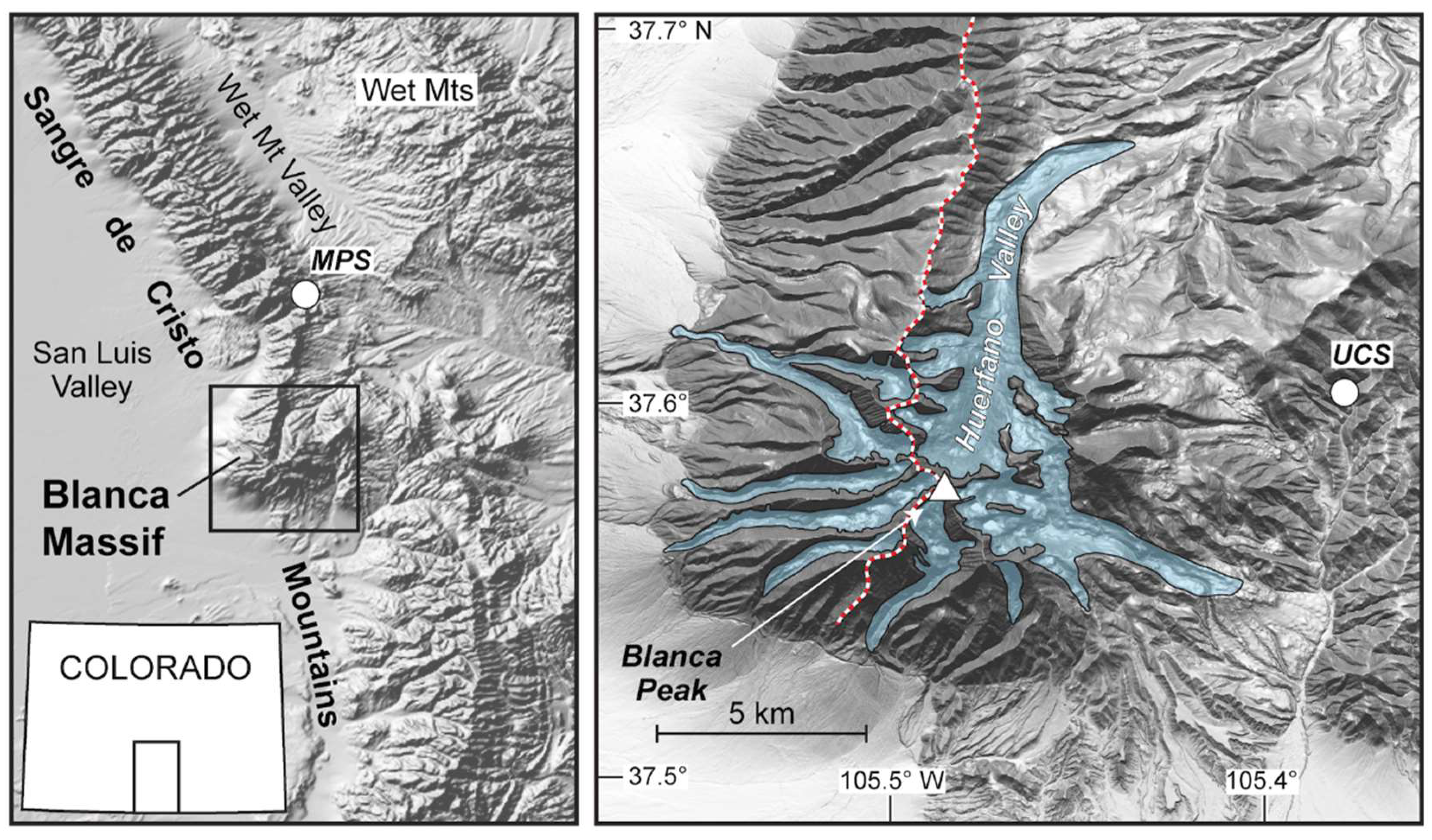
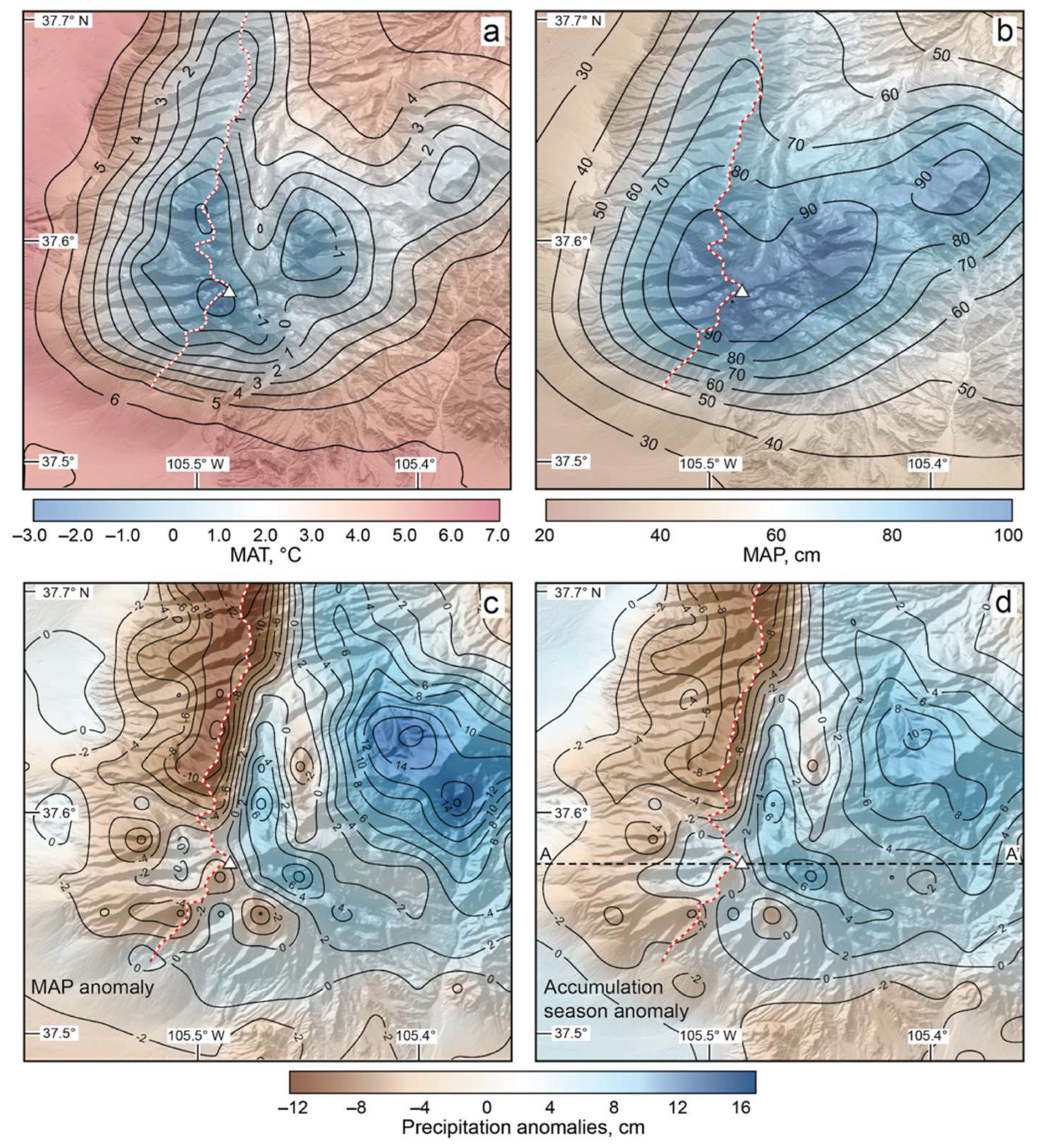
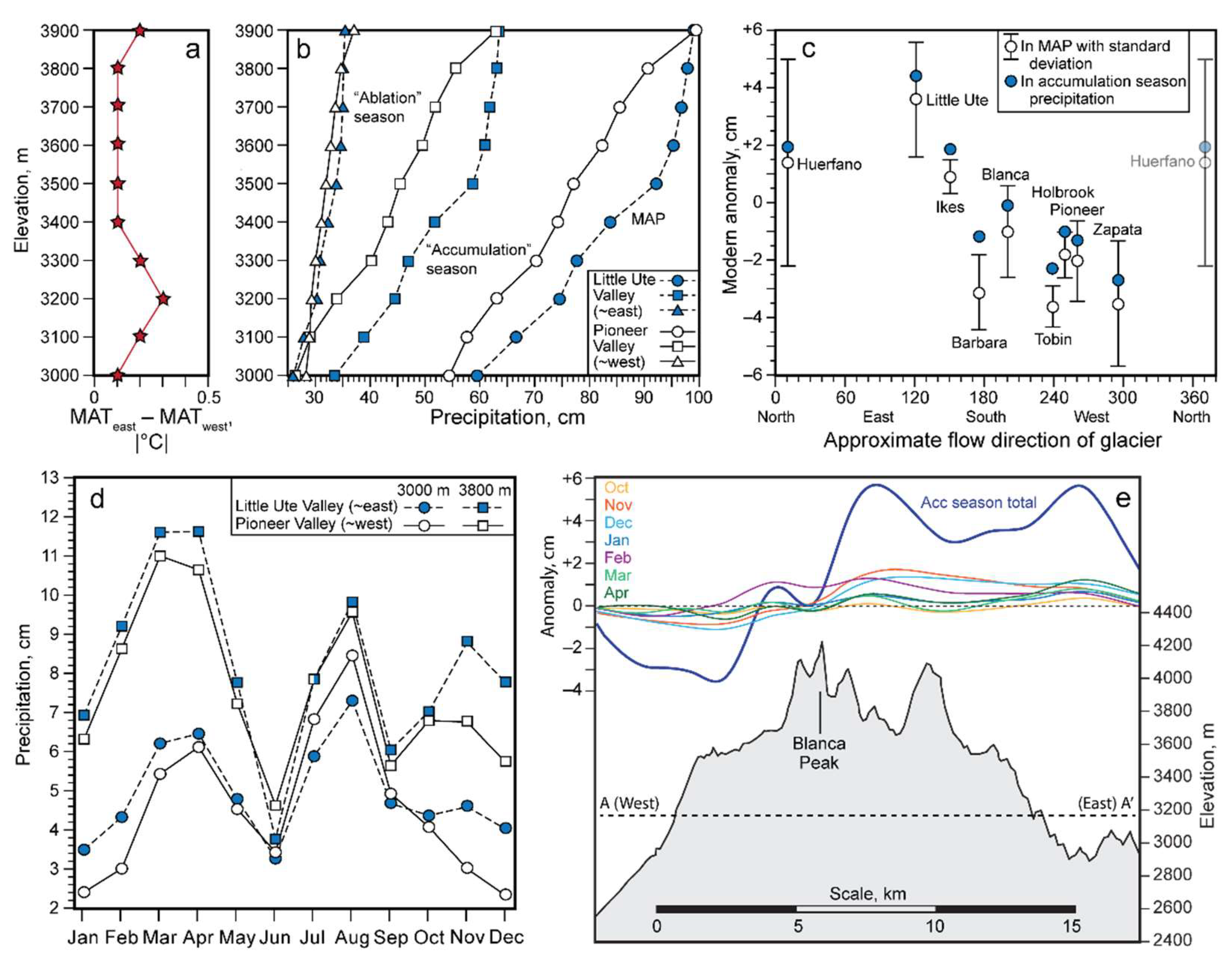
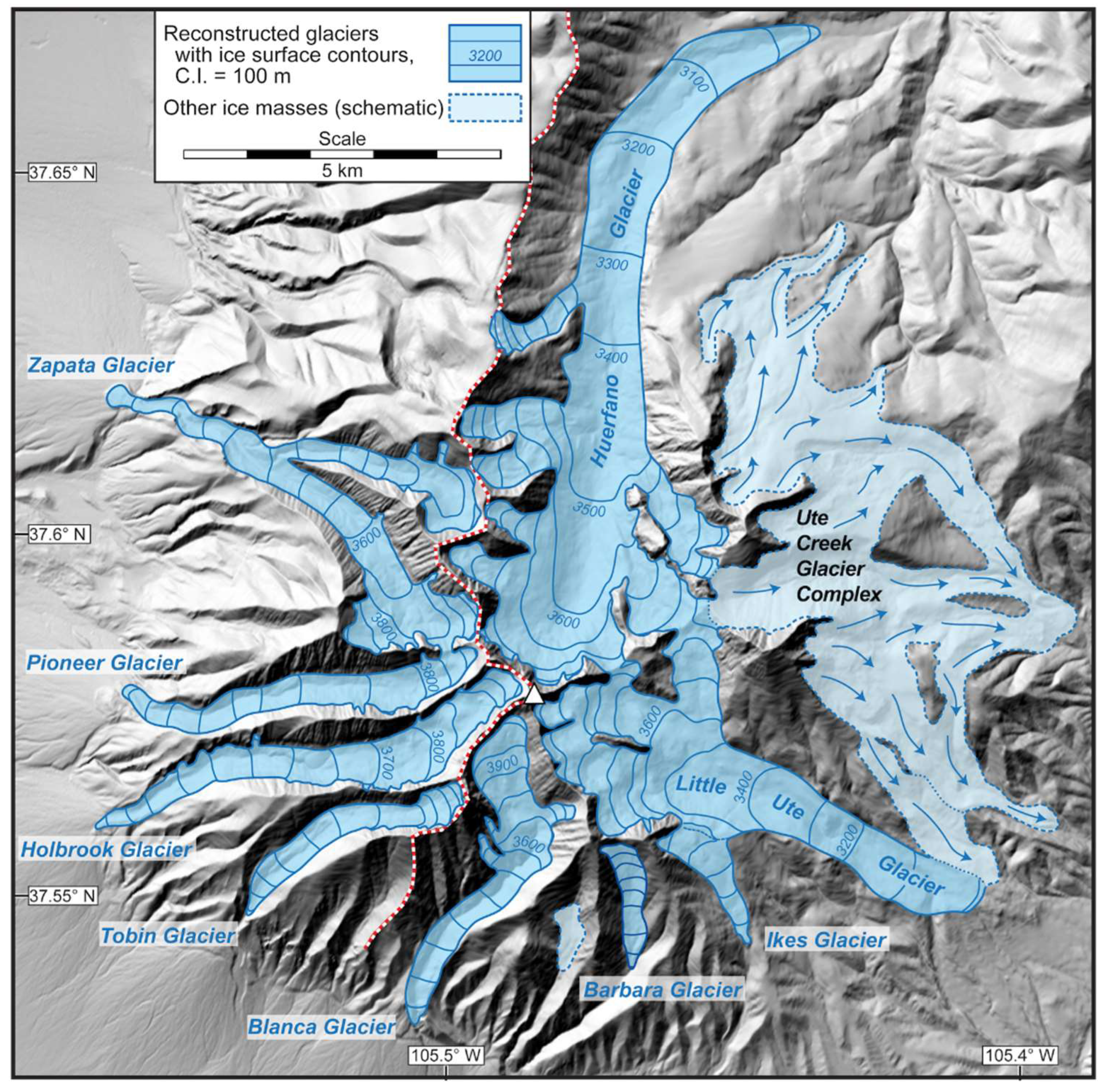
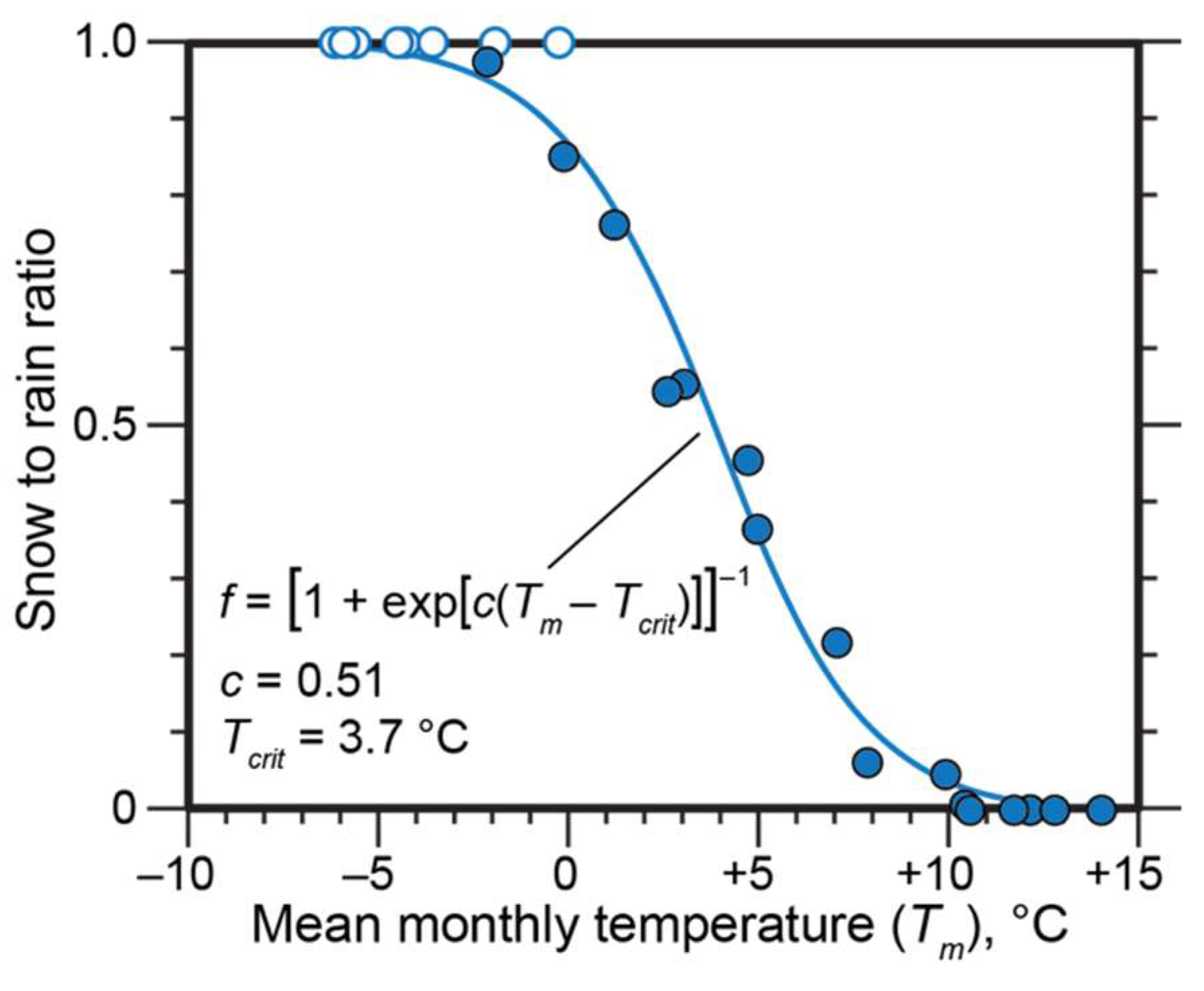
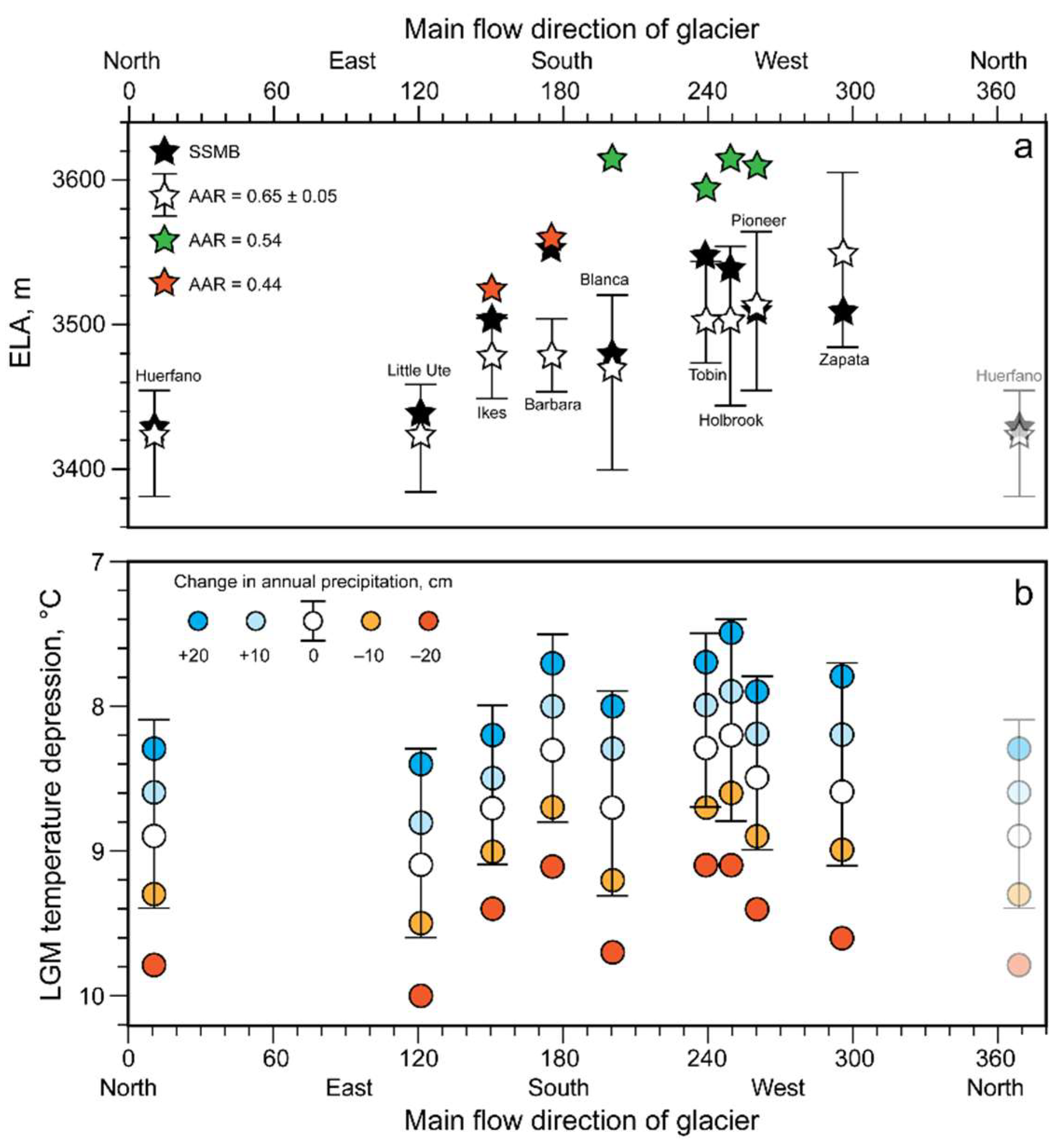
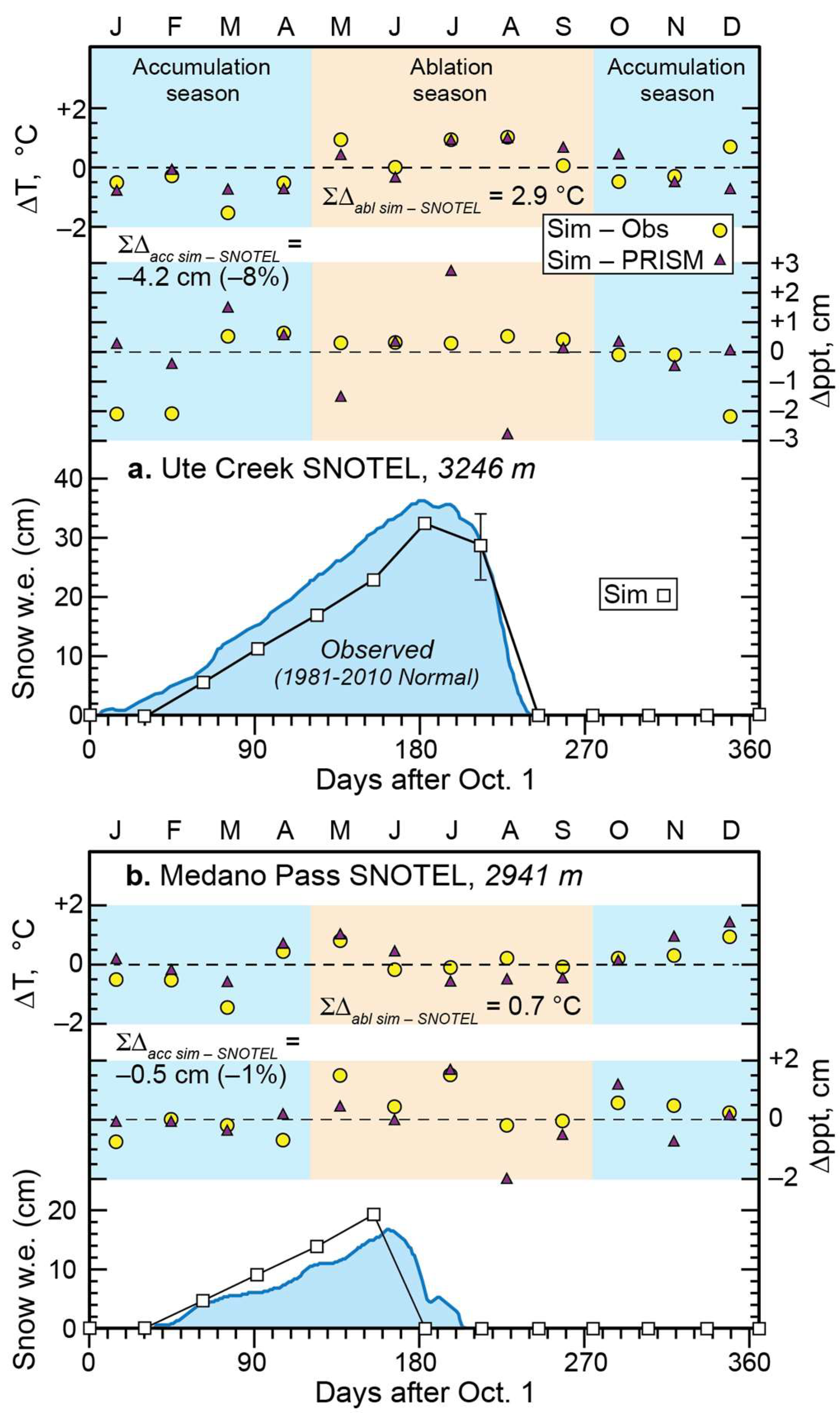
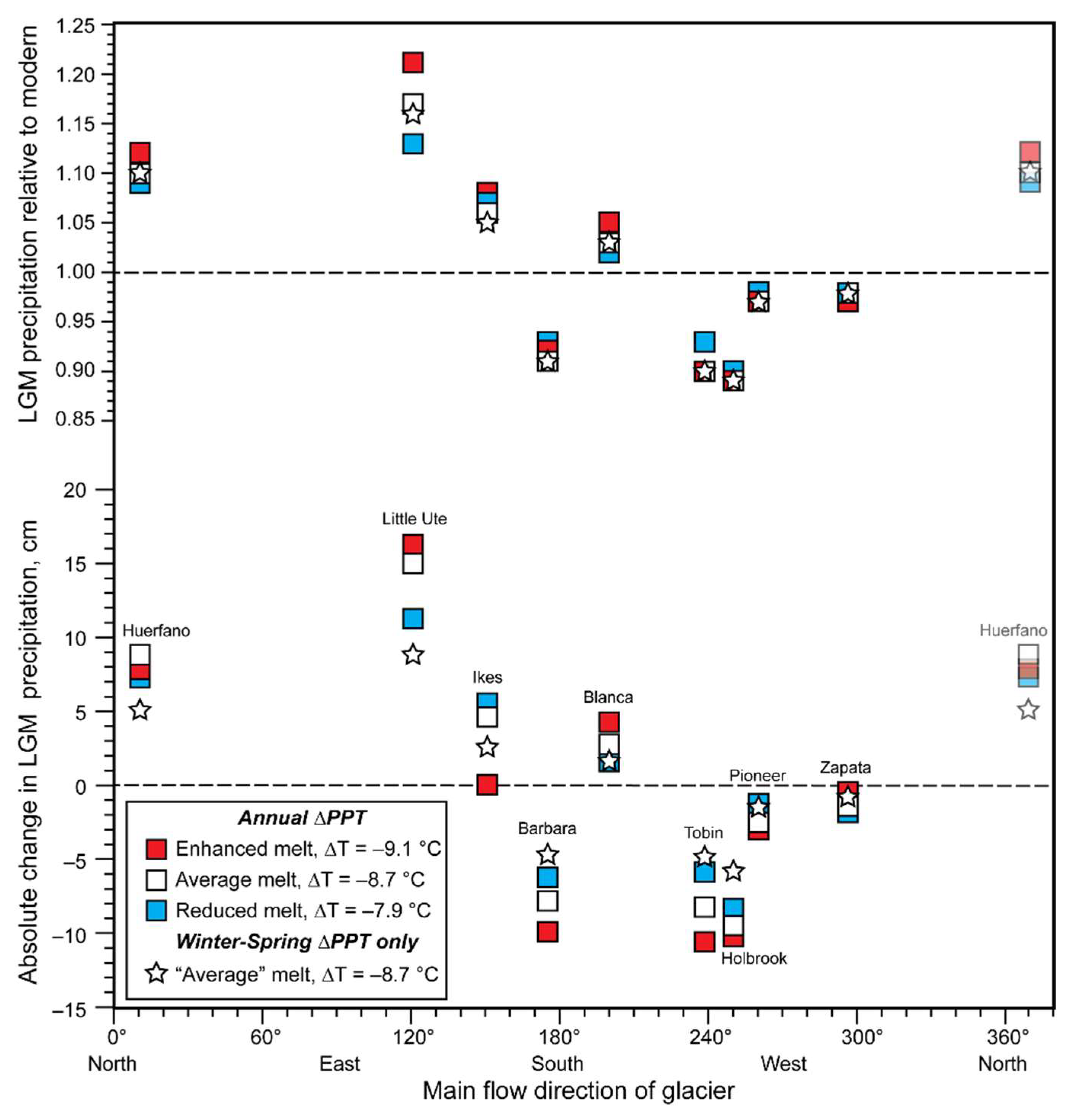
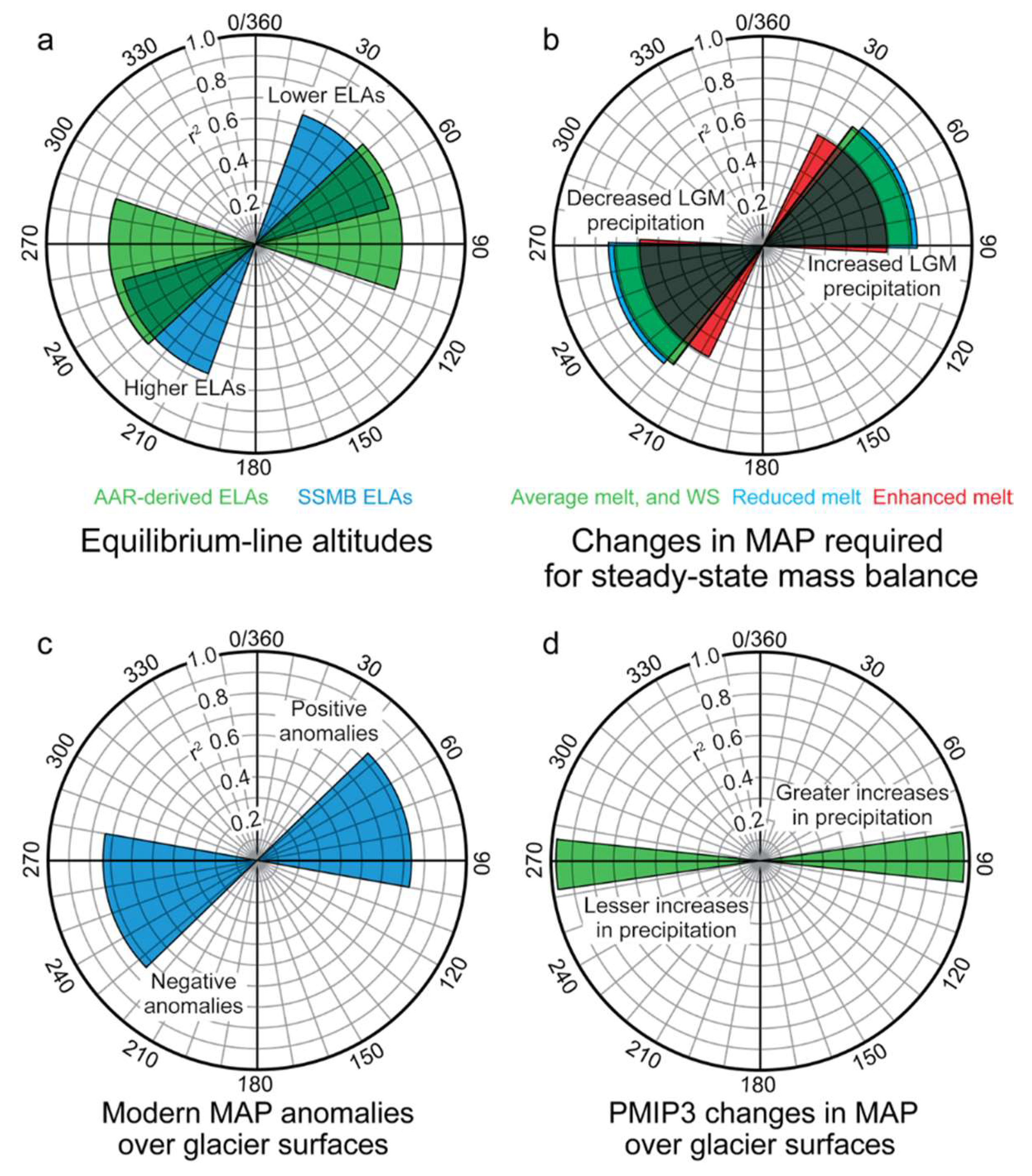
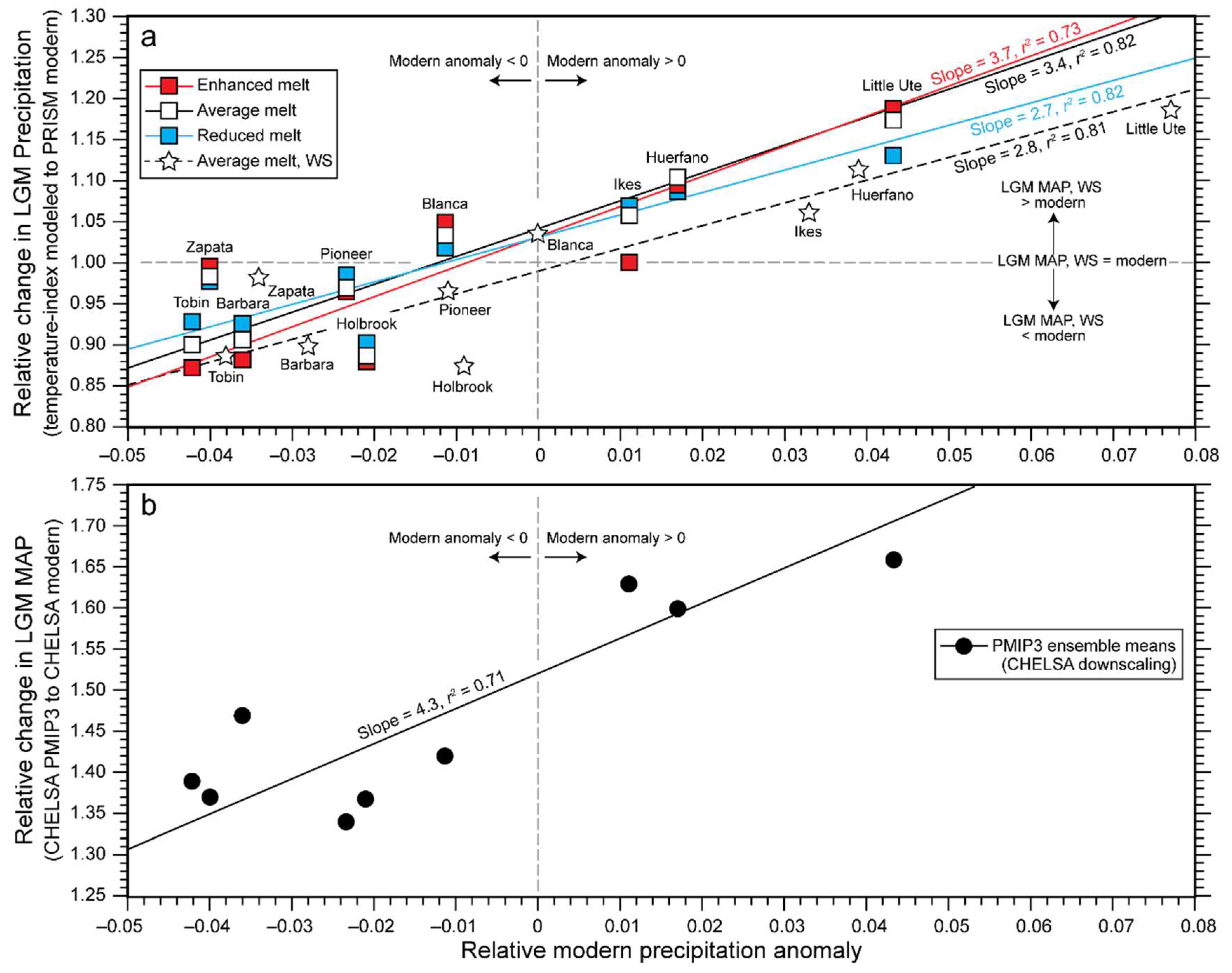
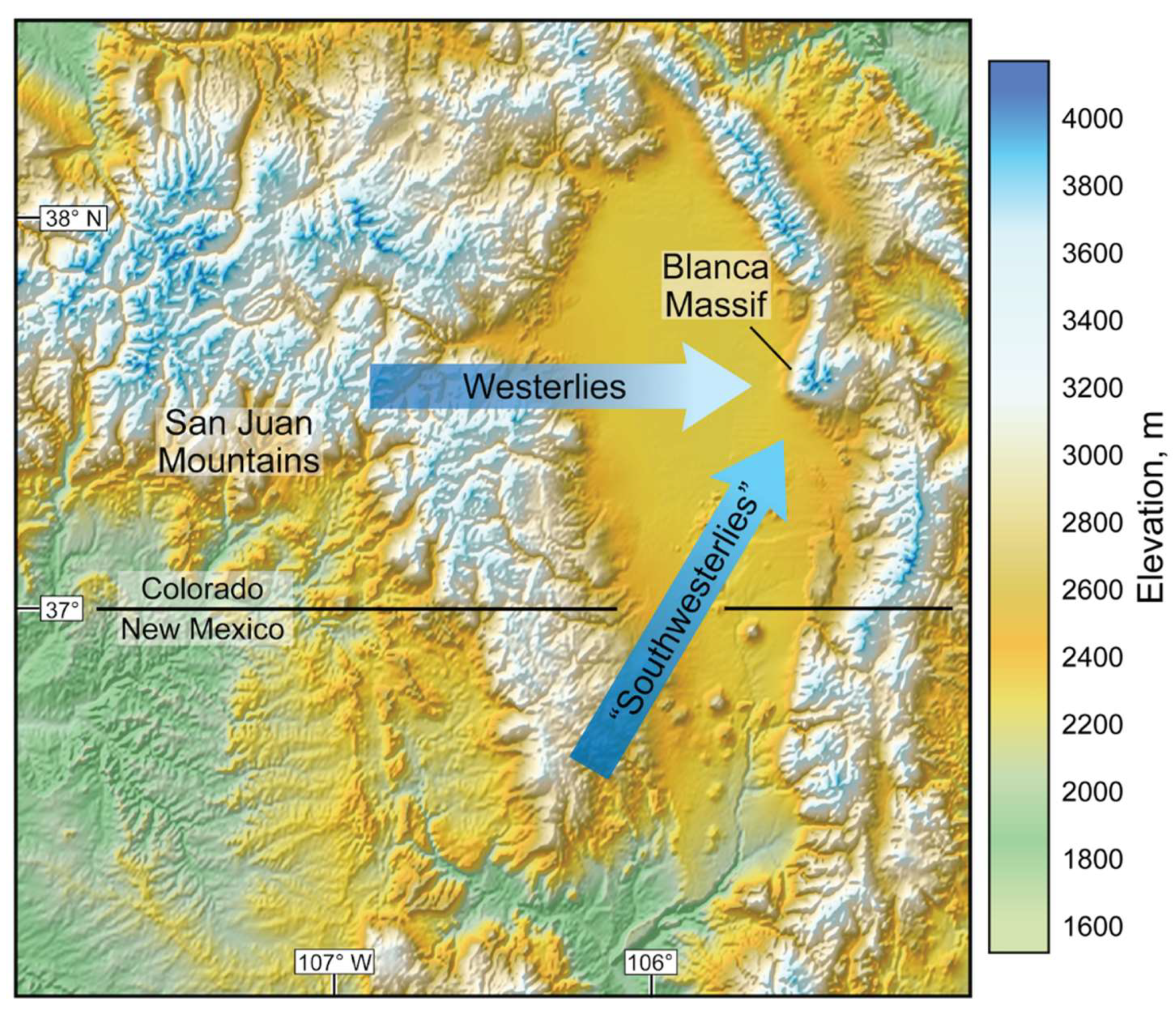
Table 1.
Surface area, length, mean, and maximum thickness, driving stresses, and AAR-derived ELAs of reconstructed glaciers.
Table 1.
Surface area, length, mean, and maximum thickness, driving stresses, and AAR-derived ELAs of reconstructed glaciers.
| Glacier | Area km2 | Length, km * | Average Ice Thickness, m *,† | Maximum Ice Thickness m *,† | Driving Stresses, kPa ** | AAR-Derived ELA, m † | ||
|---|---|---|---|---|---|---|---|---|
| AAR = 0.65 | AAR = 0.54 | AAR = 0.44 | ||||||
| Huerfano | 17.84 | 11.9 | 150 | 250 | 89–121 | 3425 | na | na |
| Little Ute | 9.32 | 8.1 | 70 | 130 | 72–138 | 3425 | na | na |
| Ikes | 0.84 | 2.7 | 25 | 55 | 52–88 | 3480 | na | 3525 |
| Barbara | 0.65 | 2.3 | 20 | 55 | 76–150 | 3480 | na | 3560 |
| Blanca | 3.06 | 6.2 | 60 | 130 | 99–148 | 3470 | 3615 | na |
| Tobin | 1.53 | 4.2 | 35 | 80 | 46–142 | 3505 | 3590 | na |
| Holbrook | 3.63 | 7.4 | 60 | 125 | 56–116 | 3505 | 3615 | na |
| Pioneer | 2.45 | 5.9 | 55 | 100 | 64–109 | 3515 | 3610 | na |
| Zapata | 5.46 | 7.4 | 55 | 100 | 51–101 | 3550 | na | na |
* Longest flow line where applicable; † nearest 5 m; ** calculated at a number of ice surface contours.
Table 2.
Derived temperature depression and ELAs based on steady-state mass balance of paleoglaciers. Temperatures are reported to nearest tenth of a degree. Changes in precipitation are those in mean annual.
Table 2.
Derived temperature depression and ELAs based on steady-state mass balance of paleoglaciers. Temperatures are reported to nearest tenth of a degree. Changes in precipitation are those in mean annual.
| Model Parameter | Temperature Depression, °C | Steady-State ELA, m * | ||||||
|---|---|---|---|---|---|---|---|---|
| Precipitation Change (F), cm | 0 | 10 | 20 | −10 | −20 | |||
| Melt Factors (mƒ) Snow/Ice | 0.0045/0.008 | 0.0065/0.010 | 0.0025/0.006 | 0.0045/0.008 | ||||
| m w.e. °C−1 d−1 | (Average Melt) | (Enhanced Melt) | (Reduced melt) | |||||
| Glacier | ||||||||
| Huerfano | 8.9 | 9.4 | 8.1 | 8.6 | 8.3 | 9.3 | 9.8 | 3430 |
| Little Ute | 9.1 | 9.6 | 8.3 | 8.8 | 8.4 | 9.5 | 10 | 3440 |
| Ikes | 8.7 | 9.1 | 8 | 8.5 | 8.2 | 9 | 9.4 | 3505 |
| Barbara | 8.3 | 8.8 | 7.5 | 8 | 7.7 | 8.7 | 9.1 | 3555 |
| Blanca | 8.7 | 9.3 | 7.9 | 8.3 | 8 | 9.2 | 9.7 | 3480 |
| Tobin | 8.3 | 8.7 | 7.5 | 8 | 7.7 | 8.7 | 9.1 | 3555 |
| Holbrook | 8.2 | 8.8 | 7.4 | 7.9 | 7.5 | 8.6 | 9.1 | 3540 |
| Pioneer | 8.5 | 9 | 7.8 | 8.2 | 7.9 | 8.9 | 9.4 | 3510 |
| Zapata | 8.6 | 9.1 | 7.7 | 8.2 | 7.8 | 9 | 9.6 | 3510 |
| Means | 8.6 ± 0.3 | 9.1 ± 0.3 | 7.8 ± 0.3 | 8.3 ± 0.3 | 7.9 ± 0.3 | 9.0 ± 0.3 | 9.5 ± 0.3 | |
* Nearest 5 m; for F = 0, mf = 0.0045/0.008 m w.e. °C−1 d−1.
Table 3.
Changes in mean annual (∆MAP) or winter/spring precipitation (∆WS) required for steady-state mass balance under the assumptions of uniform LGM temperature depression, ∆T. Percentages are rounded to nearest whole number.
Table 3.
Changes in mean annual (∆MAP) or winter/spring precipitation (∆WS) required for steady-state mass balance under the assumptions of uniform LGM temperature depression, ∆T. Percentages are rounded to nearest whole number.
| Glacier | Average Melt | Enhanced Melt | Reduced Melt | Average Melt | |
|---|---|---|---|---|---|
| ∆T, °C | 8.6 | 9.1 | 7.8 | 8.6 | |
| mf | 0.0045/0.008 | 0.0065/0.010 | 0.0025/0.006 | 0.0045/0.008 | |
| ∆MAP, cm (%) | ∆MAP, cm (%) | ∆MAP, cm (%) | ∆WS, cm (%) | ||
| Huerfano | 8.7 (10) | 7.9 (9) | 7.2 (9) | 5.1 (10) | |
| Little Ute | 15.0 (17) | 16.2 (19) | 11.3 (13) | 8.8 (16) | |
| Ikes | 4.6 (6) | 0.0 (0) | 5.6 (7) | 2.7 (5) | |
| Barbara | −7.8 (−9) | −9.9 (−12) | −6.2 (−7) | −4.6 (−9) | |
| Blanca | 2.9 (3) | 4.2 (5) | 1.6 (2) | 1.7 (3) | |
| Tobin | −8.2 (−10) | −10.5 (−13) | −5.9 (−7) | −4.8 (−10) | |
| Holbrook | −9.5 (−11) | −10.1 (−12) | −8.3 (−10) | −5.7 (−11) | |
| Pioneer | −2.5 (−3) | −3.0 (−4) | −1.3 (−2) | −1.5 (−3) | |
| Zapata | −1.4 (−2) | −0.4 (0) | −1.9 (−2) | −0.8 (−2) |
Table 4.
Circular linear correlations of ELAs, required changes in precipitation to maintain steady-state mass balance (SSMB) of paleoglaciers under different scenarios, modern precipitation anomalies, and changes in precipitation indicated by PMIP3 ensembles, and 95% confidence intervals about maximums obtained by a cosinor technique. Null hypothesis that data are normally distributed is accepted when p values for Shapiro–Wilk criteria (test statistic is W) exceed 0.05.
| Data Set | Shapiro–Wilk | Circular Correlation | Confidence Interval about Maximum | |||
|---|---|---|---|---|---|---|
| W | p | r2 | p | Lower Bound | Upper Bound | |
| (Compass Directions, °) | ||||||
| AAR-derived ELAs | 0.94 | 0.56 | 0.70 | <0.006 | 227 | 287 |
| SSMB-ELAs | 0.91 | 0.31 | 0.66 | <0.009 | 200 | 255 |
| ∆MAP, average melt | 0.94 | 0.58 | 0.71 | <0.005 | 37 | 90 |
| ∆MAP, enhanced melt | 0.92 | 0.41 | 0.59 | <0.017 | 26 | 93 |
| ∆MAP, reduced melt | 0.94 | 0.68 | 0.73 | <0.004 | 40 | 91 |
| ∆WS, average melt | 0.94 | 0.62 | 0.71 | <0.005 | 37 | 90 |
| Modern anomalies | 0.91 | 0.31 | 0.73 | <0.004 | 46 | 100 |
| ∆MAP, PMIP3 | 0.91 | 0.30 | 0.98 | <0.001 | 82 | 96 |
Table 5.
Mean LGM temperature depression over the study area and change in MAP (∆MAP) for individual glacier areas based on the CHELSA downscaling of PMIP3 models and modern climate (1979–2013). Note that the standard deviation reported for the ensemble means reflects the spread in the results from individual models, not that for the grid values in the ensemble means.
| Model | TemperatureDepression, °C | ∆MAP, cm | ||||||||
|---|---|---|---|---|---|---|---|---|---|---|
| Huerfano | Little Ute | Ikes | Barbara | Blanca | Tobin | Holbrook | Pioneer | Zapata | ||
| NCAR-CCSM4 | 8.6 ± 0.2 | 23.8 ± 2.0 | 26.9 ± 1.2 | 26.9 ± 0.7 | 24.6 ± 1.3 | 21.8 ± 3.2 | 19.4 ± 3.4 | 18.6 ± 4.5 | 17.1 ± 3.9 | 18.3 ± 5.4 |
| MRI-CGCM3 | 6.7 ± 0.4 | 37.1 ± 2.6 | 38.2 ± 3.3 | 37.7 ± 1.2 | 38.7 ± 1.5 | 37.3 ± 3.8 | 36.2 ± 3.4 | 35.5 ± 4.3 | 34.1 ± 3.7 | 35.1 ± 5.4 |
| CNRM-CM5 | 5.8 ± 0.4 | 26.5 ± 2.1 | 28.2 ± 1.6 | 27.7 ± 0.9 | 26.0 ± 1.3 | 23.7 ± 3.4 | 21.8 ± 3.3 | 21.2 ± 4.3 | 20.0 ± 3.8 | 21.6 ± 5.2 |
| FGOALS-g2 | 15.2 ± 0.4 | 17.1 ± 2.0 | 18.7 ± 1.4 | 17.9 ± 0.9 | 15.5 ± 1.2 | 13.9 ± 2.7 | 12.6 ± 2.4 | 11.8 ± 3.6 | 10.7 ± 3.1 | 11.9 ± 4.4 |
| IPSL-CM5A-LR | 13.6 ± 0.6 | 1.8 ± 2.0 | 3.6 ± 1.5 | 3.2 ± 0.8 | −1.2 ± 1.0 | −2.4 ± 1.4 | −3.3 ± 1.4 | −3.9 ± 2.0 | −4.7 ± 1.7 | −4.1 ± 2.8 |
| MIROC-ESM | 13.6 ± 0.3 | 13.9 ± 2.1 | 17.6 ± 2.4 | 17.5 ± 0.8 | 12.4 ± 2.1 | 9.6 ± 1.8 | 8.3 ± 1.8 | 7.5 ± 2.3 | 6.9 ± 2.2 | 7.8 ± 3.2 |
| MPI-ESM-P | 8.9 ± 0.3 | 16.9 ± 2.0 | 17.9 ± 1.3 | 17.3 ± 0.8 | 14.9 ± 1.3 | 13.0 ± 2.9 | 11.6 ± 2.7 | 11.2 ± 3.5 | 10.2 ± 3.0 | 11.6 ± 4.2 |
| Ensemble mean | 10.4 ± 3.7 | 19.5 ± 11.1 | 21.6 ± 10.9 | 21.2 ± 10.9 | 18.7 ± 12.6 | 16.7 ± 12.5 | 15.2 ± 12.3 | 14.6 ± 12.3 | 13.5 ± 12.1 | 14.6 ± 12.2 |
| MAP, cm | ||||||||||
| CHELSA Modern | 32.6 ± 4.0 | 32.6 ± 3.4 | 33.8 ± 1.0 | 40.0 ± 0.4 | 40.1 ± 1.5 | 39.4 ± 1.2 | 39.5 ± 1.9 | 39.3 ± 1.7 | 39.9 ± 1.7 | |
Publisher’s Note: MDPI stays neutral with regard to jurisdictional claims in published maps and institutional affiliations. |
© 2021 by the authors. Licensee MDPI, Basel, Switzerland. This article is an open access article distributed under the terms and conditions of the Creative Commons Attribution (CC BY) license (https://creativecommons.org/licenses/by/4.0/).
Share and Cite
MDPI and ACS Style
Brugger, K.A.; Leonard, E.M.; Refsnider, K.A.; Dolan, P. Climate on the Blanca Massif, Sangre de Cristo Mountains, Colorado, USA, during the Last Glacial Maximum. Quaternary 2021, 4, 27. https://0-doi-org.brum.beds.ac.uk/10.3390/quat4030027
AMA Style
Brugger KA, Leonard EM, Refsnider KA, Dolan P. Climate on the Blanca Massif, Sangre de Cristo Mountains, Colorado, USA, during the Last Glacial Maximum. Quaternary. 2021; 4(3):27. https://0-doi-org.brum.beds.ac.uk/10.3390/quat4030027
Chicago/Turabian StyleBrugger, Keith A., Eric M. Leonard, Kurt A. Refsnider, and Peter Dolan. 2021. "Climate on the Blanca Massif, Sangre de Cristo Mountains, Colorado, USA, during the Last Glacial Maximum" Quaternary 4, no. 3: 27. https://0-doi-org.brum.beds.ac.uk/10.3390/quat4030027