Comparative Analysis of Classification Algorithms Using CNN Transferable Features: A Case Study Using Burn Datasets from Black Africans


Centre for Visual Computing, Faculty of Engineering and Informatics, University of Bradford, Bradford BD7 1DP, UK
†
Current address: Department of Computer Science, Faculty of Science, Gombe State University, Gombe P.M.B. 127, Nigeria.
Appl. Syst. Innov. 2020, 3(4), 43; https://0-doi-org.brum.beds.ac.uk/10.3390/asi3040043
Submission received: 22 August 2020
/
Revised: 28 September 2020
/
Accepted: 12 October 2020
/
Published: 14 October 2020
(This article belongs to the Special Issue Advanced Machine Learning Techniques, Applications and Developments)
Abstract
:Burn is a devastating injury affecting over eleven million people worldwide and more than 265,000 affected individuals lost their lives every year. Low- and middle-income countries (LMICs) have surging cases of more than 90% of the total global incidences due to poor socioeconomic conditions, lack of preventive measures, reliance on subjective and inaccurate assessment techniques and lack of access to nearby hospitals. These factors necessitate the need for a better objective and cost-effective assessment technique that can be easily deployed in remote areas and hospitals where expertise and reliable burn evaluation is lacking. Therefore, this study proposes the use of Convolutional Neural Network (CNN) features along with different classification algorithms to discriminate between burnt and healthy skin using dataset from Black-African patients. A pretrained CNN model (VGG16) is used to extract abstract discriminatory image features and this approach was due to limited burn images which made it infeasible to train a CNN model from scratch. Subsequently, decision tree, support vector machines (SVM), naïve Bayes, logistic regression, and k-nearest neighbour (KNN) are used to classify whether a given image is burnt or healthy based on the VGG16 features. The performances of these classification algorithms were extensively analysed using the VGG16 features from different layers.
1. Introduction
Burns are a devastating injury subjecting more than 11 million people to psychological trauma [1]. These injuries cause an estimated mortality rate of over 265,000 globally per year [2,3]. Over 90% of burn incidences are in low- and middle-income countries (LMICs), about 11 times higher than the number of reported cases in high-income countries (HICs). Affected individuals in LMICs face a long-term risk of psychological and physical abnormality with possible pernicious consequences to their families, societies, and the nation at large. The socioeconomic status in developing countries has been a major factor for the high incidence and high mortality rate [2]. Moreover, this has also been attributed to illiteracy, lack of proper child supervision, crowded settlements, and unemployment.
The socioeconomic conditions complicate the situation due to a lack of access to hospitals or burn centres and lack of modern objective diagnostic tools. Traditionally, burns are diagnosed by burn surgeons or health specialists through inspection; however, inaccuracy and a lack of standard guidelines for histological interpretation result in subjective assessment and sampling errors as a result of burn heterogeneity [4,5,6]. The most widely used objective assessment method these days is laser Doppler imaging (LDI) as an alternative [7]. LDI is used to assess burn depth by measuring the perfusion rate of burnt tissue where a high perfusion score signifies a superficial burn while measurements with low perfusion scores signify deep burns. LDI has advantages over traditional methods due to its ability to asses burn wounds with no physical contact; as such. patients are not subjected to unnecessary pain [8,9]. However, the cost of diagnosis using LDI is very expensive, the device is cumbersome, and scanning time takes approximately 4 s for a perfusion image [10].
Recently, the use of CNN was recognised due to its powerful capability to automatically extract generic discriminatory features. This breakthrough technology has been applied to different application domains such as face recognition [11], brain tumour detection [12], and crop disease detection [13]. Moreover, studies in [8,14] used pretrained CNN models for feature extraction and support vector machines for the classification of features. Both studies used an immediate layer after the feature extraction layer (convolution layers) for the feature extraction. The study in [1] used an average pooling layer (pool5) for feature extraction and support vector machines for feature classification. Similarly, the study in [14] used three VGGNet models independently (VGG16, VGG19, and VGG-Face) for feature extraction, and, in all three scenarios, the first fully connected layer was used for feature extraction, while a support vector machine was used for feature classification. An important thing to consider and worth investigating is the most robust features in terms of accuracy and time complexity during training. This study used a pretrained VGG16 model where features from the first and second fully connected (FC) layers were used for classification by different classifiers.
2. Materials and Methodology
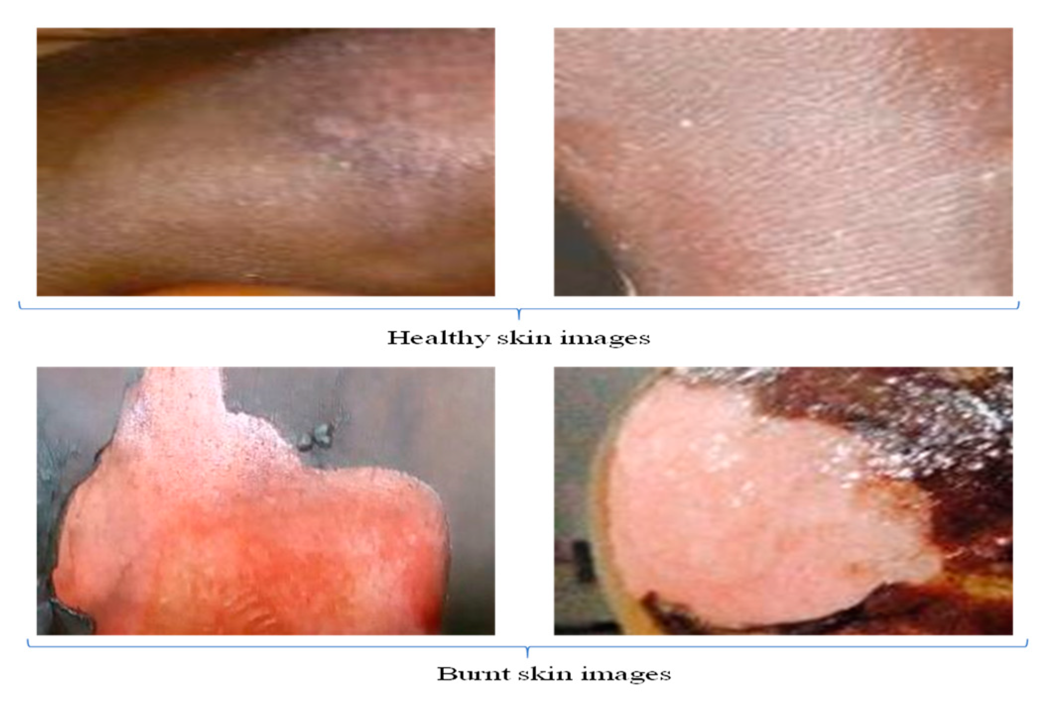
Burn images are crucial data needed to diagnose the wound and determine the precise treatment using machine learning algorithms. Although medical data are difficult to acquire due to confidentiality, the datasets were obtained from Federal Teaching Hospital Gombe in North-Eastern Nigeria, approved by the research and ethics committee. In total, 109 red/green/blue (RGB) images of patients were obtained, and all features that could result in patient identification such as faces were cropped out, as depicted in Figure 1. Then, different rectangular shapes of the burn’s representative areas were extracted from the images, resulting to 320 images per class. Furthermore, these images were subjected to transformation processes such as rotation, vertical flipping, and horizontal flipping, resulting in a considerably large dataset of 840 images per class.
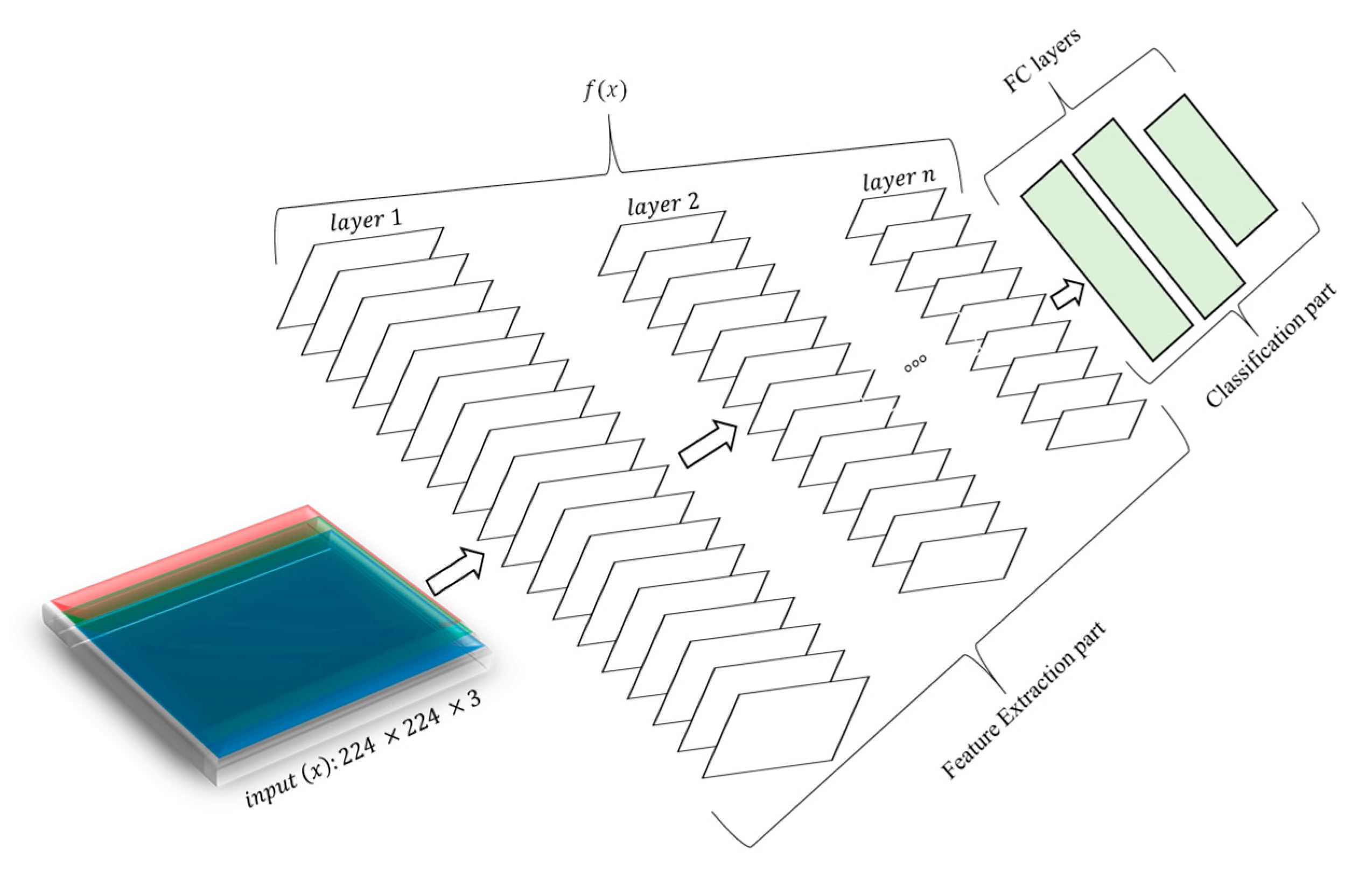
The methodology in this study consisted of two parts: feature extraction and feature classification. Figure 2 illustrates the methodology, starting from the input being processed in a feed-forward fashion and propagating from layer 1 to layer n. The convolutional layers along with other layers such as pooling, batch normalization, and activation layers denoted as served as feature extraction layers, while the dense layers (i.e., FC layers) served as classification layers. However, instead of retaining and retraining the FC layers, they were replaced with classification algorithm(s).
2.1. Extraction of Image Features
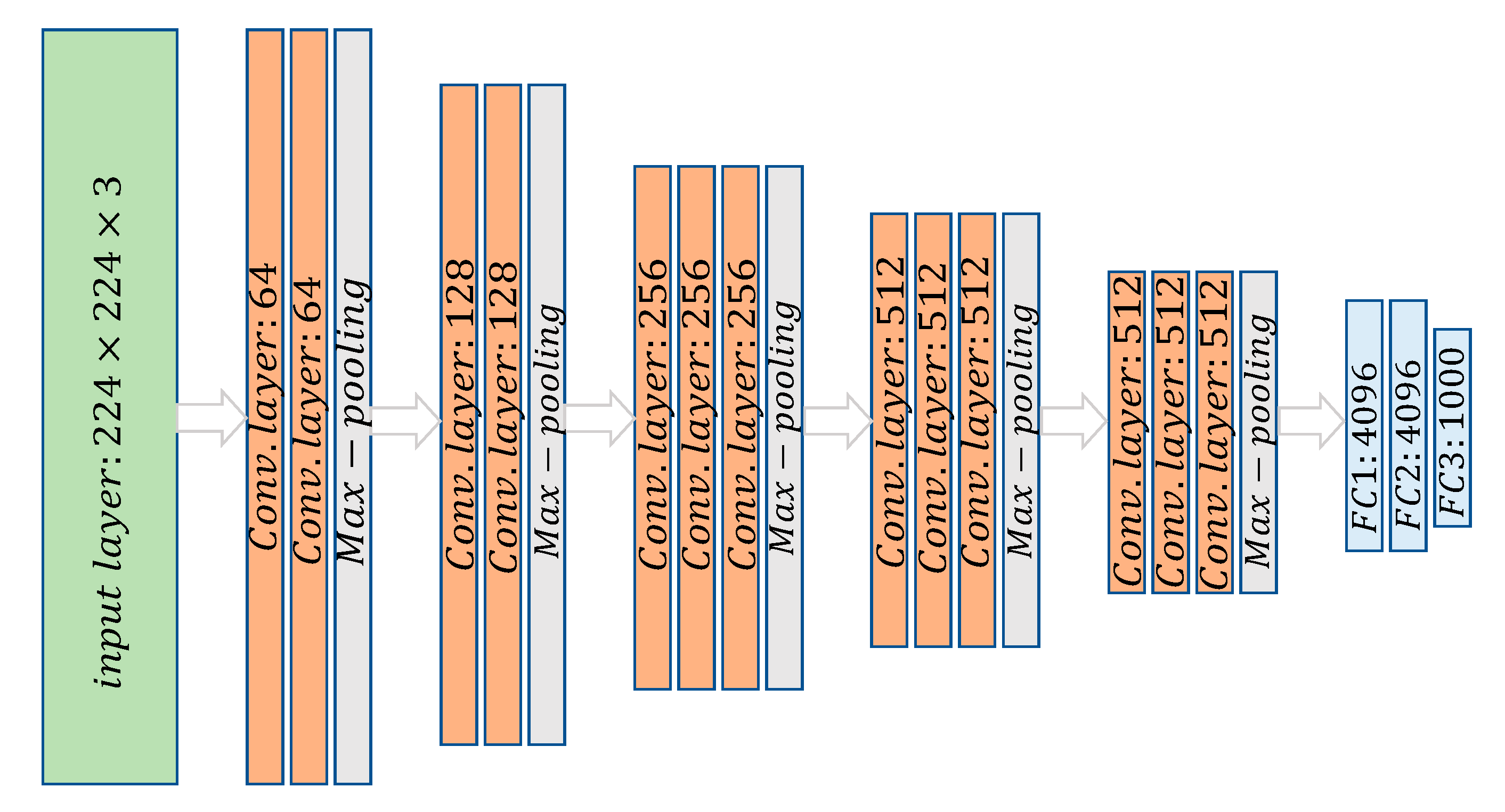
Here, VGG16 was used as a feature extractor because of its simplicity, and its architecture is illustrated in Figure 3. To extract features, the source model was entirely copied excluding the last classification layer and the copied layers were frozen. Freezing the layers ensures forward propagation while disabling backpropagation during training. Note that, for investigation purposes in this study, VGG16 was considered due to its architectural simplicity. VGG16 has five convolutional blocks, where the first block has two convolution layers with 64 filters each, the second block has two convolution layers with 128 filters, and the third block has three convolution layers with 256 filters, while the fourth and fifth blocks have three convolution layers each with 512 filters. All filters in the convolution layers have same size (i.e., size). The top layers are three FC layers where the first two (FC1 and FC2) have 4096 neurons, while FC3 has 1000 neurons. In order to enhance computational efficiency, VVG16 has a max-poling layer after each convolution.
Given an input denoted as , this can be represented as tensor , where is the height of the image, is the width of the image, and represents the colour channels. The layers of the pretrained VGG16 can be expressed as series of functions . Moreover, let us assume that are respective outputs from each layer in the model, then the intermediate -th layer’s output can be computed from function and learned weights through .
Note that each convolution layer learns different image features, whereby one layer may learn edges, another may learn horizontal lines or vertical lines, and the lower layers learn complex and generic features as the image propagates into deeper layers [15,16,17]. Therefore, in order to decide a specific layer to use for the extraction of features, we ensure the image passes through all feature extraction layers, which ensures that all relevant features learned by each layer were collected and ready for classification. As such, the decision now is between FC layers, although a study for facial recognition using deep learning features and support vector machines showed that the immediate FC layer after the last convolution layer yields strong discriminatory features [11]. Here, we tried to exploit discriminatory features from the first two FC layers of the VGG16 and compared different classification algorithms. Each classification algorithm was tried on both FC layers’ features.
2.2. Classification of Features
Feature extraction is one part of the problem-solving process, whereas the other part involves classification, which optimally discriminates the two given classes; it can be achieved using different available classification algorithms such as decision trees (DT), support vector machines (SVM), naïve Bayes, logistic regression, and k-nearest neighbour.
- DT is a classical classification supervised learning algorithm applied in different application domains such as medical diagnosis [18], signal processing [19], and intrusion detection [20]. It is a hierarchical classifier that builds a multi-label discrimination between classes to determine by determining their specific patterns, and it is very flexible in terms of handling both binary and multi-class classification problems [21].
- SVM is a supervised learning algorithm mostly used for binary classification [22]. It works by finding an optimal separating hyperplane (a decision boundary) that separate the two classes.
- Logistic regression (LR) is also used for binary classification problems [23]; it determines a relationship between categorical independent variables and dependent variables by evaluating probabilities using a logistic function. LR is computationally efficient and takes less time to train compared to SVM.
- The naïve Bayes (NB) classifier finds the probability of each class using a Bayesian formula [24,25]. It makes an assumption that all features of the samples in a particular class are independent of each other, and then discriminates the features by evaluating the posterior probability for each class, before allocating the feature to the class generating the maximum posterior probability.
- K-nearest neighbour (KNN) is a nonparametric classification algorithm that discriminates instances into their distinct classes according to the degree of likeness [24]. The input datasets are separated into K groups with during training where each instance is composed of features belonging to its group.
These classifiers were trained one at a time to predict burns and healthy skin as shown in Figure 4. Each classifier was separately trained using two sets of features (FC1 and FC2). The broken lines from FC2 into the individual classifiers indicate that these features were not passed into any of the classifiers once these classifiers were actively classifying FC1 features. The FC2 features were classified after the classifiers completed their task on the FC1 features. The accuracy and training time of each classifier was then computed.
2.3. Training Process
This section presents the training of the classifiers using the CNN transferable features. One way to train a chosen classifier is to divide the extracted features into two parts: one for training and the other for testing. The reason for this is that training and testing the classifier using same data cannot give a true estimate of the classifier’s performance. This approach, also known as the train–test split (TTS) is very efficient and less computationally expensive since it involves training only a single classifier in each run. However, the training or testing split may not contain strong representation patterns, which may lead to a biased system. Secondly, the TTS approach is prone to overfitting.
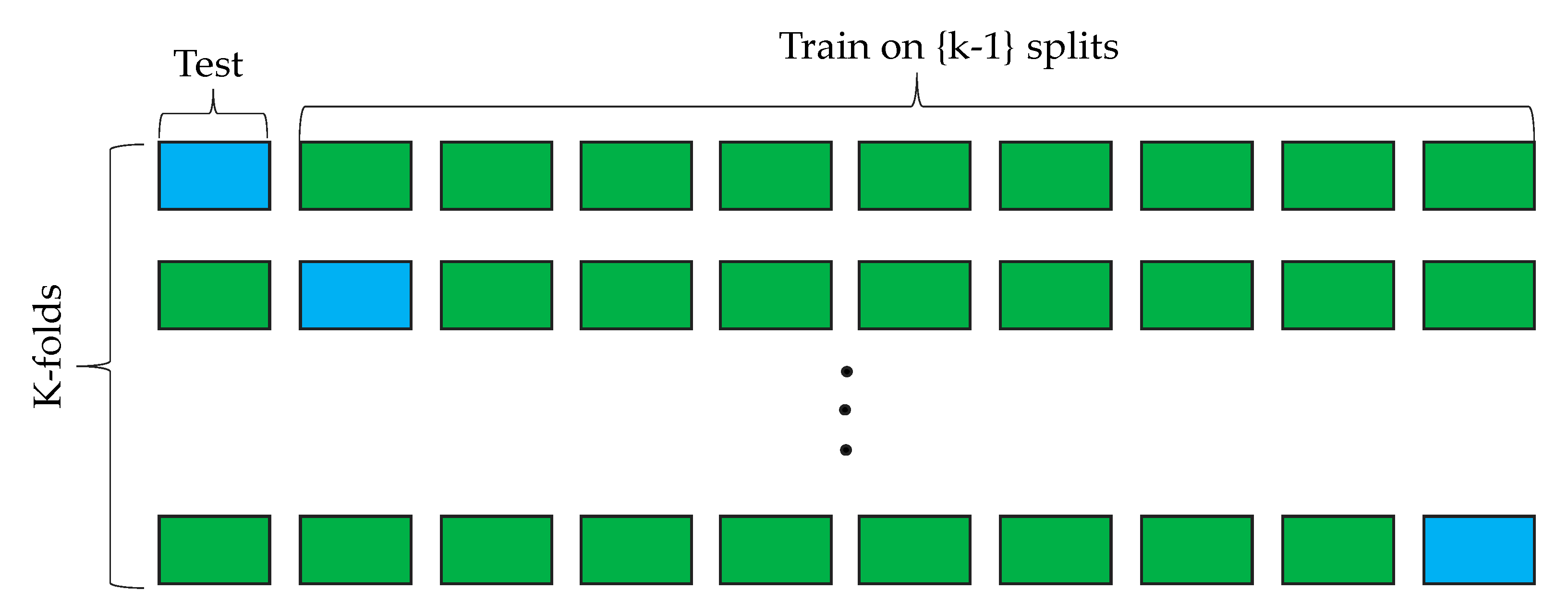
Alternatively, although it is more computationally expensive than TTS, cross-validation (CV) is an interesting technique which mitigates overfitting and captures the representation of each instance during both training and testing processes, thereby giving an optimum performance estimate of the classification algorithm. A common CV technique is -fold cross-validation, where k is the number of folds or parts into which the features are divided. The choice for k takes different values; most commonly, choices are k = 3, k = 5, and k = 10. When the value of k = 10, this means that 10% of the features are held out for testing, while the remaining 90% are used for training. This process is repeated k-times, whereby, at each run, a different fold is used for testing. Logically, training using k-fold CV ensures that k-classifiers are trained, and the mean score of their accuracies gives the overall performance estimate. Due to its significant impact on mitigating overfitting and its performance effectivity, all classifiers in this study were trained using the CV technique. Figure 5 depicts the CV technique used in this paper where k = 10.
3. Results and Discussion
In this section, experimental results are presented along with the explanation in detail. Table 1 shows the overall accuracy of each classifier from the features of FC1 and FC2 layers. Deep burn features from FC1 and FC2 layers for classification using the DT algorithm are presented in the Table 1. Both FC layers had 4096 feature vectors, but FC1 had 102,764,544 trainable parameters while FC2 had 16,781,312 trainable parameters. The DT classifier performed marginally better using deep FC2 features than FC1 features. Similarly, SVM and KNN achieved higher classification accuracy using FC2 features. It is also worth noting that the training of the classification algorithms had no random effect; hence, a random seed was used to ensure that the result was reproducible. By doing so, each algorithm was trained using the same splits and in exactly the same way. This implies that execution started at the same place every time for each classifier, which simply means that the experiment was fully deterministic.
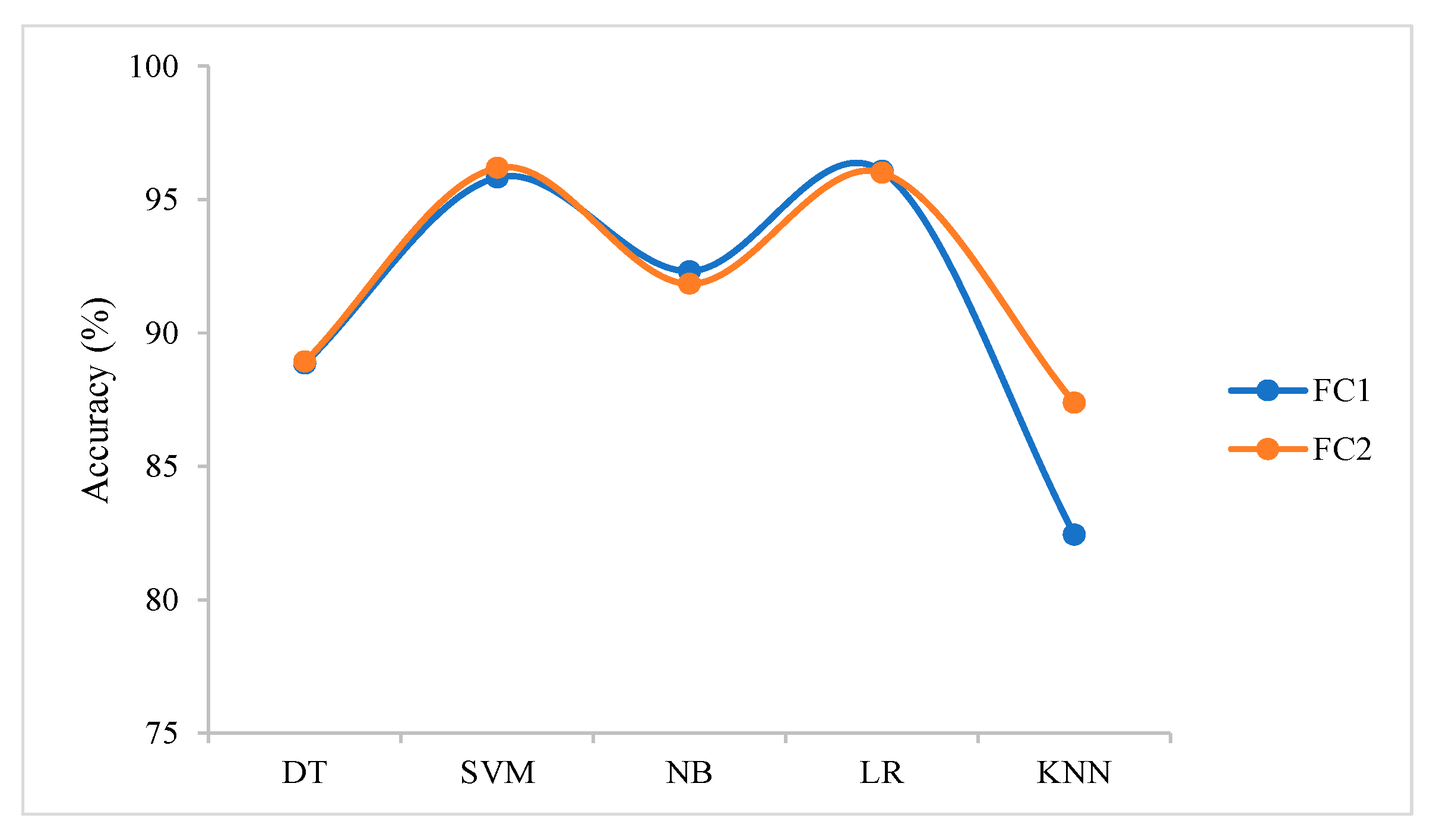
The result in Table 1 shows that DT performed slightly better with 4096 features of the FC2 layer, achieving 88.93% accuracy, than when using the same number of features from the FC1 layer (88.86%). SVM achieved 96.19% accuracy with FC2 features compared to 95.83% with FC1 features. Similarly, an accuracy of 87.38% was achieved using 4096 FC2 features by KNN compared to 82.44% using 4096 FC1 features. Two classification algorithms (NB and LR), in contrast, achieved higher accuracy using FC1 features than FC2 features. The NB classifier recorded an accuracy of 92.32% using FC1 features compared to 91.85% with FC2 features, whereas LR achieved an accuracy of 96.07% using FC1 features, which was marginally better than 96.01% with FC2 features.
Moreover, it is also obvious from Figure 6 that the best classification outputs came from the SVM classifier, followed by LR. The results suggest that, for FC2 features, SVM was most appropriate and effective, but LR was more suitable for use with FC1 features. This vitally shows that a good result can only be determined through trial and error rather than using theoretical and mathematic proofs.
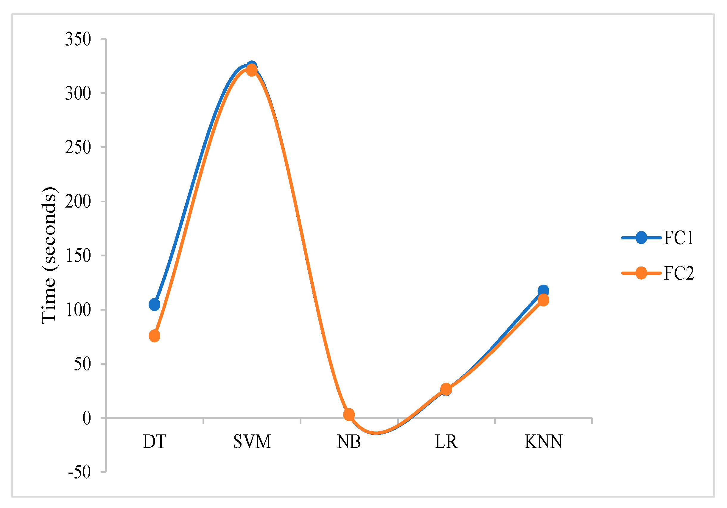
Furthermore, training time varied even though the same number of features was used from each FC layer, but Table 2 shows that all classifiers that returned the most impressive classification output using 4096 FC2 features took less time than when using FC1. DT was trained in 75.78 s with FC2 features compared to 104.75 s with FC1 features, SVM completed the training in 321.11 s with FC2 compared to 323.99 s with FC1 features, and KNN completed the training in 108.92 s with FC2 features compared to 117.09 s with FC1 features. Similarly, those classifiers that performed better with FC1 features also indicated more efficiency in terms of training time. NB completed the training in 2.91 s with FC1 features compared to 3.06 s with FC2 features, and LR completed the training in 26.10 s with FC1 features compared to 26.47 s with FC2 features.
Figure 7 presents a graphical visualisation of the training time complexity with NB as the most efficient classifier, taking a very short time to complete the training.
Performance Evaluation
Performance evaluation measures in classification problems are determined from a matrix (multidimensional table) showing examples of correctly and incorrectly classified instances from each class, known as a confusion matrix. The confusion matrix for a binary classification problem has two classes: positive and negative, as shown in Table 3.
TN, FP, FN, and TP respectively denote true negatives (examples of correctly predicted negative images), false positives (examples of images incorrectly predicted as positive), false negatives (examples of images incorrectly predicted as negative), and true positives (examples of positive images that are predicted correctly).
Table 4, Table 5, Table 6, Table 7 and Table 8 show confusion matrices obtained using DT, SVM, NB, LR, and KNN, respectively, with deep features from the FC1 layer.
Table 9, Table 10, Table 11, Table 12 and Table 13 shows classification results from the DT, SVM, NB, LR, and KNN classifiers, respectively, using deep FC2 features.
The most common used evaluation measure is accuracy; Equation (1) shows how accuracy is computed, and the result is shown in Table 1. Accuracy evaluates the classifier effectiveness by giving the percentage of precisely classified samples. Error rate is a complement of accuracy which provides the percentage of incorrectly classified samples, which can be evaluated using Equation (2).
Other performance evaluation measures include recall, precision, and F1-score. Recall, also known as sensitivity, measures the proportion of positive samples classified as positive out of the total number of positive samples, which can be computed using Equation (3). Precision gives the percentage of relevant samples predicted by the classifier out of the total predicted instances, which can be computed using Equation (4). In order to have balanced recall and precision values, a harmonic mean of these values is computed to return a single metric referred to as the F1-score, which can be computed using Equation (5).
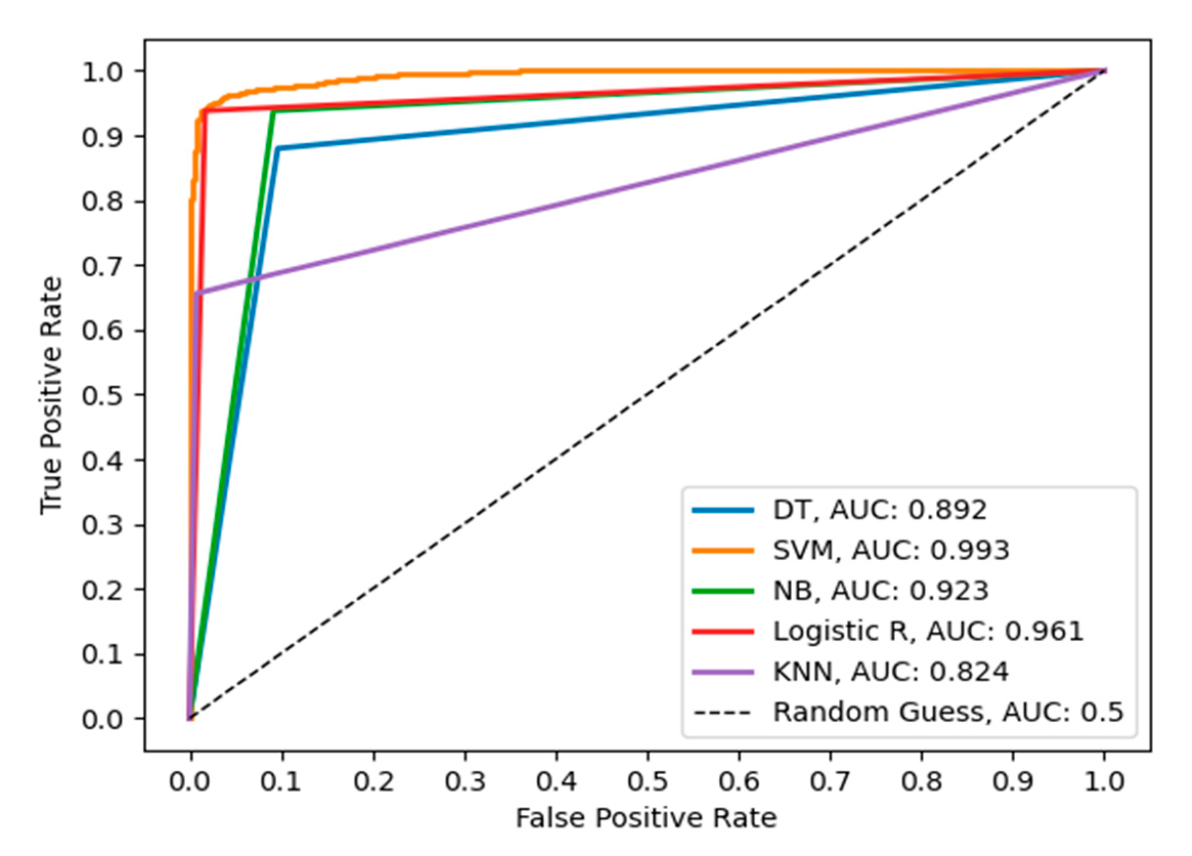
Moreover, other common performance evaluation measures for binary classification problems include the receiver operating characteristics (ROC) curve and precision–recall curve (PRC) [14,26]. The ROC curve is used to provide a graphical visualisation of the performance of a classification algorithm. The graph depicts the trade-off between the true positive rate (TPR) and the false positive rate (FPR). The area under the ROC curve (AUC) is widely used to evaluate the performance of the classifier. The values of the AUC range between 0 and 1, whereby an AUC value between 0 and 0.5 indicates poor classification while an AUC value ranging between 0.5 and 1.0 indicates good classification, and AUC = 1 indicates perfect classification. Figure 8 depicts the ROC curve of different classifiers using 4096 FC1 features of the VGG16 model. Here, the figure shows the true positive rate on the y-axis (vertical) and the true negative rate on the x-axis (horizontal). It is used to visualise how the classifier effectively separates the two classes. AUC provides the degree of separability by estimating how much the classifier is capable of discriminating the two classes, where a higher AUC denotes better classification of burns as burns and healthy skin as healthy skin. SVM produced a better discrimination output with AUC = 0.993, followed by LR with AUC = 0.961, NB with AUC = 0.923, DT with AUC = 0.892, and KNN with AUC = 0.824. A good classification model has AUC near to 1, which indicates good separability. A poor classification model has AUC near to 0, which indicates the worst measure of separability. On the other hand, an AUC of 0.5 tells us that a model has no capacity whatsoever in separating classes.
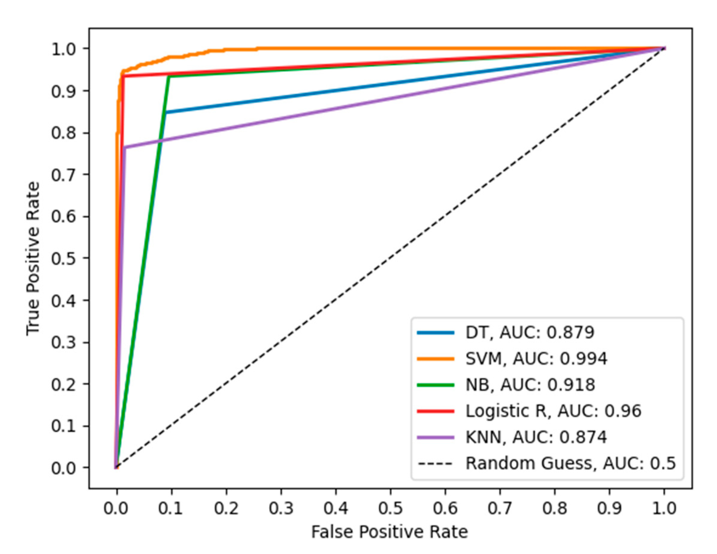
Figure 9 depicts the ROC curve of the different classifiers using 4096 FC2 features of the VGG16 model. Here, SVM also reported a better separability measure than the other classifiers.
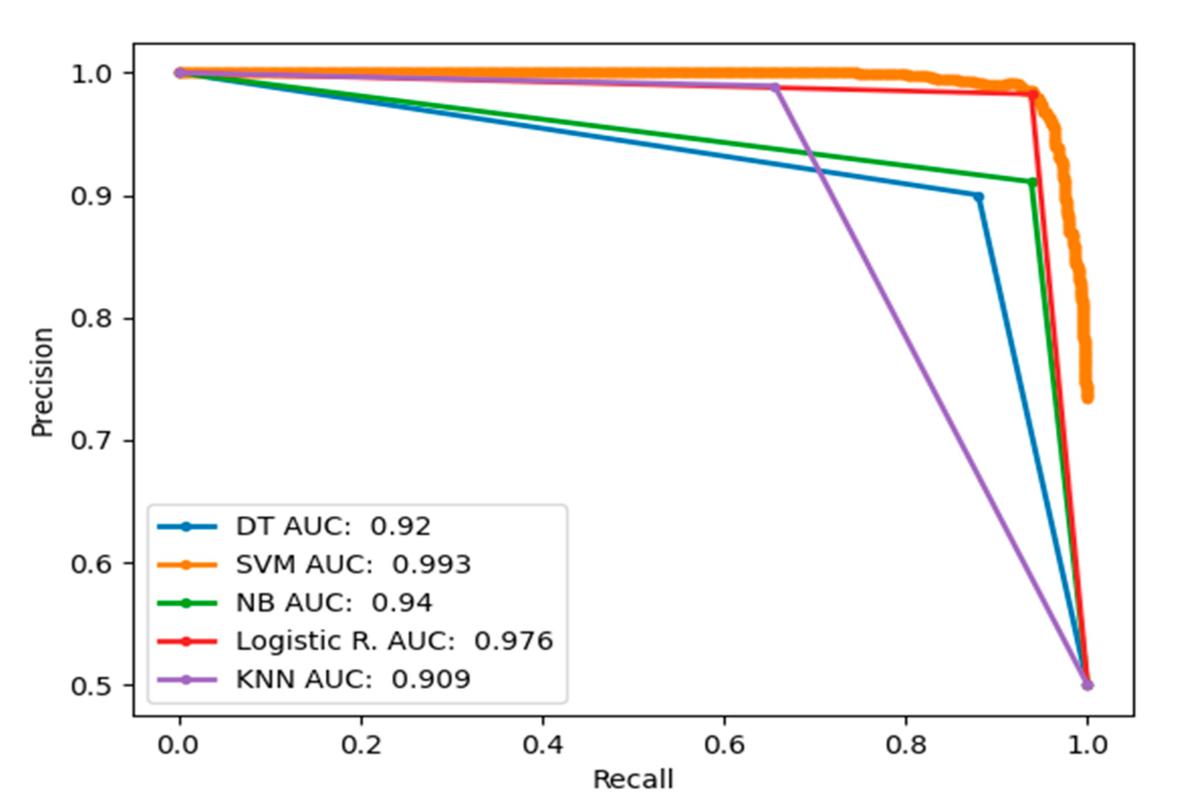
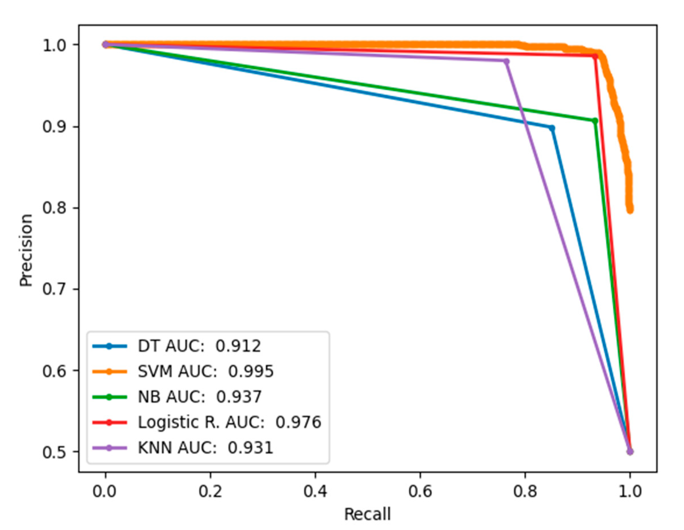
Furthermore, this study explored the use of the precision–recall curve (PRC) to provide graphical performance estimates using precision and recall performance evaluation measures. PRC has recall on the -axis and precision on the -axis. Recall gives the proportion of burn samples correctly classified out of the total burn samples, and precision gives the proportion of true positive samples out of the predicted burn samples. PRC has advantages over ROC because the latter tends to provide an overly convincing view of the performance of a classifier with class-imbalanced data. PRC is more informative than ROC and is appropriate for assessing the performance of less represented samples. PRC summarises a trade-off between true positive rate and positive predictive value. Figure 10 provides the PRC of different classifiers using 4096 FC1 features of the VGG16 model. Figure 11 provides the PRC of different classifiers using 4096 FC2 features of the VGG16 model. In both figures, AUC was used to summarise the performances of the classifiers, which a retuned an estimated value. A value near 1 indicates excellent classification accuracy and a value near 0 indicates poor classification outcome.
4. Conclusions
Training a CNN to classify a burn dataset is a difficult process because of the scarcity of images due several reasons such as privacy issues. For this reason, the concept of transfer learning, which involves reusing learnt weights of a CNN model trained on a different large dataset, can be used to solve another similar problem with deficient datasets. Transfer learning can used in two different ways: fine-tuning and feature extraction. The latter was used to extract off-the-shelf features, and DT, SVM, NB, LR, and KNN were trained independently to classify the features. Moreover, each classifier was trained using two different features extracted with the two different VGG16 layers.
In this study, it was found that some classifiers performed better when features were extracted from a specific CNN layer while others returned poor performances. These performances were analysed using different performance evaluation measures such as accuracy, time, ROC curve, AUC, and PRC. Comparatively, NB and LR achieved better classification results with FC1 features, while DT, SVM, and KNN achieved good classification results with FC2 features. This was reflected in Table 1 for accuracy and in Figure 6 and Figure 7.
Furthermore, this study discovered a great correlation between accuracy and training time for each classifier. DT was more efficient in terms of accuracy and training time when trained with FC2 features, where it achieved 88.93% accuracy in 75.78 s compared to 88.86% accuracy in 104.75 s using FC1 features. SVM achieved 96.19% accuracy in 321.11 s using FC2 features compared to 95.83% accuracy in 323.99 s using FC1 features. KNN achieved 87.38% accuracy in 108.92 s using FC2 features compared to 82.44% accuracy in 117.09 s using FC1 features. On the other hand, the NB classifier recorded 92.32% accuracy in 2.91 s using FC1 features compared to 91.85% accuracy in 3.06 s using FC2 features, and LR achieved a classification accuracy of 96.07% in 26.10 s using FC1 features compared to 96.01% accuracy in 26.47 s using FC2 features. This study can be extended further with different pretrained CNN models, as well as using a multi-class classification problem, particularly for different degrees of burns.
Funding
This research received no external funding.
Conflicts of Interest
The authors declare no conflict of interest.
References
- Grosu-Bularda, A.; Andrei, M.-C.; Mladin, A.D.; Ionescu, S.M.; Dringa, M.-M.; Lunca, D.C.; Lascar, I.; Teodoreanu, R.N. Periorbital lesions in severely burned patients. Rom. J. Ophthalmol. 2019, 63, 38–55. [Google Scholar] [CrossRef]
- Peck, M.D.; Toppi, J.T. Epidemiology and Prevention of Burns throughout the World. In Handbook of Burns; Springer: Berlin/Heidelberg, Germany, 2020; Volume 1, pp. 17–57. [Google Scholar]
- He, S.; Alonge, O.; Agrawal, P.; Sharmin, S.; Islam, I.; Mashreky, S.R.; El Arifeen, S. Epidemiology of Burns in Rural Bangladesh: An Update. Int. J. Environ. Res. Public Heal. 2017, 14, 381. [Google Scholar] [CrossRef] [PubMed]
- Abubakar, A.; Ugail, H.; Bukar, A.M.; Aminu, A.A.; Musa, A. Transfer Learning Based Histopathologic Image Classification for Burns Recognition. In Proceedings of the 2019 15th International Conference on Electronics, Computer and Computation (ICECCO), Abuja, Nigeria, 10–12 December 2019; Aminu, A.A., Musa, A., Eds.; Institute of Electrical and Electronics Engineers (IEEE): New York, NY, USA, 2019; pp. 1–6. [Google Scholar]
- Abubakar, A.; Ajuji, M.; Yahya, I.U. Comparison of Deep Transfer Learning Techniques in Human Skin Burns Discrimination. Appl. Syst. Innov. 2020, 3, 20. [Google Scholar] [CrossRef] [Green Version]
- Jaspers, M.; Van Haasterecht, L.; Van Zuijlen, P.P.; Mokkink, L.B. A systematic review on the quality of measurement techniques for the assessment of burn wound depth or healing potential. Burns 2019, 45, 261–281. [Google Scholar] [CrossRef] [PubMed]
- Mirdell, R.; Farnebo, S.; Sjöberg, F.; Tesselaar, E. Using blood flow pulsatility to improve the accuracy of laser speckle contrast imaging in the assessment of burns. Burns 2020, 46, 1398–1406. [Google Scholar] [CrossRef] [PubMed]
- Abubakar, A.; Ugail, H. Discrimination of Human Skin Burns Using Machine Learning; Springer: Cham, Switzerland, 2019; pp. 641–647. [Google Scholar]
- Abubakar, A.; Ugail, H.; Bukar, A.M. Assessment of Human Skin Burns: A Deep Transfer Learning Approach. J. Med. Biol. Eng. 2020, 40, 321–333. [Google Scholar] [CrossRef]
- Hoeksema, H.; Baker, R.; A Holland, A.J.; Perry, T.; Jeffery, S.; Verbelen, J.; Monstrey, S. A new, fast LDI for assessment of burns: A multi-centre clinical evaluation. Burns 2014, 40, 1274–1282. [Google Scholar] [CrossRef] [PubMed]
- Elmahmudi, A.; Ugail, H. Experiments on Deep Face Recognition Using Partial Faces. In Proceedings of the 2018 International Conference on Cyberworlds (CW), Singapore, 3–5 October 2018; Institute of Electrical and Electronics Engineers (IEEE): New York, NY, USA, 2019; pp. 357–362. [Google Scholar]
- Deepak, S.; Ameer, P. Brain tumor classification using deep CNN features via transfer learning. Comput. Biol. Med. 2019, 111, 103345. [Google Scholar] [CrossRef] [PubMed]
- Karthik, R.; Hariharan, M.; Anand, S.; Mathikshara, P.; Johnson, A.; Menaka, R. Attention embedded residual CNN for disease detection in tomato leaves. Appl. Soft Comput. 2020, 86, 105933. [Google Scholar]
- Abubakar, A.; Ugail, H.; Bukar, A.M. Noninvasive assessment and classification of human skin burns using images of Caucasian and African patients. J. Electron. Imaging 2019, 29, 041002. [Google Scholar] [CrossRef]
- Jilani, S.K.; Ugail, H.; Bukar, A.M.; Logan, A. On the Ethnic Classification of Pakistani Face using Deep Learning. In Proceedings of the 2019 International Conference on Cyberworlds (CW), Kyoto, Japan, 2–4 October 2019; pp. 191–198. [Google Scholar]
- Bukar, A.M. Automatic Age Progression and Estimation from Faces. Ph.D. Thesis, University of Bradford, Bradford, UK, 2019. [Google Scholar]
- Bukar, A.M.; Ugail, H. Automatic age estimation from facial profile view. IET Comput. Vis. 2017, 11, 650–655. [Google Scholar] [CrossRef] [Green Version]
- Mohsen, A.A.; Alsurori, M.; AlDobai, B.; Mohsen, G.A. New Approach to Medical Diagnosis Using Artificial Neural Network and Decision Tree Algorithm: Application to Dental Diseases. Int. J. Inf. Eng. Electron. Bus. 2019, 11, 52–60. [Google Scholar] [CrossRef]
- Jahmunah, V.; Oh, S.L.; Rajinikanth, V.; Ciaccio, E.J.; Cheong, K.H.; Arunkumar, N.; Acharya, U.R. Automated detection of schizophrenia using nonlinear signal processing methods. Artif. Intell. Med. 2019, 100, 101698. [Google Scholar] [CrossRef] [PubMed]
- Ahmim, A.; Maglaras, L.; Ferrag, M.A.; Derdour, M.; Janicke, H. A Novel Hierarchical Intrusion Detection System Based on Decision Tree and Rules-Based Models. In Proceedings of the 2019 15th International Conference on Distributed Computing in Sensor Systems (DCOSS), Santorini Island, Greece, 29–31 May 2019; Institute of Electrical and Electronics Engineers (IEEE): New York, NY, USA, 2019; pp. 228–233. [Google Scholar]
- Wang, F.; Wang, Q.; Nie, F.; Li, Z.; Yu, W.; Ren, F. A linear multivariate binary decision tree classifier based on K-means splitting. Pattern Recognit. 2020, 107, 107521. [Google Scholar] [CrossRef]
- Qian, Y.; Zhou, W.; Yan, J.; Li, W.; Han, L. Comparing machine learning classifiers for object-based land cover classification using very high resolution imagery. Remote. Sens. 2015, 7, 153–168. [Google Scholar] [CrossRef]
- Khairunnahar, L.; Hasib, M.A.; Bin Rezanur, R.H.; Islam, M.R.; Hosain, K. Classification of malignant and benign tissue with logistic regression. Inform. Med. Unlocked 2019, 16, 100189. [Google Scholar] [CrossRef]
- Farhi, L.; Zia, R.; Ali, Z.A. 5 Performance Analysis of Machine Learning Classifiers for Brain Tumor MR Images. Sir Syed Res. J. Eng. Technol. 2018, 1, 6. [Google Scholar] [CrossRef]
- Al Zorgani, M.; Ugail, H. Comparative Study of Image Classification Using Machine Learning Algorithms. Technical Report. 2018. Available online: https://www.semanticscholar.org/paper/EasyChair-Preprint-No-332-Comparative-Study-of-Zorgani-Ugail/6abe570933f798215534fb0ff168f42c118e5401?p2df (accessed on 14 October 2020).
- Fawcett, T. An introduction to ROC analysis. Pattern Recognit. Lett. 2006, 27, 861–874. [Google Scholar] [CrossRef]
Publisher’s Note: MDPI stays neutral with regard to jurisdictional claims in published maps and institutional affiliations. |
Figure 1.
Sample of the dataset.

Figure 2.
Methodology process.

Figure 3.
Architectural illustration of VGG16 model.

Figure 4.
Classification processes.

Figure 5.
Illustration of k-fold cross-validation (CV) technique.

Figure 6.
Comparison of transferable features and classifier performance.

Figure 7.
Training complexity of the classifiers.

Figure 8.
Receiver operating characteristics (ROC) curve comparing performances of the classifiers using 4096 FC1 features of the VGG16 model.
Figure 8.
Receiver operating characteristics (ROC) curve comparing performances of the classifiers using 4096 FC1 features of the VGG16 model.

Figure 9.
ROC comparing performances of the classifiers using 4096 FC2 features of the VGG16 model.

Figure 10.
Precision–recall curve (PRC) comparing performances of the classifiers using 4096 FC1 features of the VGG16 model.
Figure 10.
Precision–recall curve (PRC) comparing performances of the classifiers using 4096 FC1 features of the VGG16 model.

Figure 11.
PRC comparing performances of the classifiers using 4096 FC2 features of the VGG16 model.
Figure 11.
PRC comparing performances of the classifiers using 4096 FC2 features of the VGG16 model.


Table 1.
Classification accuracy. DT, decision tree; SVM, support vector machine; NB, naïve Bayes; LR, logistic regression; KNN, k-nearest neighbour; FC, fully connected.
Table 1.
Classification accuracy. DT, decision tree; SVM, support vector machine; NB, naïve Bayes; LR, logistic regression; KNN, k-nearest neighbour; FC, fully connected.
| Layer | DT | SVM | NB | LR | KNN |
|---|---|---|---|---|---|
| FC1 | 88.86% | 95.83% | 92.32% | 96.07% | 82.44% |
| FC2 | 88.93% | 96.19% | 91.85% | 96.01% | 87.38% |
Table 2.
Training time.
| Layer | DT | SVM | NB | LR | KNN |
|---|---|---|---|---|---|
| FC1 | 104.75 | 323.99 | 2.91 | 26.10 | 117.09 |
| FC2 | 75.78 | 321.11 | 3.06 | 26.47 | 108.92 |
Table 3.
Confusion matrix. TN, true negative; FN, false negative; TP, true positive; FP, false positive.
Table 3.
Confusion matrix. TN, true negative; FN, false negative; TP, true positive; FP, false positive.
| True Class | Predicted Class | |
|---|---|---|
| Negative | Positive | |
| Negative | TN | FP |
| Positive | FN | TP |
Table 4.
Deep FC1 features and DT classifier.
| True Class | Predicted Class | |
|---|---|---|
| Negative | Positive | |
| Negative | 761 | 79 |
| Positive | 97 | 743 |
Table 5.
Deep FC1 features and SVM classifier.
| True Class | Predicted Class | |
|---|---|---|
| Negative | Positive | |
| Negative | 829 | 11 |
| Positive | 59 | 781 |
Table 6.
Deep FC1 features and NB classifier.
| True Class | Predicted Class | |
|---|---|---|
| Negative | Positive | |
| Negative | 763 | 77 |
| Positive | 52 | 788 |
Table 7.
Deep FC1 features and LR classifier.
| True Class | Predicted Class | |
|---|---|---|
| Negative | Positive | |
| Negative | 826 | 14 |
| Positive | 52 | 788 |
Table 8.
Deep FC1 features and KNN classifier.
| True Class | Predicted Class | |
|---|---|---|
| Negative | Positive | |
| Negative | 834 | 6 |
| Positive | 289 | 551 |
Table 9.
Deep FC2 features and DT classifier.
| True Class | Predicted Class | |
|---|---|---|
| Negative | Positive | |
| Negative | 755 | 85 |
| Positive | 128 | 712 |
Table 10.
Deep FC2 features and SVM classifier.
| True Class | Predicted Class | |
|---|---|---|
| Negative | Positive | |
| Negative | 832 | 8 |
| Positive | 56 | 784 |
Table 11.
Deep FC2 features and NB classifier.
| True Class | Predicted Class | |
|---|---|---|
| Negative | Positive | |
| Negative | 759 | 81 |
| Positive | 56 | 784 |
Table 12.
Deep FC2 features and LR classifier.
| True Class | Predicted Class | |
|---|---|---|
| Negative | Positive | |
| Negative | 829 | 11 |
| Positive | 56 | 784 |
Table 13.
Deep FC2 features and KNN classifier.
| True Class | Predicted Class | |
|---|---|---|
| Negative | Positive | |
| Negative | 827 | 13 |
| Positive | 199 | 641 |
Table 14.
Computed precision.
| Layer | DT | SVM | NB | LR | KNN |
|---|---|---|---|---|---|
| FC1 | 90.39% | 98.61% | 91.10% | 98.25% | 98.92% |
| FC2 | 89.34% | 98.99% | 90.64% | 98.62% | 98.01% |
Table 15.
Computed recall.
| Layer | DT | SVM | NB | LR | KNN |
|---|---|---|---|---|---|
| FC1 | 88.45% | 92.98% | 93.81% | 93.81% | 65.60% |
| FC2 | 84.76% | 93.33% | 93.33% | 93.33% | 76.31% |
Table 16.
Computed F1-score.
| Layer | DT | SVM | NB | LR | KNN |
|---|---|---|---|---|---|
| FC1 | 89.41% | 95.71% | 92.43% | 95.98% | 78.88% |
| FC2 | 86.99% | 96.08% | 91.96% | 95.90% | 85.81% |
© 2020 by the author. Licensee MDPI, Basel, Switzerland. This article is an open access article distributed under the terms and conditions of the Creative Commons Attribution (CC BY) license (http://creativecommons.org/licenses/by/4.0/).
Share and Cite
MDPI and ACS Style
Abubakar, A. Comparative Analysis of Classification Algorithms Using CNN Transferable Features: A Case Study Using Burn Datasets from Black Africans. Appl. Syst. Innov. 2020, 3, 43. https://0-doi-org.brum.beds.ac.uk/10.3390/asi3040043
AMA Style
Abubakar A. Comparative Analysis of Classification Algorithms Using CNN Transferable Features: A Case Study Using Burn Datasets from Black Africans. Applied System Innovation. 2020; 3(4):43. https://0-doi-org.brum.beds.ac.uk/10.3390/asi3040043
Chicago/Turabian StyleAbubakar, Aliyu. 2020. "Comparative Analysis of Classification Algorithms Using CNN Transferable Features: A Case Study Using Burn Datasets from Black Africans" Applied System Innovation 3, no. 4: 43. https://0-doi-org.brum.beds.ac.uk/10.3390/asi3040043