An Empirical Algorithm for COVID-19 Nowcasting and Short-Term Forecast in Spain: A Kinematic Approach


1
Betelgeux-Christeyns Group and Betelgeux-Christeyns Chair for a Sustainable Economic Development, 46003 Valencia, Spain
2
Economics and Business Department and Betelgeux-Christeyns Chair for a Sustainable Economic Development, Catholic University of Valencia, 46003 Valencia, Spain
3
University of Barcelona Doctoral School and Betelgeux-Christeyns Chair for a Sustainable Economic Development, Catholic University of Valencia, 46003 Valencia, Spain
*
Author to whom correspondence should be addressed.
†
These authors contributed equally to this work.
Appl. Syst. Innov. 2021, 4(1), 2; https://0-doi-org.brum.beds.ac.uk/10.3390/asi4010002
Submission received: 6 November 2020
/
Revised: 20 December 2020
/
Accepted: 21 December 2020
/
Published: 2 January 2021
(This article belongs to the Special Issue Advanced Intelligent Systems and Data Engineering to Defeat COVID-19 Outbreak)
Abstract
:In the context of the COVID-19 pandemic, the use of forecasting techniques can play an advisory role in policymakers’ early implementation of non-pharmaceutical interventions (NPIs) in order to reduce SARS-CoV-2 transmission. In this article, we present a simple approach to even day and 14 day forecasts of the number of COVID-19 cases. The 14 day forecast can be taken as a proxy nowcast of infections that occur on the calculation day in question, if we assume the hypothesis that about two weeks elapse from the day a person is infected until the health authorities register it as a confirmed case. Our approach relies on polynomial regression between the dependent variable y (cumulative number of cases) and the independent variable x (time) and is modeled as a third-degree polynomial in x. The analogy between the pandemic spread and the kinematics of linear motion with variable acceleration is useful in assessing the rate and acceleration of spread. Our frame is applied to official data of the cumulative number of cases in Spain from 15 June until 17 October 2020. The epidemic curve of the cumulative number of cases adequately fits the cubic function for periods of up to two months with coefficients of determination R-squared greater than 0.97. The results obtained when testing the algorithm developed with the pandemic figures in Spain lead to short-term forecasts with relative errors of less than ±1.1% in the seven day predictions and less than ±4.0% in the 14 day predictions.
1. Introduction
This study aims to provide solutions to one of the problems faced when managing the COVID-19 pandemic, namely timely decisions regarding the implementation of non-pharmaceutical interventions (NPIs) and preparation of the health system. In other words, this involves adjusting the timing of decisions to anticipate the epidemic dynamics and avoid uncontrolled spread in a country or territory, as well as ensure that the health system has sufficient capacity to provide care to the sick. Obviously, these political decisions can sometimes be difficult to understand for the population. An easy-to-understand model may be helpful for the population to become aware of the necessity of stronger measures before it is too late.
The spread of a pandemic initially involves an almost exponential growth, counter-intuitive to the human mind. Although this type of growth is common in nature—bacterial proliferation, nuclear and polymerization chain reactions, etc.—it is not something that is perceived in the macroscopic world in which mankind lives since it opposes our life experience, which is limited to the linearity and proportionality scale of our own lives [1]. Perhaps this explains both the lack of understanding of the general population about the need for NPIs, as well as the slowness and weakness of some governments to implement them [2,3,4].
The pandemic has wreaked havoc worldwide. It has severely impacted the lives of many people, affected the health of millions of COVID-19 patients and caused hundreds of thousands of deaths (40.79 million confirmed cases and 1.12 million deaths as of 21 October 2020 [5]). In addition, it has had an extraordinary impact on the economy, employment, and equality [6,7,8]. Furthermore, the pandemic will have deep implications regarding our progress towards the Sustainable Development Goals (SDGs), having serious negative effects on most of them [9].
COVID-19 has affected all countries of the world, but its impact has been quite different between countries and even between regions within a country, even among neighboring nations with similar socioeconomic characteristics and similar cultures. The set of NPIs [10] adopted in all countries has been effective to flatten the epidemic curve [11,12,13] and has been essentially the same in most countries, although they differ in intensity and severity, but its effectiveness is closely related to the timing in which different measures and restrictions were adopted to mitigate the spread of the disease. Like in a forest fire, the earlier an intervention is applied, the greater its efficacy.
With regard to OECD countries, given that coronavirus-positive patients started to be confirmed on the same date, the most reasonable explanation for the differences in the pandemic impact would be the management of the pandemic. This has been the subject of studies such as that published by the University of Cambridge in the 2020 Sustainable Development Report [9]. This report includes a chapter that compares the early control of COVID-19 in the 33 OECD countries and calculates a pilot index (Index COVID-19) between 4 March and 12 May. The highest score in the ranking, i.e., the optimum management, was reached by South Korea (0.90), followed by Latvia (0.78). Spain is in the last position (0.39).
Orea and Álvarez [14] highlighted the effectiveness of NPIs’ implementation, as well as the importance of their early application. They found a drastic reduction in coronavirus spread in Spain since the date on which the state of alarm was decreed throughout the country on 14 March [15]. They assessed that the lockdown was effective at stopping the spread of the pandemic. Using a counterfactual essay, they estimated that the lockdown reduced the number of potential COVID-19 cases by 79.5%. In addition, the number of cases as of 30 April would have been reduced by an additional 12.8% if it had been implemented a week earlier, which could have prevented the collapse of many hospitals in Spain. They also established a relationship between the onset and intensity of provincial epidemics and international mobility, suggesting that control measures for travelers from previously affected areas, such as Italy, should have been implemented much earlier. The authors suggested there was a lack of foresight on the part of the Spanish government, since they were not able to anticipate the real development of the pandemic.
This paper focuses on the time factor’ role when managing an epidemic and specifically aims to overcome the time barrier between the spread of the pandemic (infections that are actually happening today) and perception about the spread (information of cases diagnosed and confirmed that comes to us). It is difficult to effectively manage a pandemic when there is no information available in real time on current growth and expansion. This is similar to the situation of a defense minister of a country that is being invaded and who has to make decisions about the movements and operations of its armies when information about the war front arrives days or weeks late, when the action has already occurred.
In this study, the objective is to develop an empirical methodology or algorithm to obtain nowcasts that reduce the delay between the infection and the official number of published cases. The nowcasting is the prediction of the present (what is happening now), the very near future, and the very recent past and is usually used in meteorological predictions [16] and in economics [17]. Nowcasting has recently become popular in economics for the prediction of the current state of an economic indicator, as measures to assess the state of an economy are often determined after a delay. In our research strategy, positives to be confirmed in the future, in fact, reflect the surface of current, but still unobserved in the present, contagions. This is why this document proposes a data-driven approach to nowcasting. It is essential to have easy-to-use indicators for people to use as a reference.
As explained in more detail below, we assume that there is a delay of 14 days between the infection and the registration of a positive case by the governmental authorities. This 14 day delay is a rough estimate, but a close estimate of the incubation period of the virus and coincides with the typical quarantine imposed after some dangerous contact. Based on these facts, the algorithm was designed to forecast the cumulative number of cases to be published 14 days after the date of calculation. If the algorithm works correctly, it will generate very valuable information on the spread of the pandemic, since we will have an approximation on:
- The number of infections that are occurring today, but will be detected within 14 days. Naturally not all infections that occur now will be registered as cases, but we will have an idea of the current rate of spread of the virus. This nowcast is the one that should help decide which NPIs and restrictions should be adopted immediately.
- The cumulative number of cases that will be recorded within 14 days allows us to deduce, using appropriate ratios, the number of hospital beds, ICU, ventilators, medication, etc., that will be needed in two weeks and the amount of deaths that will occur.
Obviously, it is a single value of the total cumulative number of cases that is taken as an indicator of current infections (nowcasting) and as a prediction of the total cumulative number of cases that will be registered in 14 days (short-term forecasting). Because it is very difficult to know the number of infections that have occurred today and that will finally be registered as cases, the approximation capacity of the algorithm will be assessed by comparing the results with the real values occurring in 14 days. These nowcasts and forecasts can be expected to facilitate early interventions to flatten the curve and help in healthcare systems’ preparedness, which are useful to minimize negative pandemic impacts on health, the economy, employment, equality, and sustainability.
We apply the methodology to obtain the 14 day predictions to Spanish official data on infections since the beginning of the second wave of COVID-19, which has been estimated to have started around 15 June 2020.
2. Empirical Algorithm
In this section, we present the empirical algorithm that is employed for our estimations. We depart from the approach followed by many studies on the epidemiology of COVID-19, which using standard epidemiological analysis, assume an exponential growth in the number of diseases, based on the idea of a fixed reproduction rate.
Our approach relies on kinematic motion models [18]. As in [19], we assume the existence of a theoretical function that represents the epidemic spread over time in a country or region, as follows:
In Equation (1), y represents the cumulative number of cases since the pandemic start, and x is the number of days since the pandemic starting date.
The function employed for our research is, essentially, a third-degree polynomial function (cubic function). This choice is empirical, since it is not based on any theoretical model of epidemic development or on any previous hypothesis, but exclusively on the observed capacity to fit satisfactorily, with longer or shorter sections, the epidemic curve that represents the cumulative number of cases as a function of time (1).
The adaptability of the cubic function to epidemic curves has been studied in several works, which are discussed below. This approach to epidemic propagation is an analogy to the kinematic description of the rectilinear motion of an object with a variable acceleration, since the equations used are the same:
Our kinematics-epidemiology analogy is described by the following equations:
- Space (in meters) ≡ cumulative number of cases:
- Velocity (meters/second) ≡ daily cases:
- Acceleration (meters/second2) ≡ cases/day2:
This analogy imagines a pandemic as a truck with an engine that can reach any speed; the brakes do not work, and the truck is accelerating more and more. The truck will only stop when it runs out of fuel or when there are enough obstacles in its way to stop it. This is also a good description of what happens in a pandemic. If there are no NPIs to stop it, the pandemic will continue to spread until there are no more people susceptible to becoming ill, which is what happens when the truck runs out of gas. The NPIs must make the acceleration zero and then negative (deceleration). The longer it takes to brake the truck, the greater the obstacle must be to stop it, which is equal to the stiffness of the NPIs to be applied when implementation is delayed. Without NPIs, as Farr suggested more than a century ago [20], the daily cases epidemic curve will assume the form of a normal distribution and can be fit quite precisely to a section of the cubic function, except for its asymptotic start and end.
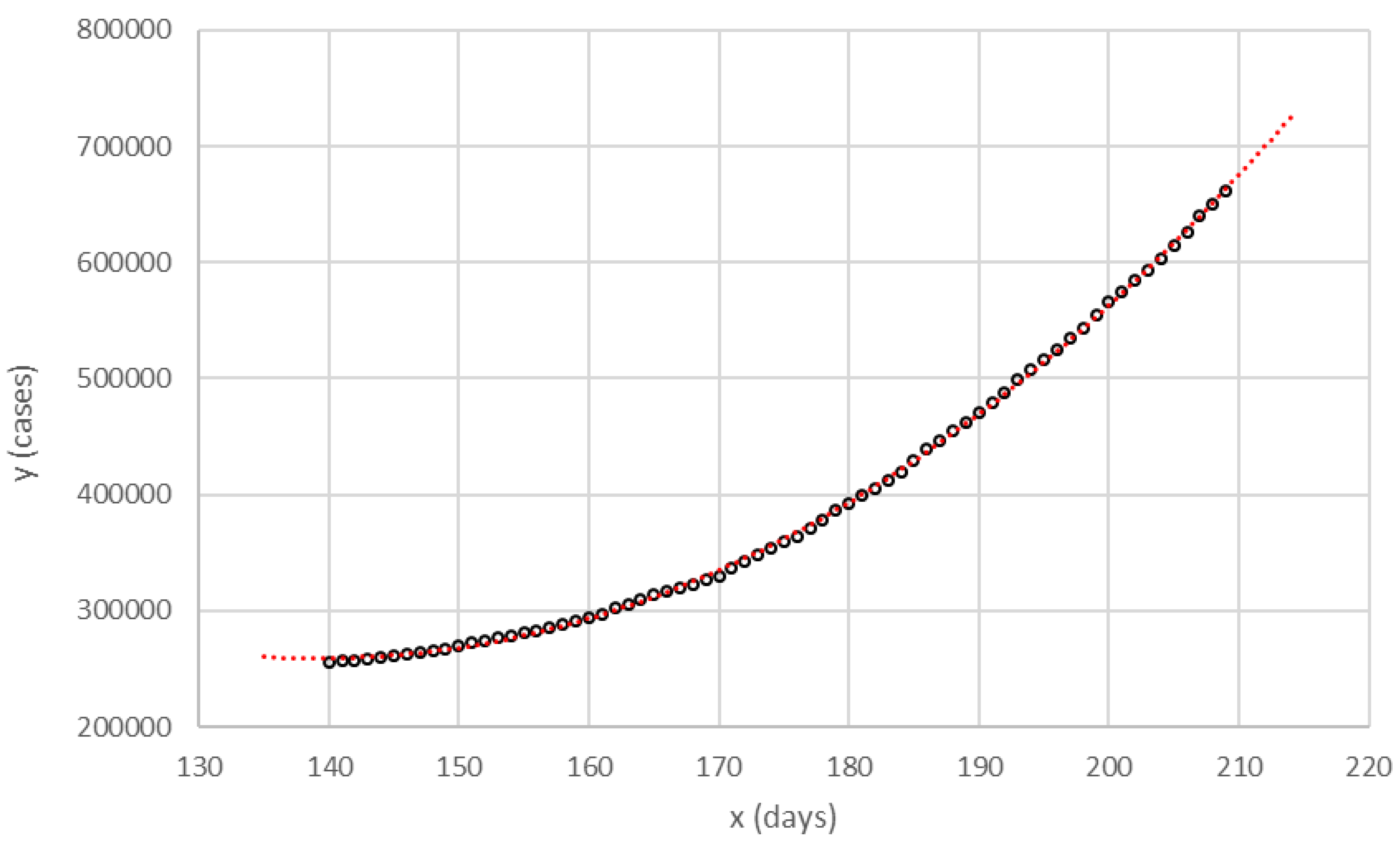
As an example of the facility of the cubic function to fit the pandemic curve (y), Figure 1 shows the fit with data from Spain between July 12 (x = 140) and September 19 (). The seventy values were adjusted to a cubic equation with , median relative error = 0.13%, and interquartile range (IQR) = 0.92%. The analytical curve in this figure is not a predictor, since it was obtained when all the information was already available on the corresponding dates, but shows a great facility of the cubic function to reproduce the cumulative number of cases on pandemic curve.
The analogy with kinematics equations and the ability to fit the epidemic curve suggest their use for forecasting. Equation (2) describes a rectilinear motion with a variable acceleration that increases or decreases linearly, since the acceleration equation is a line whose slope is . That is, Equation (2) ceases to be valid when there are increases or decreases in w that deviate from linearity. These deviations, in the case of an epidemic, are caused by NPIs that act either as obstacles that force a halt to the acceleration or, in the opposite direction, the acceleration will grow faster due to external factors such as the relaxation of restrictions on social distancing or mobility or climatic conditions.
Therefore, when using the cubic function to simulate the behavior of the pandemic, given that the factors that favor or hinder the spread depend on unpredictable political decisions and natural factors, the algorithm needs successive sections of cubic curves to deviate from the pattern of a linear relationship of acceleration with time, which is implicit in the third-order polynomial.
Hence, the algorithm variables are:
a. The number of days for which data of the cumulative number of cases fit a cubic equation. b. The criterion for discarding a section and calculating a new one. c. The relative error that determines the margin between favorable and unfavorable scenarios.
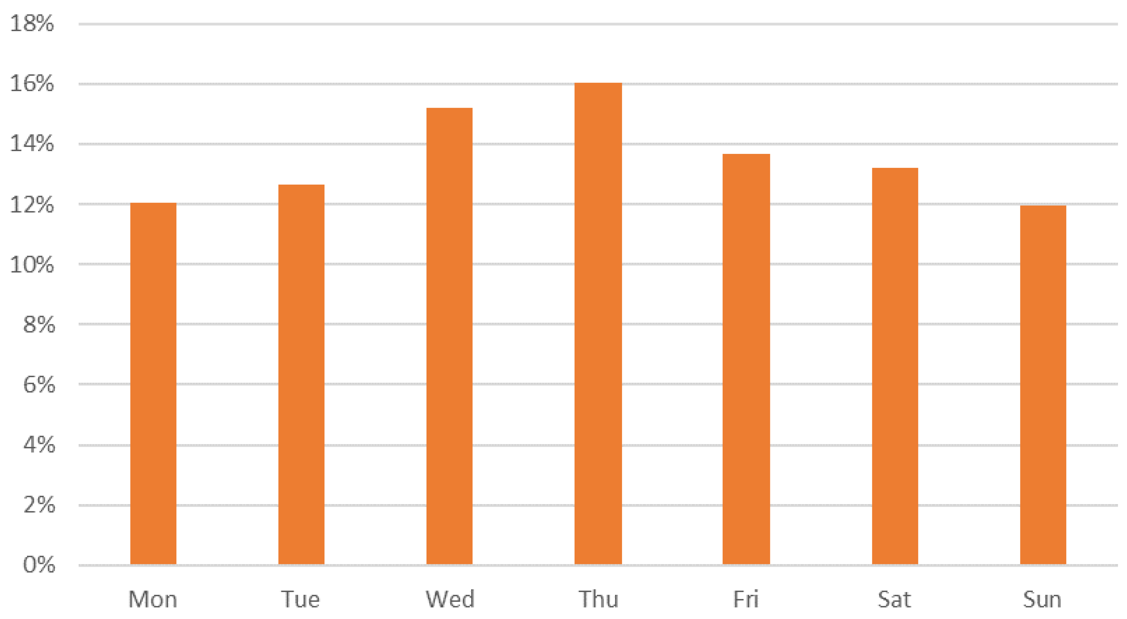
As can be seen in Figure 2, in Spain, there are biases in the daily values of cases depending on the day of the week. It can be observed that Wednesday (15.19%) and Thursday (16.03%) are the days with maximum values within the week, and Monday (12.03%) and Sunday (11.96%) are the days with a lower registration of cases. These biases are not related to the pandemic spread and are probably due to administrative problems in the case registration and notification process and perhaps also to fewer tests and diagnoses made on weekends. To avoid these biases that can negatively affect the predictive capacity of the algorithm, it is preferable that the algorithm works with the moving average of the cumulative number of cases of the last seven days (represented as ) instead of working with y values.
Indeed, the visual observation of the wave followed by new contagions detected along every week suggests the existence of measurement errors. The human resources employed to detect new contagions decrease on weekends, and the data flows at the beginning of the week include values that were buffered during the weekend, making Wednesday perhaps the “more standard day”. Measurement errors are minimized when averaging the seven days to complete a whole week.
Although this algorithm is still in the testing phase and, for now, it has only been tested with data from the cumulative number of cases from Spain between 1 June and 17 October, its variables were adjusted to obtain results with good approximations. The algorithm steps are as follows:
- 1.
- On day x, the first predictive equation is calculated, obtaining by linear regression the third-degree polynomial equation that best fits the values observed for the fourteen values between days () and (x). The coefficients of Equation (2), a, b, c, and d, are obtained. This equation is called the standard equation for day x.
- 2.
- From the standard equation forecast , the values for the days are projected. Two alternative predictions are calculated for a pandemic scenario that is worse and better than the standard prediction. These are called the unfavorable prediction and the favorable prediction, respectively. The calculation is performed by applying variations of to the standard prediction values. Therefore, a range [ - ] is defined. It is worth remarking that the limit is simply used to calculate the range that imposes the limit that, when trespassed, will require a re-estimation of the model.
- 3.
- 4.
- A new set of predictor equations is calculated in one of these situations:
- (a)
- One observed value is lower than those of the favorable prediction or exceeds the unfavorable prediction.
- (b)
- During 14 days, the observed values lie in the range [ - ].
- (c)
- One predicted value is less than the previous day, which denotes a maximum in the equation that would lead to the absurdity that the cumulative number of cases decreases.
- 5.
- The process is restarted in Step 1.
The range relative to the estimates does not represent a confidence interval for the prediction, but it is just used to represent favorable and unfavorable predictions relative to estimated values. The value was arbitrarily chosen, based solely on the empirical verification that with this margin, the value of the 14 day predictions does not differ excessively from the observed values. In this way, the margin is a sort of “rule-of-thumb” to re-calculate, if surpassed, a new arc of the cubic curve. It is intended to obtain a limited number of arcs of the epidemic curve that, in the context of the irregularity of the historical series of values, facilitate the qualitative understanding of the epidemic moment. This qualitative interpretation can probably be translated into an assessment of both the NPIs that are adopted at each moment and the influence of external factors that favor the spread. The “jumps” that occur between the different arcs of the predictor curve undoubtedly have a meaning, and we believe that it can be correlated with the favorable and unfavorable pandemic spreading factors.
The next section offers the results obtained by applying this algorithm to the official data of the of the pandemic’s second wave in Spain, until 17 October.
3. Data and Results
3.1. The Data
The historical data matrix used in this work was constructed from the daily data of the cumulative number of cases since the beginning of the pandemic, which are daily released by the Centre for the Coordination of Health Alerts and Emergencies of the Ministry of Health and correspond to the day prior to its publication. It is a set of 230 reports (until 19 October 2020) in pdf format, from which the daily values of the variable y were extracted. These reports can be found on the website of the Ministry of Health (https://www.mscbs.gob.es/), and one of them is referenced as an example [21]. As the Ministry has not provided information on weekends since July, the total cases corresponding to Fridays and Saturdays were obtained by linear interpolation between the values of Thursdays and Sundays.
The y value is defined by the Spanish Ministry of Health as “total cases confirmed by polymerase chain reaction test (PCR) until 10 May, and by PCR and IgM antibodies against SARS-CoV-2 (only if compatible symptoms) according to the new surveillance strategy” since 11 May. Therefore, in this study, all y values are confirmed cases by PCR or IgM compatible with symptoms. As explained in the previous section, the algorithm works with the moving average of total cumulative number of cases of seven days, represented as , that are directly calculated from the historical cumulative number of cases matrix. This value is related to the “Cumulative number for 7 days of COVID-19 cases per 100,000”, a rate usually used as an indicator, calculated as the number of new cases of disease in seven days multiplied by 100,000 and divided by the total number of individuals in the population at risk (CI 7d/100k).
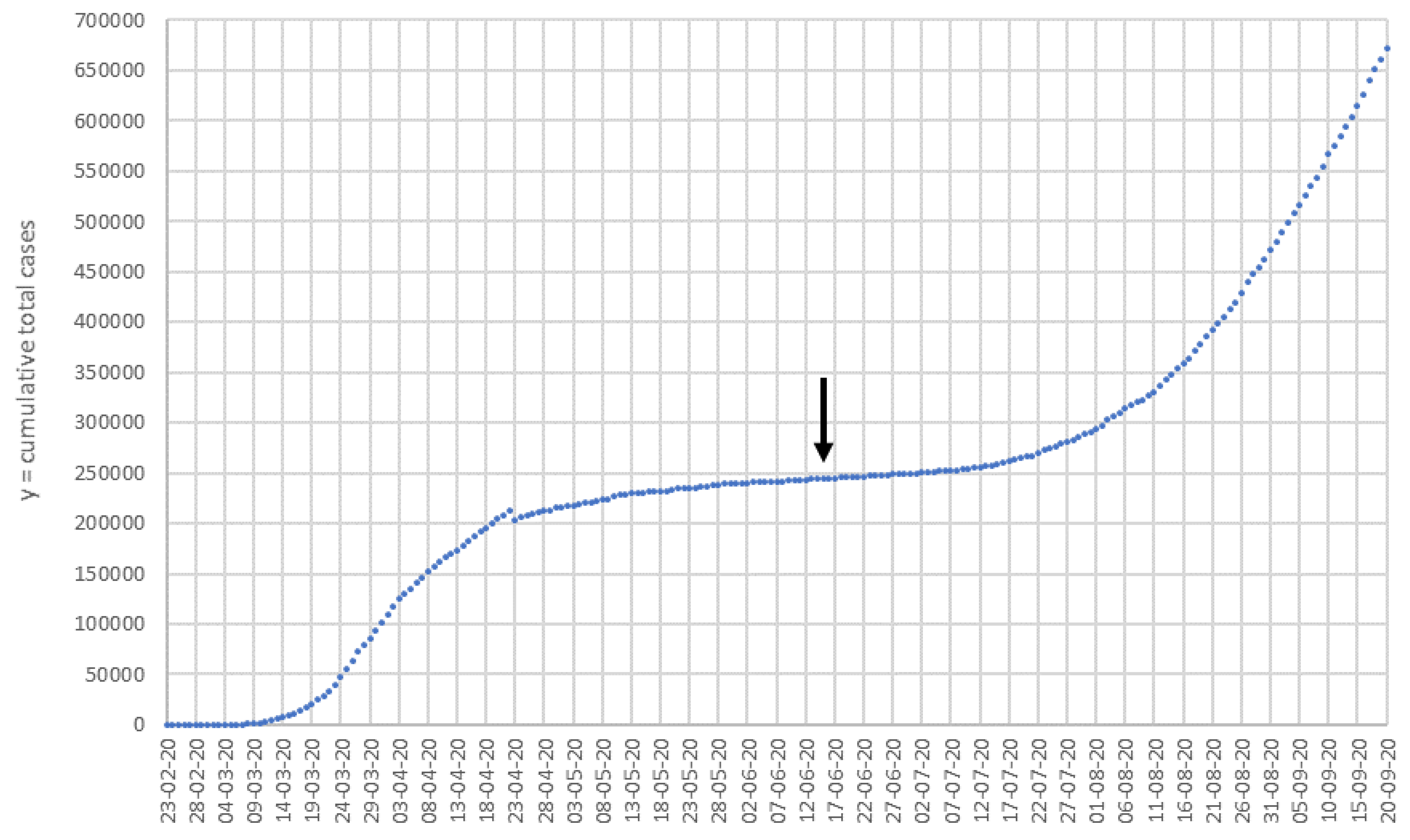
The theoretical border between the first and second pandemic wave was evaluated fitting y values from 16 May to 16 July, to a third-degree polynomial function () and setting the second derivative equal to zero, so 15 June is obtained as the inflection point. At this point, the curvature changes from convex to concave and marks hypothetically the end of the first wave and the start of the second (Figure 3). Thus, our study covers from 15 June, although it uses data from 14 days before to calculate the first of the predictive equations.
It is important to note that the information provided in Spain by the Ministry of Health has been the subject of controversy and criticism, being considered insufficient to understand the dynamics of COVID-19 and to take action, excluding ongoing retrospective series corrections [21].
3.2. Prediction Sections Obtained
The algorithm described previously was applied to the matrix obtaining a total of nine third-order function sections covering from 15 June to 18 October, as shown in Table 1.
The polynomial regressions are estimated for each sub-period using the standard least squares methodology. Hence, standard tests, such as the mean squared error or , are employed to measure the quality of fit for the estimations of the model obtained.
Equations (2)–(4) summarize the features of each section, indicating the days of duration of them, the range of the relative errors between and , the determination coefficient , the type of curvature, and the averages of the pandemic velocity v (cases/day) and acceleration w (cases/day2).
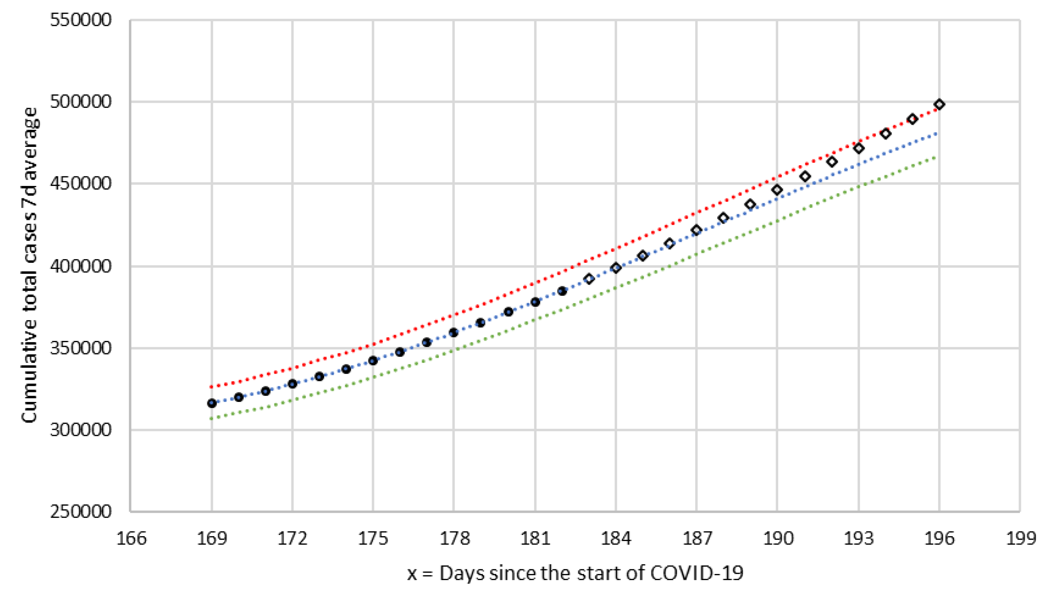
As an example, in Figure 4, the curves from section T-6 are represented. In this section, there exists a transition from positive to negative acceleration (from concavity to convexity) with an inflection point in x = 188 (28 August). The set of 14 values corresponding to the total number of cumulative number of cases from 10 August (x = 169) and 23 August (x = 182) was adjusted by linear regression to a cubic polynomial (), and from the equation, the three predictive curves were obtained: , , and (standard, favorable, and unfavorable). In order to compare the forecasts with the observed values, the values from August 24 were represented with a different symbol (rhombuses). In this section, it can be seen that they are located between the curves and until 6 September (x = 196), when the observed is higher than unfavorable forecast . According to the criteria established in the algorithm, on the day that the section is considered finished, three new predictor curves are calculated. Obviously, in the last observed point, the relative error exceeds the criterion value of and reaches a value of 3.30%, indicating the need for a new section.
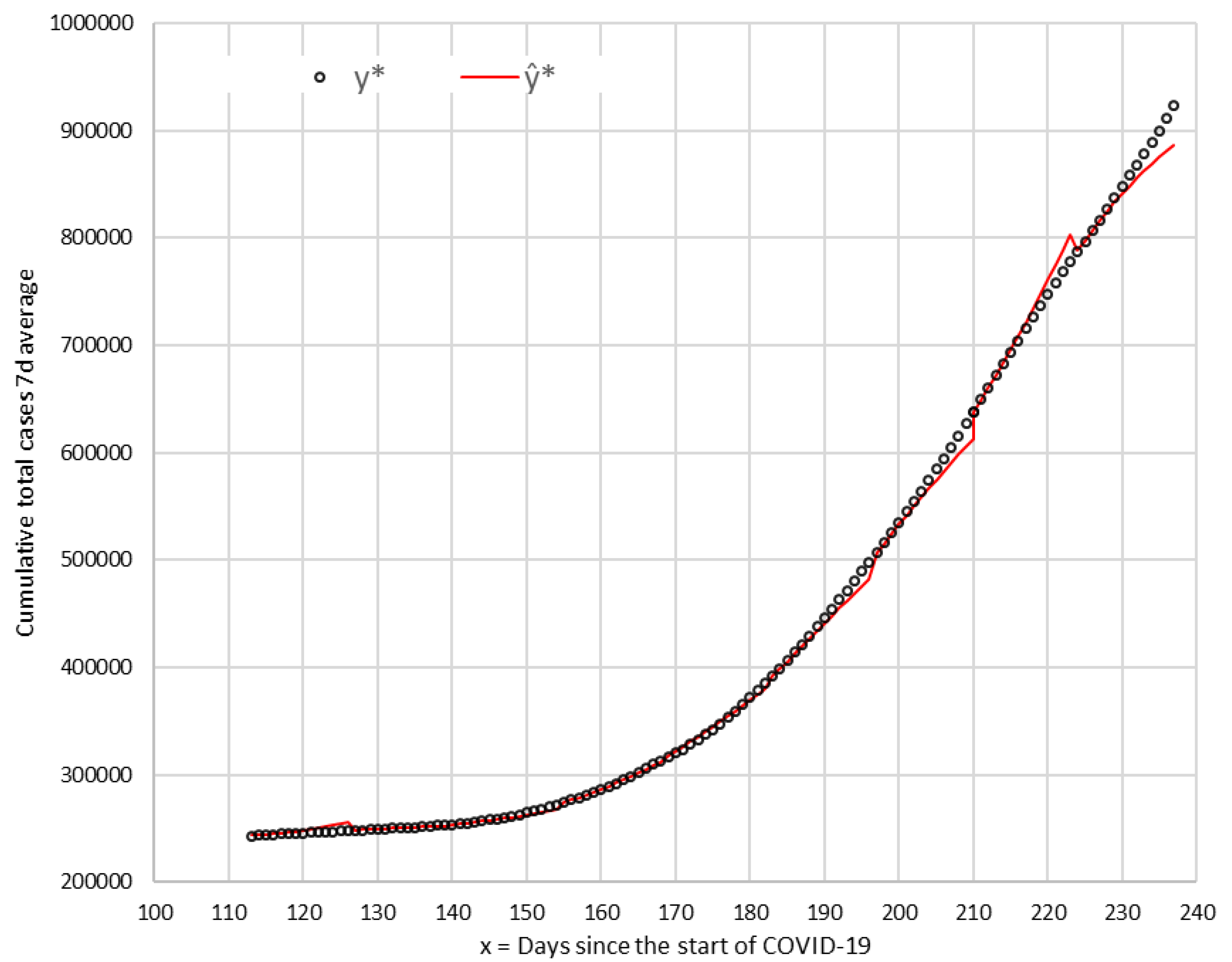
Figure 5 shows the arcs of the corresponding predictive curves () in the sections T-1 to T-9 together with the values of the total cumulative number of cases observed between 15 June and 17 October 2020.
All observed values are within the established range of (unfavorable—favorable), except five points (in T-1, T-6, T-7, T-8, and T-9), which are milestones of the algorithm, which indicates that a new forecast curve should be calculated. In the four sections (T-2, T-3, T-4, and T-5), all the points are within the range, and new curve sections are calculated due to the algorithm restriction to limit in 14 days each section.
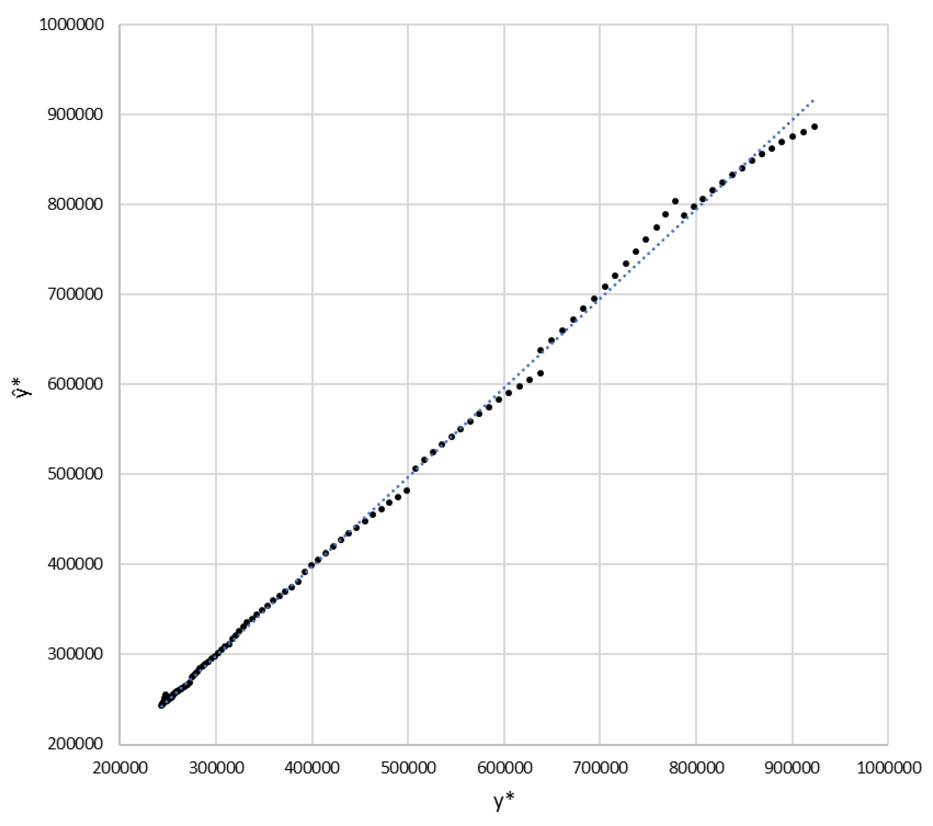
As an initial approach to the forecast quality, the coefficient of determination is used. The value of this coefficient for the arrays and is the set of the nine calculated predictive sections. This indicates a very high capacity of the algorithm to replicate, with an anticipation until two weeks, the observed results. In Figure 6, the values of are represented as a function of those of with very good correlation between both arrays: ( 0.9997).
As expected, in each of the sections of the predictive curves, increasing x increases the relative standard errors of prediction. This can be seen very well in Figure 7, where is plotted versus x. We also observed that between x = 127 (29 June) and x = 191 (1 September), the relative errors are in the range of −0.83% to 1.48%, and therefore, all the observed values fall between the favorable and unfavorable scenario. This fact will be interpreted later.
3.3. Nowcasting and Short-Term Forecasting Results
From the equations of each of the nine sections, the seven day forecasts and 14 day nowcasts/forecast were calculated.
In Table 2 and Table 3, these predictions are summarized by comparing them with the values observed on each date.
On the calculation day, the seven day forecasts predict the cumulative number of cases (seven day average) that will be recorded seven days later. At the same time, if we assume the hypothesis that there is a time lapse of 14 days between the infection and the cases’ registration, we also obtain an approximation of the cumulative number of infections (seven day average) that occurred one week ago. In turn, the 14 day forecasts predict the cumulative number of cases (seven day average) that will be registered 14 days later, and at the same time, a nowcast is obtained that is an approximation of the cumulative number of infections that are happening today. As the cumulative number of infections are very difficult to verify, the validation of the algorithm’s predictive capacity is evaluated by comparing the values of the cumulative number of cases (seven day average) observed seven and 14 days after the calculation date.
In Table 2, the seven day forecasts are presented. The relative error range is (−0.76%, 1.03%), and the median is −0.02. Clearly, all forecasts are inside the favorable-unfavorable scenarios margins ().
In Table 3, the 14 day forecasts are shown, and therefore, nowcasts are less accurate than seven day forecasts. The median of the relative errors is 1.15%, and the range is (−3.29%, 3.98%). Four of the nine 14 day forecasts lie within the margin between the favorable and unfavorable scenarios. In the other five predictions, the relative error does not in any case exceeded with respect to the standard prediction.
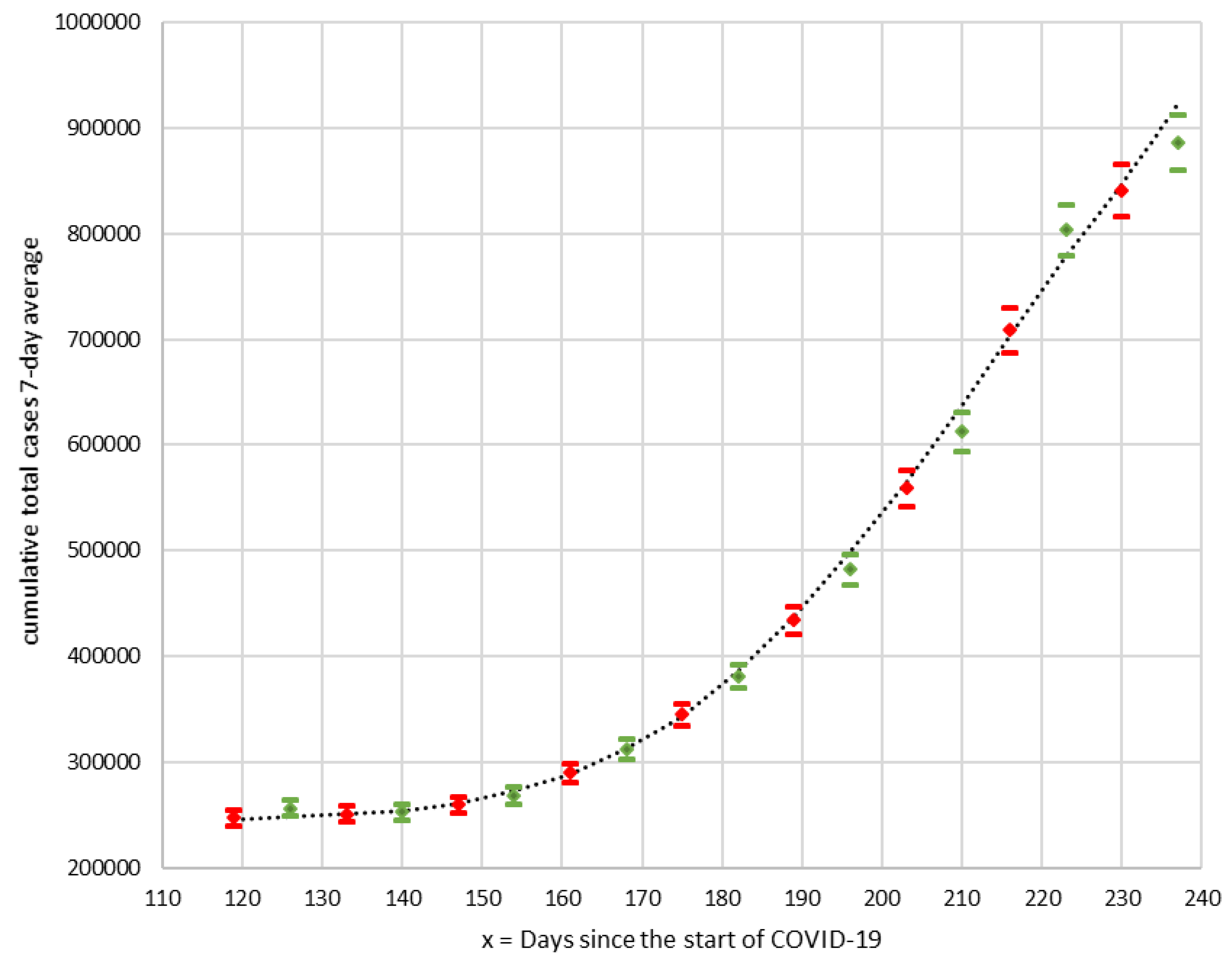
The results of seven and 14 day forecasts are represented in Figure 8, including the margins of the favorable and unfavorable scenarios, together with the observed curve of the seven day average of the cumulative number of cases.
4. Discussion
In this research, we show the adaptability of the cubic function to the epidemic curve of the cumulative number of cases, obtaining very good adjustments when applying it to the second wave of the COVID-19 pandemic in Spain.
The suitability of third and fourth degree equations for pandemic prediction has already been suggested in the literature. For example, the cubic function has been used for the prediction of mortality associated with COVID-19 because of its ability to reflect growth in the peak of daily cases [22,23] and has been tested, together with other equations, to predict the future development of the pandemic [24,25]. The approach that is described in this work is different, since, on the one hand, it does not intend to make long-term predictions, nor predict the peak nor the end of the pandemic, and on the other, a totally empirical approach to the problem is made, which avoids an epidemiological hypothesis. The objective is also different, since a nowcasting methodology is developed and tested that offers real-time approximations of the situation of the spread of infections, which can be of great value to adequately manage the pandemic.
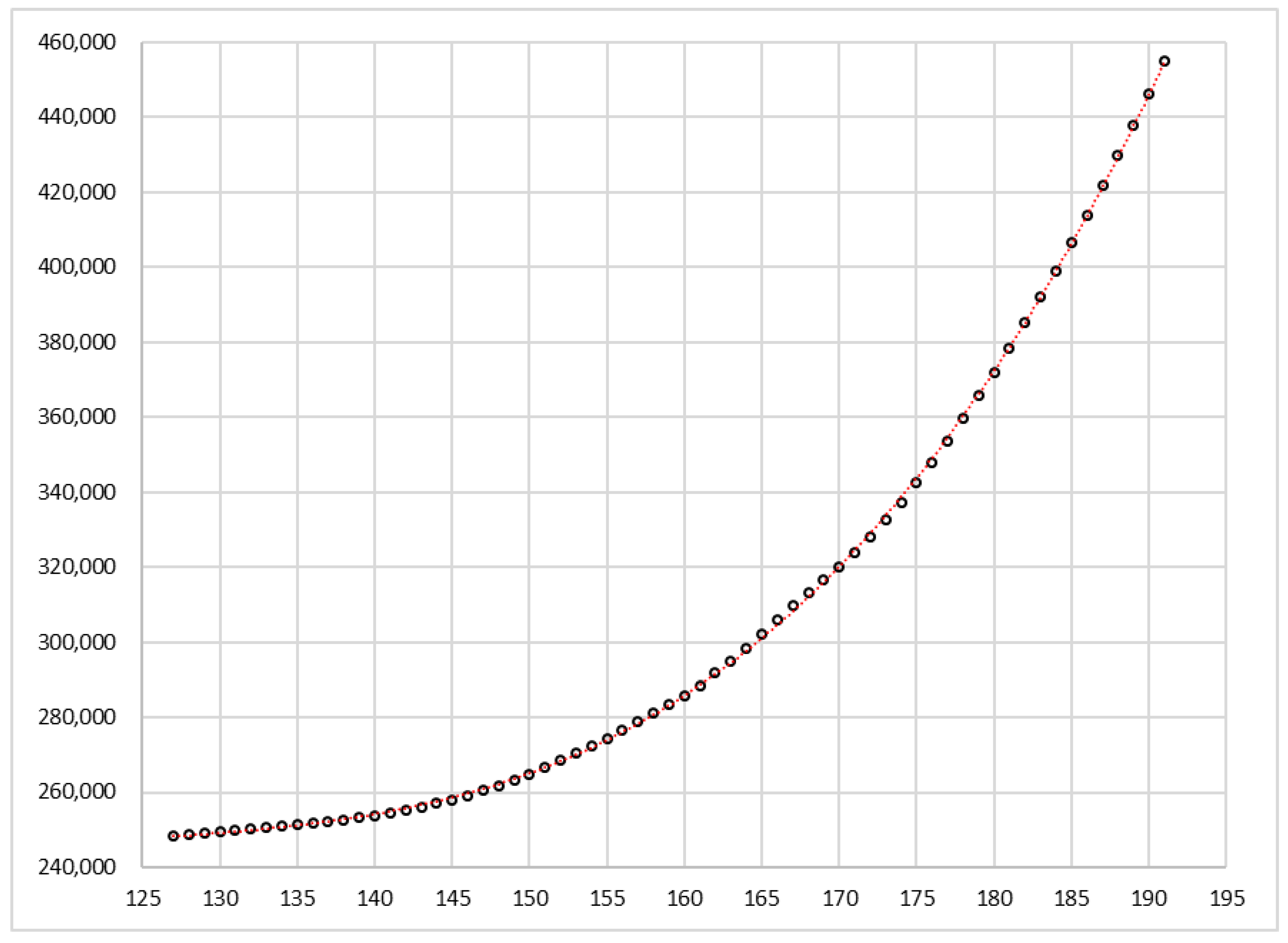
When the seven day average of the cumulative number of cases () is used as a variable, very good estimates are obtained with the cubic function for periods of up to two months. For 65 days, between 29 June (x = 127) and 1 September (x = 191), the values of in Spain fit almost perfectly the equation:
Essentially, the algorithm is a kinematic analogy that describes the space, velocity, and acceleration of a moving object with varying acceleration. The use of successive sections of the cubic curve is motivated by the similarity between the obstacles that slow down a moving body and the NPIs that are implemented to mitigate the propagation or the factors or circumstances that accelerate it, such as the increase of mobility or easing of previous interventions. An epidemic in which no type of intervention is adopted could probably be represented almost entirely by a third-degree equation, excluding the initial and final phases with asymptotic behavior. Therefore, the corrections that are made in the algorithm when a new curve section is calculated indicate that unfavorable circumstances are occurring or that the adopted NPIs are effective.
The results obtained in the predictions were satisfactory. The seven day predictions offer relative errors between −0.76% and 1.03% (all of them within the margins of the favorable-unfavorable scenarios). The 14 day predictions present relative errors between −3.29% and 3.98% (only four of them within the margins of the favorable-unfavorable scenarios). With the exception of seven of the observed values, the remaining 117 are within the range defined by the favorable and unfavorable predictions.
The most stable part of the curve reflected in Figure 9, between 29 June and 1 September, represents an accelerated growth without obstacles, so the values predicted by the curves of sections T-2 to T-6 have very low relative errors with respect to the observed values (between −0.83% and 1.48%). In this period, the acceleration grew linearly with a slope of 3.9 cases/day2, which caused the speed to multiply by 26 in just over two months (the seven day moving average of daily cases went from 326 to 8529). During this period in Spain, there was a notable absence of decisive interventions to stop the second wave, which is most likely reflected in the fact that the data fit the cubic equation very well. It was not until 20 August when the Spanish health authorities recognized that the situation was worrying: “… do not be fooled. If we still allow transmission to continue upwards, we will have many hospitalized, many admitted to the intensive care units (ICU), and many deceased”, declared the director of the Centre for Coordination of Health Alerts and Emergencies of the Spanish Ministry of Health [26].
The 14 day predictions are used as nowcasting to know in real time the evolution of infections. For this, the hypothesis was assumed that an average of 14 days elapse between infection and registration as a case of COVID-19. Although this is very approximate, it is possible to make a rough estimate of the delay time between the day of infection and the date of inclusion and publication as a confirmed case by the health authorities. For COVID-19, it was estimated by Lauer et al. [27] that the median incubation period is 5.1 days (95% CI, 4.5 to 5.8 days) and that less than 2.5% of infected people will present symptoms within 2.2 days (CI, 1.8 to 2.9 days) of exposure, while the onset of symptoms will appear in 11.5 days (CI, 8.2 to 15.6 days) for 97.5% of infected people. There is also a variable number of days of delay between the onset of symptoms until the date of registration as a confirmed case of COVID-19 by the health authorities and its inclusion in the epidemic statistics. In Spain, this delay, according to information from RENAVE(National Epidemiological Surveillance Network) [28], includes a median of two days (IQRs 1-4) from the onset of symptoms to consultation and a median of one day (IQRs 1-2) from consultation to diagnosis. There is no information on the delay between diagnosis and inclusion and data released by the Ministry, but it can be assumed that this delay should be about 1–2 days. Therefore, it is not risky to estimate an average total delay of about two weeks from infection to inclusion in official statistics.
Table 4 shows the information that would have been available applying the nowcast values obtained using the algorithm developed in this work.
On 28 June, the favorable nowcast indicated that the infections were controlled (the negative value makes no more sense than to indicate that in this scenario, there were no more new infections). However, the unfavorable scenario showed that more than three times more infections could be occurring than cases registered that day. Obviously, the nowcast shows a notable lack of definition about how the pandemic would evolve. However, two weeks later, the situation had changed, since both the favorable and unfavorable scenarios indicated that on 12 July, there were between 2.6 and 2.8 times more infections than the registered cases, and the 28 June unfavorable scenario was confirmed with more than 1000 new infections daily. These nowcasts clearly show the advisability of adopting restrictions and implementing NPIs, at least in the highest incidence geographic areas. On 26 July, the situation had notably worsened: the registered cases had multiplied by more than three, and there were between 2.3 and 2.4 times more infections than the registered cases. Many experts criticized the late reaction of central and regional authorities, the slowness of decision-making processes, and the low dependence on scientific advice [29].
On 6 September, the number of cases and the unfavorable nowcast indicated that pandemic spread had acquired a very high rate. However, between 19 September and 3 October, there were sudden changes in the immediate predictions, perhaps due to the confluence of negative factors (opening of schools) and positive factors (decreased mobility associated with holidays) together with the implementation of new NPIs.
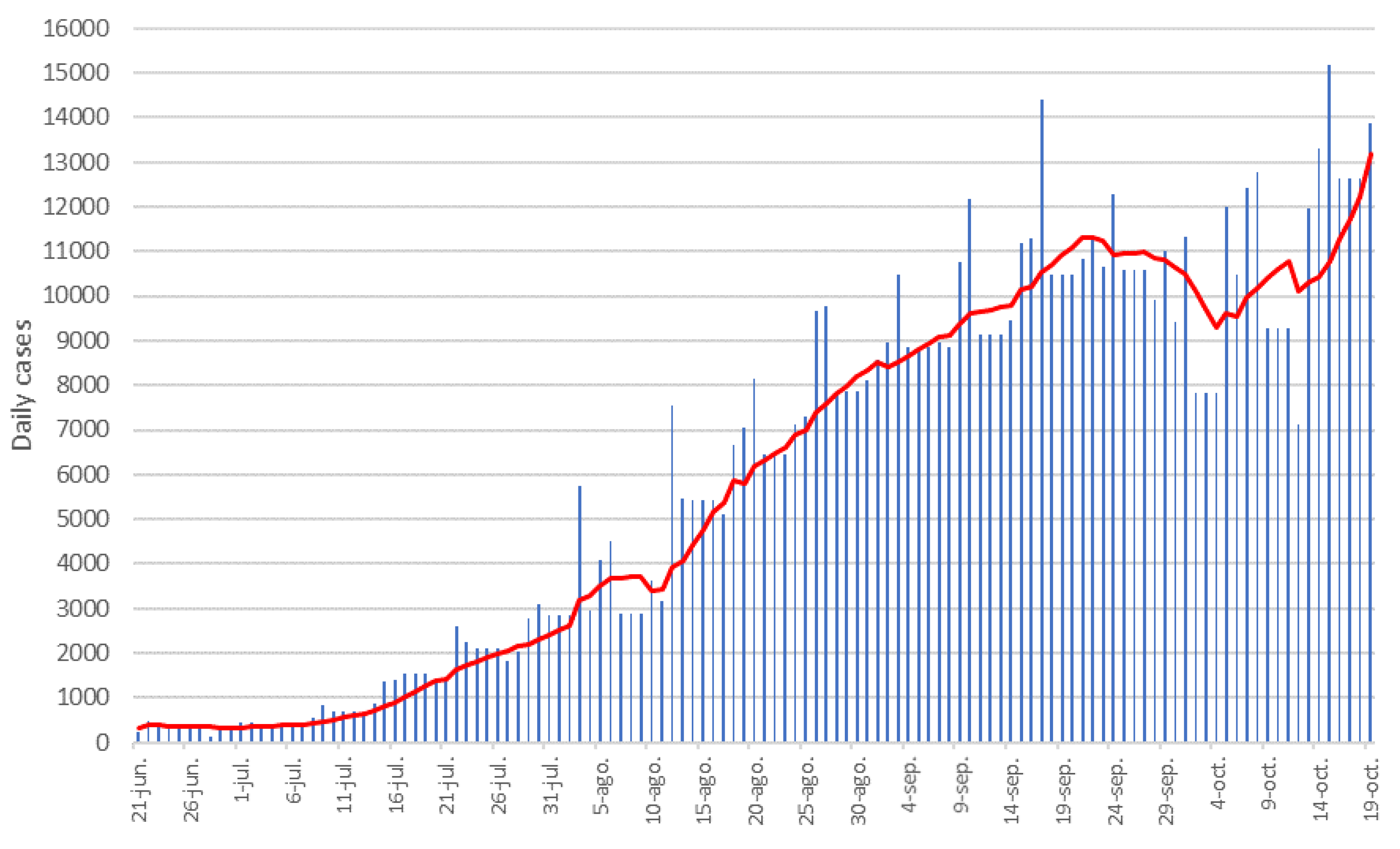
The irregularities shown by the nowcasts of 19 September and 3 October are a reflection of those that occur in the records of the cumulative number of cases that, at the time of writing this work, indicate an indefiniteness of trends, as can be observed in the epidemic curve of daily cases in Figure 10, with numerous irregularities since mid-September. It can be affirmed that the growing trend of infections began to slow down in the first half of September, which indicates that the curve began to flatten because the measures that began to be adopted at that time were effective; although, today, it cannot be known yet if they were sufficient.
To sum up, the developed nowcasting methodology is useful to anticipate the adoption of interventions. As was seen in the case of Spain, the nowcasts indicated very well the July dates in which the NPIs, that had relaxed greatly in the second half of June, should have been retaken. However, they did not begin to resume until the beginning of September, with greater effort and with less efficiency than if they had advanced to July.
When compared to alternative estimation methodologies, the algorithm provides similar numerical results to estimating rolling regressions, but our approach also provides the location of the negative and positive “jumps” that facilitate the understanding of the epidemiological moment and the need to undertake new measures.
In addition to the short-term forecast and nowcast capacity, the algorithm developed in this work has the potential for its simplicity and easy implementation, and at the same time, it can be useful in the public communication of the evolution of the pandemic, which is also an important NPI, to explain to the general public how the spread is taking place and why it is necessary to apply interventions that anticipate the dynamics of the pandemic.
Noticeably, this algorithm, which was developed during the second wave in Spain, must be readjusted to offer more accurate predictions and forecasts and must be tested with historical series from other countries to confirm its validity. Likewise, its predictive ability to project hospital needs and other epidemic parameters should also be tested.
Moreover, positive deviations from the estimated might indicate either a failure of the current containment efforts, while negative deviations might indicate a success in mitigation strategies.
Regarding the issue of the limitations associated with the significance of the results, in the field of forecasting, it is difficult to compute a test for the fitness of a model over a non-existing set of data. However, this difficulty grows in cases like the present one, since the evolution of COVID is determined by a multiplicity of factors, such as government intervention, external factors, such as weather, or even genetic factors. This makes it extremely difficult to use sample tests in this model. Nevertheless, we carried out sample tests weekly during the last month, and it worked fairly well. A good example to prove this is the small number of recalculations we needed to do when the actual data fall out of bounds.
5. Conclusions
It is observed that the epidemic curve of the cumulative number of COVID-19 cases fits adequately to a third-degree polynomial function for periods of up to two months with coefficients of determination greater than 0.97. This fact has been used as the basis for developing an algorithm that predicts the spread of the COVID-19 pandemic up to two weeks in advance.
The results obtained when testing this algorithm with the figures for the second pandemic wave in Spain, between 15 June and 17 October 2020, lead to short-term forecasts with relative errors of less than ±1.1 in the seven day predictions, all of them within the favorable-unfavorable scenarios defined.
The relative errors of 14 day predictions are less than and, only in four of them, within the favorable-unfavorable scenarios previously defined.
To avoid the bias observed in Spain depending on the day of the week in the values of published daily cases, the seven day moving averages of the cumulative number of cases were used. The use of this variable leads to more accurate predictions than the daily values of the cumulative number of cases and allows the predictions of two epidemiological indicators that are being widely used in many countries: seven day and 14 day notification rate of new COVID-19 cases per 100,000 inhabitants.
The 14 day predictions are used as nowcasting to know in real time the evolution of infections. For this, the hypothesis is that, on average, it must be assumed that 14 days elapse between infection and registration as a COVID-19 case. This information is of great practical value for the correct management of the pandemic.
One of the most relevant contributions of this work is, perhaps, the nowcasting of the daily “unobserved” infections, assessed by means of estimating the detections that will occur in 14 days, which serve as a nowcast of today’s infections. In this sense, if a rolling calculation had been used, many more predictive values would have been obtained, but for the days in which 14 day prediction of detections were calculated in this work, the results would have been the same. Furthermore, to interpret the “jumps” between the different arcs of the cubic curve, their number has to be limited, which leads to a model similar to the one used here. Therefore, although it is not the usual procedure, the results are similar to those that would be obtained using a rolling regression, while obtaining, at the same time, the location of the “jumps”.
The results obtained suggest that the algorithm developed can be used to know in real time the dynamics of the spread of the pandemic and to be able to adopt NPIs at the right time and properly prepare the health system. Nevertheless, the algorithm will be assayed and can be improved by studying other COVID-19 historical series.
Author Contributions
All authors contributed equally to this work. All authors read and agreed to the published version of the manuscript.
Funding
This work was supported by the AEI/Ministerio de Economía, Industria y Competitividad (MINEIC) and FEDER Project ECO2017-83255-C3-3-P and the Generalitat Valenciana (PROMETEO/2018/102 and GV/2017/052). The authors also acknowledge the support from the “Betelgeux-Christeyns” Chair for Sustainable Economic Development. This paper is part of the research thematic network ECO2016-81901-REDT financed by MINEIC. The usual disclaimer applies.
Institutional Review Board Statement
Not applicable.
Informed Consent Statement
Not applicable.
Data Availability Statement
Data available on request from the authors.
Acknowledgments
We thank the Editor and three anonymous reviewers for their helpful comments on earlier drafts of the manuscript.
Conflicts of Interest
The authors declare no conflict of interest.
References
- Giráldez, F. Por qué los Humanos no Entendimos lo que Estaba Pasando? Available online: comunidaddeloslibros.com (accessed on 20 November 2020).
- BMJ. BMJ Newsroom: UK’s Response to Covid-19 “Too Little, Too Late, Too Flawed”, 15/15/2020; BMJ: London, UK, 2020. [Google Scholar]
- Silv, M. COVID-19: Too little, too late? Lancet 2020, 395, 755. [Google Scholar] [CrossRef]
- MSF. Poco, Tarde y Mal. El Inaceptable Desamparo de Las Personas Mayores en Las Residencias Durante la COVID-19 en España; Technical Report; Médicos Sin Fronteras: Geneva, Switzerland, 2020. [Google Scholar]
- Johns Hopkins University of Medicine. Animated Maps—Johns Hopkins Coronavirus Resource Center; Johns Hopkins University of Medicine: Baltimore, MD, USA, 2020. [Google Scholar]
- Nicola, M.; Alsafi, Z.; Sohrabi, C.; Kerwan, A.; Al-Jabir, A.; Iosifidis, C.; Agha, M.; Agha, R. The socio-economic implications of the coronavirus pandemic (COVID-19): A review. Int. J. Surg. 2020, 78, 185–193. [Google Scholar] [CrossRef] [PubMed]
- Baldwin, R.; Mauro, B.W.D. Economics in the Time of COVID-19; Centre for Econnomic Policy Research Press: London, UK, 2020; pp. 105–109. [Google Scholar]
- Eurostat. GDP and Employment Flash Estimates for the Second Quarter of 2020: GDP Down by 12.1% and Employment Down by 2.8% in the Euro Area—Product—Eurostat; Eurostat: Luxembourg, 2020. [Google Scholar]
- Sachs, J.; Schmidt-Traub, G.; Kroll, C.; Lafortune, G.; Fuller, G.; Woelm, F. The Sustainable Development Report. The Sustainable Development Goals and COVID-19; Technical Report; Cambridge University Press: Cambridge, UK, 2020. [Google Scholar]
- Sachs, J.D.; Abdool Karim, S.; Aknin, L.; Allen, J.; Brosbøl, K.; Cuevas Barron, G.; Daszak, P.; Espinosa, M.F.; Gaspar, V.; Gaviria, A.; et al. Lancet COVID-19 Commission Statement on the occasion of the 75th session of the UN General Assembly. Lancet 2020, 396, 1102–1124. [Google Scholar] [CrossRef]
- Matrajt, L.; Leung, T. Evaluating the Effectiveness of Social Distancing Interventions to Delay or Flatten the Epidemic Curve of Coronavirus Disease. Emerg. Infect. Dis. 2020, 26, 1740–1748. [Google Scholar] [CrossRef]
- Chaccour, C. COVID-19: Five Contrasting Public Health Responses to the Epidemic. Available online: https://www.isglobal.org/ (accessed on 17 March 2020).
- Lai, S.; Ruktanonchai, N.W.; Zhou, L.; Prosper, O.; Luo, W.; Floyd, J.R.; Wesolowski, A.; Santillana, M.; Zhang, C.; Du, X.; et al. Effect of non-pharmaceutical interventions to contain COVID-19 in China. Nature 2020, 585, 410–413. [Google Scholar] [CrossRef]
- Orea, L.; Álvarez, I.C. How effective has the Spanish lockdown been to battle COVID-19? A spatial analysis of the coronavirus propagation across provinces. Available online: https://navarra.opennemas.com/media/navarra/files/2020/04/16/dt2020-03.pdf (accessed on 30 December 2020).
- Bank of England. Central Bank Digital Currency. Opportunities, Challenges and Design; Technical Report March; Bank of England: London, UK, 2020. [Google Scholar]
- Schmid, F.; Wang, Y.; Harou, A. Arcimís: Guías Generales Para la Predicción Inmediata: Resumen; Technical Report; AEMET: Madrid, Spain, 2019.
- Kapetanios, G.; Papailias, F. Big Data & Macroeconomic Nowcasting: Methodological Review. In Economic Statistics Centre of Excellence (ESCoE) Discussion Papers; ESCoE: London, UK, 2018. [Google Scholar]
- Bregler, C. Kinematic Motion Models. In Computer Vision; Ikeuchi, K., Ed.; Springer: Boston, MA, USA, 2014; pp. 437–440. [Google Scholar] [CrossRef]
- Vazquez, A. Polynomial Growth in Branching Processes with Diverging Reproductive Number. Phys. Rev. Lett. 2006, 96, 038702. [Google Scholar] [CrossRef] [Green Version]
- Susser, M.; Adelstein, A. An introduction to the work of William Farr. Am. J. Epidemiol. 1975, 101, 469–476. [Google Scholar] [CrossRef]
- Centro de Coordinación de Alertas y Emergencias Sanitarias. Actualización n° 1 a 211. Enfermedad Por el Coronavirus (COVID-19); Centro de Coordinación de Alertas y Emergencias Sanitarias: Madrid, Spain, 2020. [Google Scholar]
- Gerli, A.; Centanni, S.; Miozzo, M.; Sotgiu, G. Predictive models for COVID-19-related deaths and infections. Int. J. Tuberc. Lung Dis. 2020, 24, 647–650. [Google Scholar] [CrossRef]
- Sotgiu, G.; Gerli, A.G.; Centanni, S.; Miozzo, M.; Canonica, G.W.; Soriano, J.B.; Virchow, J.C. Advanced forecasting of SARS-CoV-2-related deaths in Italy, Germany, Spain, and New York State. Allergy 2020, 75, 1813–1815. [Google Scholar] [CrossRef]
- Akhtar, I.U.H. Understanding the CoVID-19 pandemic Curve through statistical approach. medRxiv 2020. [Google Scholar] [CrossRef]
- Amar, L.A.; Taha, A.A.; Mohamed, M.Y. Prediction of the final size for COVID-19 epidemic using machine learning: A case study of Egypt. Infect. Dis. Model. 2020, 5, 622–634. [Google Scholar] [CrossRef]
- Fernando Simón Enciende la Alarma: “Las Cosas No Van Bien. Está Fuera de Control en Algunos Puntos”. Available online: https://www.elespanol.com/ (accessed on 20 August 2020).
- Lauer, S.A.; Grantz, K.H.; Bi, Q.; Jones, F.K.; Zheng, Q.; Meredith, H.R.; Azman, A.S.; Reich, N.G.; Lessler, J. The Incubation Period of Coronavirus Disease 2019 (COVID-19) From Publicly Reported Confirmed Cases: Estimation and Application. Ann. Intern. Med. 2020, 172, 577–582. [Google Scholar] [CrossRef] [Green Version]
- Equipo COVID-19. Situación de COVID-19 en España a 16 de Septiembre de 2020, Equipo Covid-19 and RENAVE. Available online: https://www.isciii.es/QueHacemos/Servicios/VigilanciaSaludPublicaRENAVE/EnfermedadesTransmisibles/Paginas/InformesCOVID-19.aspx (accessed on 16 September 2020).
- García-Basteiro, A.; Alvarez-Dardet, C.; Arenas, A.; Bengoa, R.; Borrell, C.; Del Val, M.; Franco, M.; Gea-Sánchez, M.; Otero, J.J.G.; Valcárcel, B.G.L.; et al. The need for an independent evaluation of the COVID-19 response in Spain. Lancet 2020. [Google Scholar] [CrossRef]
Figure 1.
Second pandemic wave in Spain: fit by linear regression of the observed cumulative number of cases to a third-degree polynomial, 16,584x + 1,524,253 (red curve), from 12 July () to 19 September ().
Figure 1.
Second pandemic wave in Spain: fit by linear regression of the observed cumulative number of cases to a third-degree polynomial, 16,584x + 1,524,253 (red curve), from 12 July () to 19 September ().

Figure 2.
Percentages of daily cases out of total weekly cases on each day of the week. Nineteen week averages between 1 June and 11 October (Spain).
Figure 2.
Percentages of daily cases out of total weekly cases on each day of the week. Nineteen week averages between 1 June and 11 October (Spain).

Figure 3.
Cumulative number of cases in Spain from 23 February until 20 September. The arrow marks an inflection point at 15 June, which theoretically separates the two pandemic waves. Data source: Centro de Coordinación de Alertas y Emergencias Sanitarias (CCAES).
Figure 3.
Cumulative number of cases in Spain from 23 February until 20 September. The arrow marks an inflection point at 15 June, which theoretically separates the two pandemic waves. Data source: Centro de Coordinación de Alertas y Emergencias Sanitarias (CCAES).

Figure 4.
T-6 predictive segment calculated on 23 August between 10 and 23 August (x = 169 to 182). The black circles represent the 14 values used to obtain the curve by linear regression. The rhombuses are the observed values since 24 August. The and curves were obtained by increasing and reducing the values of by 3%. The standard equation: 2061.89 380,298.77 23,354,382.14; .

Figure 5.
Predictive arcs (red line) calculated from 15 June (x = 113) to 17 October (x = 237). The black circles represent all the observed values of cumulative number of cases for a seven day average.
Figure 5.
Predictive arcs (red line) calculated from 15 June (x = 113) to 17 October (x = 237). The black circles represent all the observed values of cumulative number of cases for a seven day average.

Figure 6.
Arrays of observed and forecasted values between 15 June and 17 October ( vs. ).

Figure 7.
Relative standard errors for each of the nine predictor curves.

Figure 8.
Favorable and unfavorable scenarios versus observed curve of the seven day average of the cumulative number of cases: (dashed line), 14 days (green), and seven days (red).
Figure 8.
Favorable and unfavorable scenarios versus observed curve of the seven day average of the cumulative number of cases: (dashed line), 14 days (green), and seven days (red).

Figure 9.
Seven day average estimation between 29 June and 2 September.

Figure 10.
Daily cases and seven day moving average (red lines).


Table 1.
Characteristics of the sections of the standard prediction, using arcs of cubic curves, indicating for each one the date on which it was constructed, the duration in days, the relative error () range, the coefficient of determination (), the curvature, the average velocity of propagation (v), and the average acceleration (w).
| Section | Date | Days | Min | Max | Curvature | vAverage | wAverage | |
|---|---|---|---|---|---|---|---|---|
| T-1 | 14 June | 14 | −3.21% | −0.05% | 0.9728 | CONCAVE | 968 | 94.4 |
| T-2 | 28 June | 14 | −0.05% | 0.39% | 0.9880 | CONVEX | 346 | −3.7 |
| T-3 | 12 July | 14 | 0.00% | 1.38% | 0.9994 | CONCAVE | 1082 | 72.7 |
| T-4 | 26 July | 14 | −0.37% | 0.38% | 0.9984 | CONCAVE | 2892 | 106.6 |
| T-5 | 9 August | 14 | −0.83% | 1.15% | 0.9966 | CONCAVE | 4846 | 90.7 |
| T-6 | 23 August | 14 | 0.03% | 3.30% | 0.9984 | CONCAVE-CONVEX | 6893 | −35.4 |
| T-7 | 6 September | 13 | 0.08% | 3.38% | 0.9965 | CONVEX | 8078 | −136.8 |
| T-8 | 19 September | 14 | −3.29% | 0.06% | 0.9970 | CONCAVE | 12,785 | 276.7 |
| T-9 | 3 October | 13 | −0.08% | 3.31% | 0.9937 | CONVEX | 7734 | −219.9 |
Table 2.
Seven day forecasts.
| Section | Calculation Day | Forecast For: | |||
|---|---|---|---|---|---|
| T-1 | 14 June | 21 June | 247,367 | 245,510 | −0.76% |
| T-2 | 28 June | 5 July | 250,586 | 250,529 | −0.02% |
| T-3 | 12 July | 19 July | 259,508 | 260,450 | 0.36% |
| T-4 | 26 July | 2 August | 289,618 | 288,548 | −0.37% |
| T-5 | 9 August | 16 August | 344,827 | 342,503 | −0.68% |
| T-6 | 23 August | 30 August | 434,097 | 438,028 | 0.90% |
| T-7 | 6 September | 13 September | 558,756 | 564,592 | 1.03% |
| T-8 | 19 September | 26 September | 708,587 | 704,672 | −0.56% |
| T-9 | 3 October | 10 October | 841,119 | 847,748 | 0.78% |
Table 3.
Fourteen day forecasts/nowcasts.
| Section | Calculation Day | Forecast For: | |||
|---|---|---|---|---|---|
| T-1 | 14 June | 28 June | 256,043 | 248,069 | −3.21% |
| T-2 | 28 June | 12 July | 252,933 | 253,917 | 0.39% |
| T-3 | 12 July | 26 July | 268,568 | 272,331 | 1.38% |
| T-4 | 26 July | 9 August | 312,108 | 313,303 | 0.38% |
| T-5 | 9 August | 23 August | 380,721 | 385,135 | 1.15% |
| T-6 | 23 August | 6 September | 481,845 | 498,302 | 3.30% |
| T-7 | 6 September | 20 September | 612,775 | 638,020 | 3.96% |
| T-8 | 19 September | 3 October | 803,787 | 778,216 | −3.29% |
| T-9 | 3 October | 17 October | 886,367 | 923,150 | 3.98% |
Table 4.
Nowcast estimations.
| Date | Observed Cumulative Cases | Nowcasts Cumulative Infections | ||
|---|---|---|---|---|
| Cumulative Number of Cases | Average 14d Daily Cases | Favorable- Unfavorable | Average 14 Days Daily Infections | |
| 28 June 2020 | 248,069 | 354 | 245,345–260,450 | −215–1238 |
| 12 July 2020 | 253,917 | 418 | 260,511–276,626 | 1083–1150 |
| 26 July 2020 | 272,331 | 1315 | 302,745–321,471 | 3017–3203 |
| 9 August 2020 | 313,303 | 2927 | 369,300–392,143 | 4754–5048 |
| 23 August 2020 | 385,135 | 5131 | 467,390–496,301 | 7006–7440 |
| 6 September 2020 | 498,302 | 8083 | 594,392–631,159 | 7007–9633 |
| 19 September 2020 | 626,918 | 9187 | 779,674–827,901 | 13,723–14,572 |
| 3 October 2020 | 778,216 | 10,807 | 859,776–912,958 | 6810–7232 |
Publisher’s Note: MDPI stays neutral with regard to jurisdictional claims in published maps and institutional affiliations. |
© 2021 by the authors. Licensee MDPI, Basel, Switzerland. This article is an open access article distributed under the terms and conditions of the Creative Commons Attribution (CC BY) license (http://creativecommons.org/licenses/by/4.0/).
Share and Cite
MDPI and ACS Style
Orihuel, E.; Sapena, J.; Navarro-Ortiz, J. An Empirical Algorithm for COVID-19 Nowcasting and Short-Term Forecast in Spain: A Kinematic Approach. Appl. Syst. Innov. 2021, 4, 2. https://0-doi-org.brum.beds.ac.uk/10.3390/asi4010002
AMA Style
Orihuel E, Sapena J, Navarro-Ortiz J. An Empirical Algorithm for COVID-19 Nowcasting and Short-Term Forecast in Spain: A Kinematic Approach. Applied System Innovation. 2021; 4(1):2. https://0-doi-org.brum.beds.ac.uk/10.3390/asi4010002
Chicago/Turabian StyleOrihuel, Enrique, Juan Sapena, and Josep Navarro-Ortiz. 2021. "An Empirical Algorithm for COVID-19 Nowcasting and Short-Term Forecast in Spain: A Kinematic Approach" Applied System Innovation 4, no. 1: 2. https://0-doi-org.brum.beds.ac.uk/10.3390/asi4010002