Transient Thermo-Mechanical Analysis of Steel Ladle Refractory Linings Using Mechanical Homogenization Approach


LaMé laboratory (EA 7494), Université d’Orléans, Université de Tours, INSA Centre Val de Loire, 8 rue Léonard de Vinci, 45072 Orléans, France
*
Authors to whom correspondence should be addressed.
Ceramics 2020, 3(2), 171-189; https://0-doi-org.brum.beds.ac.uk/10.3390/ceramics3020016
Submission received: 18 February 2020
/
Revised: 13 March 2020
/
Accepted: 18 March 2020
/
Published: 2 April 2020
(This article belongs to the Special Issue Design, Properties, Damage and Lifetime of Refractory Ceramics)
Abstract
:Mortarless refractory masonry structures are widely used in the steel industry for the linings of many high-temperature industrial applications including steel ladles. The design and optimization of these components require accurate numerical models that consider the presence of joints, as well as joint closure and opening due to cyclic heating and cooling. The present work reports on the formulation, numerical implementation, validation, and application of homogenized numerical models for the simulation of refractory masonry structures with dry joints. The validated constitutive model has been used to simulate a steel ladle and analyze its transient thermomechanical behavior during a typical thermal cycle of a steel ladle. A 3D solution domain and enhanced thermal and mechanical boundary conditions have been used. Parametric studies to investigate the impact of joint thickness on the thermomechanical response of the ladle have been carried out. The results clearly demonstrate that the thermomechanical behavior of mortarless masonry is orthotropic and nonlinear due to the gradual closure and reopening of the joints with the increase and decrease in temperature. In addition, resulting thermal stresses increase with the increase in temperature and decrease with the increase in joint thickness.
1. Introduction
Steel ladles are industrial vessels that are used in the steel industry for liquid steel transportation and refinement. Normal operating conditions of steel ladles include high operating temperatures (around 1700 °C), high thermal stresses, slag corrosion, and degradation of layers in contact with liquid steel. To withstand these severe operating conditions, steel ladle design is based on the concept of multi-layer design. Each layer has unique thermal, mechanical, physical, and chemical properties. The most critical layer in the steel ladle is the working lining layer in contact with liquid steel, as its temperature values are the highest within the ladle. In addition, this layer is usually subjected to thermal shock and a severe chemical environment, leading to thermomechanical degradation [1].
Generally, working linings are made of refractory masonry bricks separated by small gaps (also called dry joints). Often, these gaps result from the surface roughness of the bricks, brick dimensions, and shape errors during manufacturing. However, sometimes, for instance, in blast furnaces, the initial gaps are designed and obtained using cardboard blocks during the installation of masonry to compensate for thermal expansion effects. Indeed, many studies have shown that joints have a great impact on the overall thermomechanical response of mortarless refractory masonry (working lining) [2,3] as they allow the bricks to expand freely (until closure of joints), resulting in lower values of compressive stresses; then, after closure of the joints, compressive stresses increase at a higher rate [4,5].
The design and optimization of steel ladles require accurate thermal and mechanical numerical models with proper boundary conditions and solution domains. Most previous studies typically focused on studying the thermal and heat transfer behavior of steel ladles during the steel making process. For instance, Xia and Ahokainen [6] numerically analyzed the impact of preheating temperature and slag heat losses on thermal stratification in a steel ladle during the holding step. Similarly, Glaser et al. [7] developed a 2D axisymmetric numerical model to investigate heat transfer behavior and heat losses during the liquid steel teeming step. Recently, Santos et al. [8] presented a 2D axisymmetric transient thermal numerical model to investigate the impact of lining design on the transient thermal behavior and energy consumption of a steel ladle during preheating, holding liquid steel, and being empty.
With regard to the thermomechanical modelling of steel ladles, few studies have been carried out. All the bricks and joints of the working lining, as well as the contact between them, lead to an increase in the computational time and cost. Furthermore, a converged solution (accurate solution) of the computations is not guaranteed. For these reasons, a number of authors have neglected the presence of joints [9], while others have considered only a few bricks and joints between them [10]. For example, Yilmaz used a 2D steady-state axisymmetric finite element simulation to investigate the thermomechanical response of a ladle. The presence of joints within the working lining and bottom has been neglected and all lining layers have been considered isotropic. Aidong et al. [10] investigated the influence of material properties and lining thickness on the thermomechanical behavior of the slag zone using 2D transient finite element analysis of a few bricks in the slag line zone and Taguchi method. Due to the selected 2D solution domain, only one head joint with 0.4 mm thickness has been considered while bed joints have been neglected.
A reasonable approach to consider the presence of joints and their impact on the thermomechanical response of mortarless masonry without increasing computation costs is to replace the bricks and joints by an equivalent material. Nguyen et al. [4] developed and validated a homogeneous equivalent material model of a mortarless refractory masonry structure. This model is based on four joint patterns, as well as transition criteria between them. The model considers the influence of the closure of joints on the thermomechanical response. Gasser et al. [11] used this model and developed steady-state 3D finite element models of a steel ladle to investigate the influence of bottom design (radial, parallel, and fishbone designs) and joint thickness on the resulting thermomechanical stresses. Joints in the ladle bottom have been considered, whereas joints in the ladle wall have not been taken into account. Their results indicate that using a radial design of the ladle bottom results in lower values of the von Mises stress in the steel shell as compared to parallel and fish bone designs. In addition, Von Mises stresses in the steel shell decrease with the increase in joint thickness.
Previous work on the modelling of steel ladles focused on the steady-state thermomechanical behavior of steel ladles and did not show the transient thermomechanical behavior during a complete thermal cycle of the steelmaking process. The present work is a continuation of previous work presented by Gasser et al. [11] on thermomechanical modelling of steel ladles. The main objective of the present study is to investigate the thermomechanical response of a steel ladle during complete thermal cycles of the steelmaking process. The 3D transient thermomechanical analysis of a steel ladle has been performed. An equivalent material model of mortarless masonry structures has been developed, validated, and then used to replace the working linings of a steel ladle. The equivalent material model takes into account the presence of joints, as well as the closure and reopening of joints. The influence of temperature fluctuations and joint thickness on the transient thermomechanical response of the steel ladle has been presented.
The paper is organized as follows: The physical model, materials, thermal and mechanical boundary conditions of the steel ladle, and thermomechanical model are described in Section 2. Development of an equivalent homogenized material model for mortarless masonry structures is given in Section 3. In Section 4, validation of the developed equivalent material model, temperature distributions, and stress fields in steel ladle are presented and discussed. Conclusions, future work, and key findings of the present study are given in Section 5.
2. Thermo-Mechanical Modeling of a Steel Ladle
2.1. Physical Model and Materials
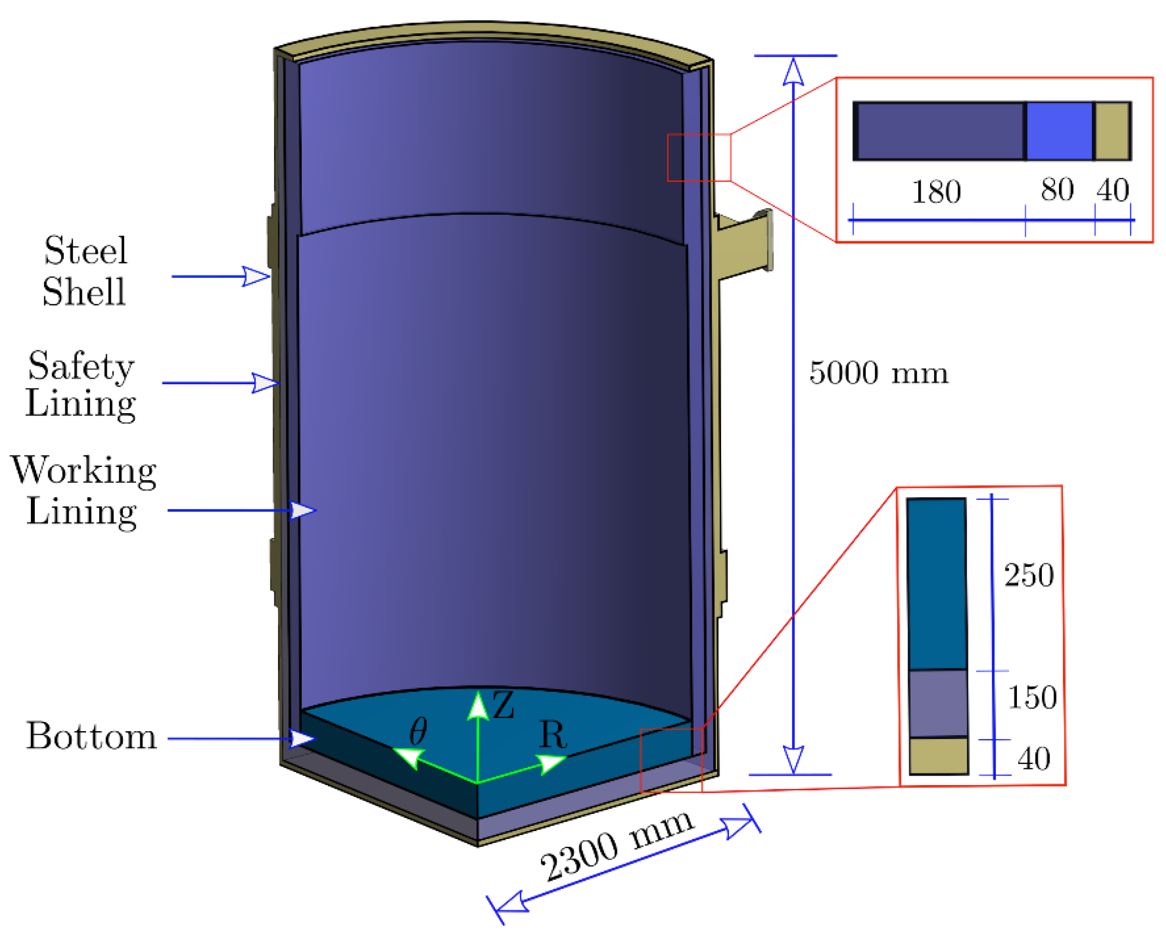
Refractories are the best candidate materials for steel ladle application due to their low thermal conductivity and thermal, chemical, and mechanical stability at high temperatures. To meet the mechanical, thermal, and operational requirements, different refractory layers are used for the construction of the ladle. Each layer has a specific purpose and has unique thermophysical and mechanical properties. The different layers include a working lining, safety lining (also called permanent lining), and steel shell (see Figure 1). The working lining is made of mortarless refractory masonry. The safety lining is composed of two layers: A dense refractory masonry with a mortar joint layer with low thermal conductivity, and a porous layer with lower thermal conductivity. The mechanical and thermophysical properties of each layer are reported in Table 1, where ρ is the density, Cp is the specific heat, k is the thermal conductivity, Y is Young’s modulus, and CTE is the coefficient of thermal expansion.
A typical industrial-scale steel ladle has complex geometry and is composed of refractory linings, steel construction components, valves, purging plugs, a lifting point, etc. In order to reduce the computation time and, as the main aim of the present work is to analyze the thermomechanical behavior of the refractory linings, some detailed features such as valves, nozzles, and purging plugs have been neglected. In addition, due to symmetry, one quarter of the steel ladle has been considered. The simplified physical model of the studied steel ladle is presented in Figure 1. The height and diameter of the ladle are and , respectively. The thickness of each layer is given in and reported in Figure 1.
2.2. Process Description
In the steel industry, steel ladles are used to transport liquid steel from electric arc furnaces or converters to continuous casting machines. In addition, they are used as refining units. While holding liquid steel, other processes occur in parallel such as degassing and alloying. During this process, the ladle is exposed to different thermal and mechanical operating conditions. A typical thermal cycle of steel ladle refractory linings includes: Step 1, preheating the working lining using natural gas burner (to around 1400 ); step 2, slight temperature decrease due to thermal losses while moving from the preheating device to the converter and waiting for liquid steel tapping; step 3, sudden temperature increase due to tapping of liquid steel into the ladle; step 4, gradual temperature drop due to teeming liquid steel out of the ladle, thermal losses during linings check and, if required, linings repair. Further details on thermal modelling and the boundary conditions of each step are given below.
2.3. Thermal and Mechanical Modelling
During the previously described thermal cycle, the temperature distribution of the ladle varies with time and can be obtained by solving the transient form of energy equation given by [15]
where , , , and T are the density, specific heat, thermal conductivity, and temperature, respectively. Before preheating, the initial temperature () of all material layers of the ladle is assumed to be the same as ambient temperature. Under this assumption, the initial boundary conditions can be expressed in terms of cylindrical coordinates ( as
During the first step, a natural gas burner is used to heat the inner surface of the ladle from ambient temperature to around . The time period for this step is around 6.5 h [8]. The dominant heat transfer mode to the lining surface is radiation with only conduction occurring within the thickness of the different layers. Modelling radiative heat transfer between the burner and lining surface requires solving the full Navier–Stokes equations and energy conservation equations that govern the combustion process. This necessitates long computation time and lies outside the scope of the present work. A simple approach that can reasonably simulate the transient thermal response of the ladle during preheating is to consider convective heat transfer between a heat transfer fluid (HTF) and lining surface. The temperature of the HTF () is assumed to be . The convective heat flux on the internal surfaces ( of the ladle can be expressed as
where is the convective heat transfer coefficient during step 1 and is the outward normal to the surface. The radiative and convective thermal losses () from the outer surfaces of the steel shell to the ambient can be written as
where , , and are the ambient temperature (40 °C), emissivity, Stefan–Boltzmann constant, and steel shell outer surface temperature, respectively. This boundary condition has been applied to the external surfaces during the whole steps of the thermal cycle of the ladle.
During step 2, the steel ladle is moved from the heating device to the converter or electric arc furnace and waits to receive the liquid steel. The duration of this step may reach . During this period, the inner and outer surfaces of the ladle exchange heat with the environment by convection and radiation mechanisms. Heat losses of the external surface are expressed by Equation (4), whereas heat losses from the internal surfaces () are written as
with , , and denoting the heat transfer coefficient during step 2, internal surfaces temperature, and environmental temperature (), respectively.
After step 2, liquid steel (with ) is poured inside the steel ladle, leading to a sudden increase in lining temperature (thermal shock). During this step, other processes may occur in parallel (degassing, alloying, etc.), and the total duration of this step is assumed to be . During this period, heat is transferred from the liquid steel to the linings mainly by convection [6]. The convective heat flux on the internal surfaces () can be expressed as
Regarding the last step of the thermal cycle (step 4), liquid steel is drained out of the ladle. The temperatures of the ladle’s internal and external surface decrease gradually due to thermal losses to the ambient. The heat losses during this step are considered similar to those of step 2. It should be noted that the heating and cooling rates during the four steps of the thermal cycle are not constant, as, according to Equations (3), (5) and (6), they are functions of the temperature of the internal surfaces. For example, in the beginning of the first preheating (1st step of 1st thermal cycle), the heating rate is very high as compared to the heating rate at the end of the same step.
The thermal model for steel ladle shown in Figure 1 has been developed using Abaqus software. Then, weak thermomechanical coupling is used. The computed temperature distributions have been used as a thermal load for thermomechanical models. Symmetry boundary conditions have been applied to the symmetric planes of the physical model. The vertical displacement of the bottom of the ladle is assumed to be fixed in the vertical direction (z-direction in Figure 1). The weight and hydrostatic pressure of liquid steel were neglected as their impact on resulting stresses is very small (around 1 MPa) as compared to the impact of the thermal expansion of the bricks (several hundred MPa). The working lining (mortarless refractory masonry) has been replaced by a homogenized equivalent material model that considers joint closure and reopening due to temperature change. Further details about the homogenized equivalent material model and joint closure and reopening criteria are given in Section 3.
3. Mechanical Homogenization of Mortarless Masonry Structure
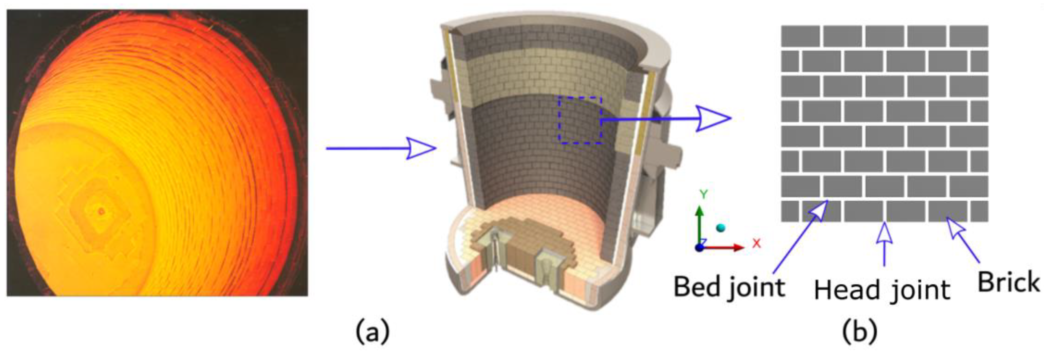
In the present work, the dry-stack refractory masonry structure shown in Figure 2 has been studied. Refractory masonry blocks with length (), height (), and width () are periodically arranged in a running bond texture. Joints with thickness (g << , , ) separate the blocks from each other. These joints are present due to the surface roughness of the blocks and surface shape defaults. Two categories of joints are defined based on their orientation: Bed joints with thickness (in the horizontal direction) and head joints with thickness (in the vertical direction). Under thermal or mechanical loading/unloading, these joints can close and reopen, leading to a change in the overall thermomechanical response of the refractory masonry structure. The influence of the closure and reopening of joints on the mechanical behavior should be taken into account when developing accurate numerical models for the analysis and design of dry-stack masonry structures.
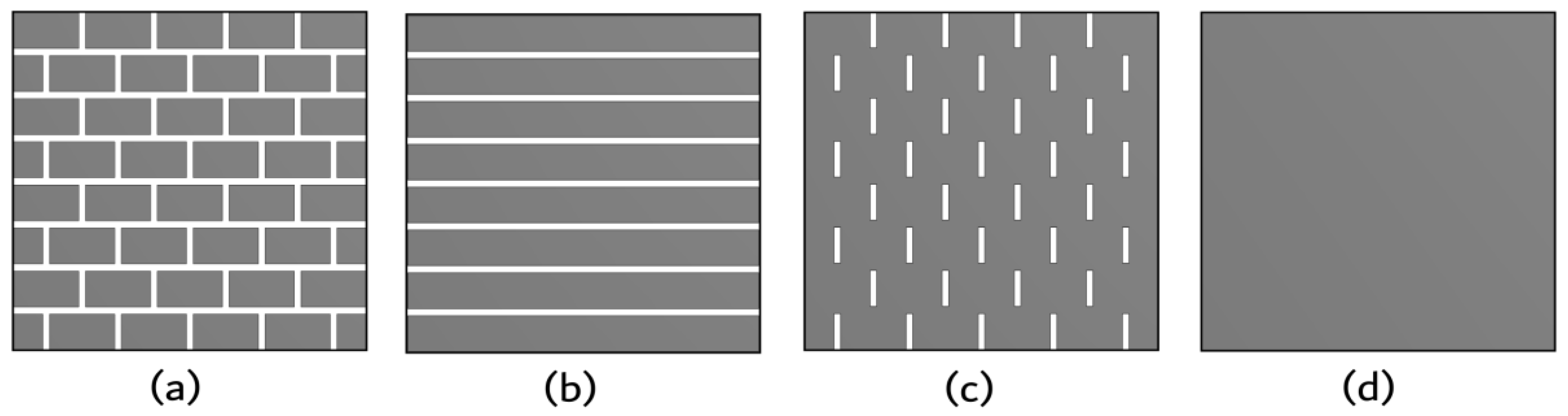
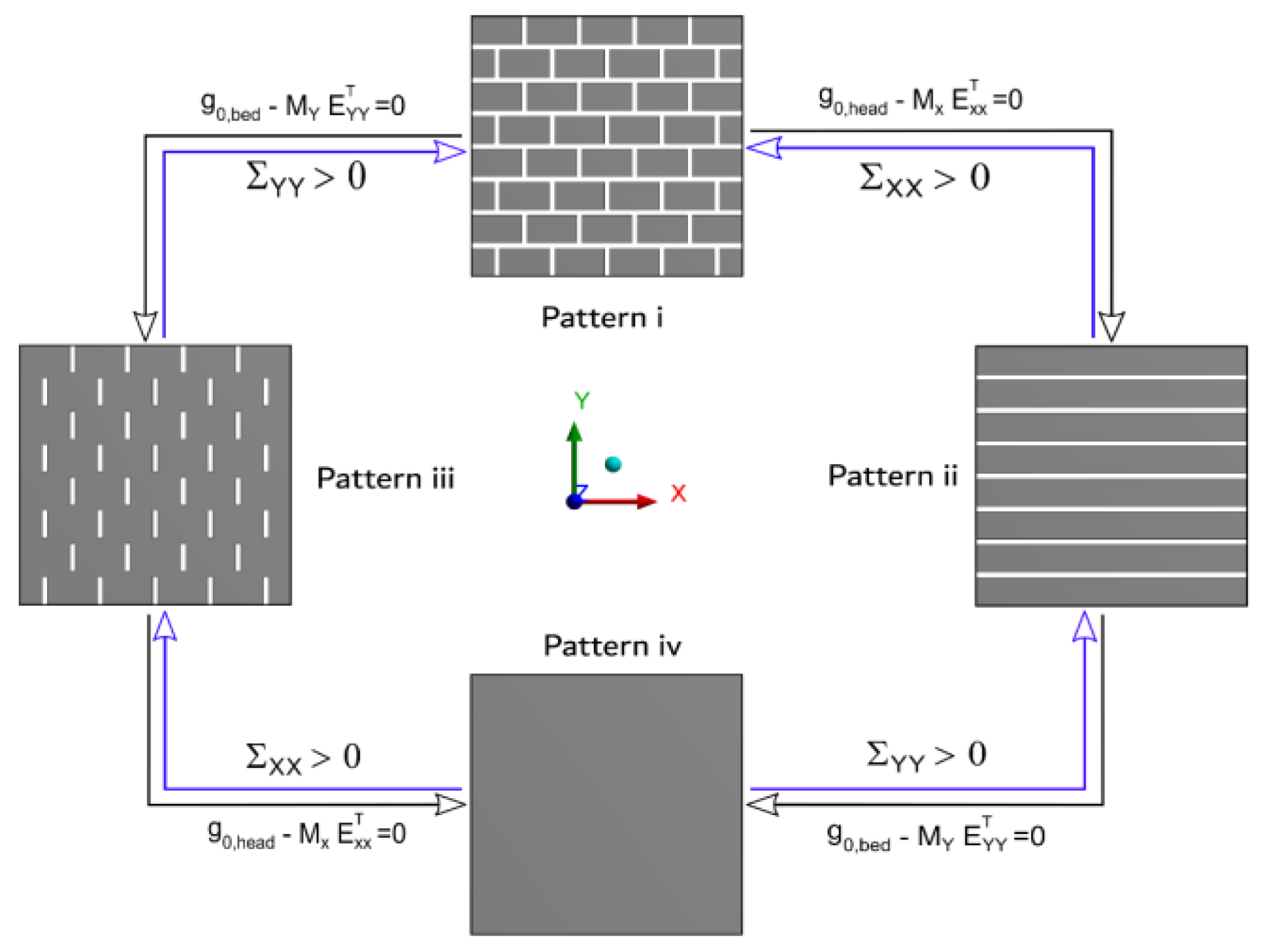
In order to study the influence of the closure and reopening of joints on the overall mechanical behavior of dry-stack masonry structures, four possible joint patterns have been defined (see Figure 3). Each joint pattern is associated with a specific state of bed and head joints (open or closed). The four joint patterns are defined as follows [4]:
- Pattern i: Bed and head joints are open.
- Pattern ii: Bed joints are open, and head joints are closed.
- Pattern iii: Bed joints are closed, and head joints are open.
- Pattern iv: Bed and head joints are closed.
Each joint pattern represents a different periodic masonry structure with different equivalent elastic behavior. Further details on the determination of the equivalent elastic properties of each joint pattern are given in Section 3.1. In addition, criteria of the closure, reopening, and transition of joints from one joint pattern to another are described in Section 3.2.
3.1. Equivalent Mechanical Behavior of Each Joint Pattern
3.1.1. Joint Pattern iv
As previously stated, in the case of joint pattern iv, both bed and head joints are closed (see Figure 3) and, therefore, the macroscopic elastic behavior of the dry-stack masonry structure is similar to that of the constitutive material of the bricks. At high temperature, the constitutive material of the bricks is assumed to undergo small deformations and exhibit isotropic linear elasticity. Under these assumptions, the total strain tensor can be decomposed into elastic and thermal strain tensors according to
Here, , and are the total, elastic, and thermal strains second rank tensor, respectively (in the whole paper, the number of over bars above the symbol indicates the rank of the tensor). The linear elastic strain can be determined using Hooke’s law as
with and denoting Young’s modulus and Poisson’s ratio of the constitutive material. and are the second-order stress tensor and second-order identity tensor, respectively.
3.1.2. Joint Pattern iii
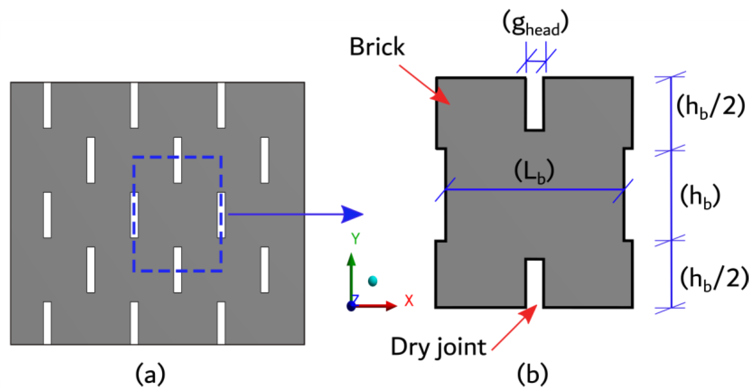
In the case of joint pattern iii, bed joints are closed, whereas head joints are open (see Figure 3). The presence of open joints leads to a decrease in the effective stiffness of the masonry structures [16]. As a result, the macroscopic elastic behavior of joint pattern iii is different from that of the constitutive material of the bricks and can be determined using the finite element-based homogenization technique. To carry out mechanical homogenization of the periodic structures (as joint pattern iii), a periodic representative volume element (RVE) with volume has been selected, as illustrated in Figure 4. Then, 3D finite element simulations have been carried out on the RVE to characterize its homogenized mechanical response and determine the effective mechanical parameters. The constitutive material has been assumed to exhibit an isotropic linear elasticity and obey the constitutive equations given in Section 3.1.1. Periodic boundary conditions have been used to account for the periodicity of the structure and ensure that the deformed external surfaces of the RVE are still periodic [17].
Several finite element simulations of uniaxial tension along the x-, y-, and z-directions, as well as simple shear in the xy, xz, and yz planes, have been performed. From the simulated combination of uniaxial tensile and simple shear tests, the effective elastic stiffness fourth-order tensor () of joint pattern iii has been calculated using Hooke’s law for linear orthotropic elastic materials according to [18]:
with and being the second-order macroscopic stress and the macroscopic elastic strain tensors, respectively. The homogenized or macroscopic stress can be derived by integrating the local stress () over the volume of the unit cell () according to Hill’s definition as follows [19]:
The macroscopic strain has been calculated by dividing the average change in displacement on the corners of the RVE by the initial dimensions of the RVE [20]. From the calculated non-zero components of the elastic stiffness matrix , the effective Young’s modulus (Y), Poisson’s ratio (ν), and shear modulus (G) have been determined.
3.1.3. Joint Pattern i
As mentioned before, in the case of joint pattern i, both bed and head joints are open. One can notice that the mortarless masonry structure is completely disconnected, and between the bricks, there are small gaps (see Figure 3). For computing the effective mechanical properties, one cannot apply the finite element-based periodic homogenization technique described previously, because the homogenization problem of the cell is not clearly known. However, instead, the effective mechanical properties can be assigned directly [4,5]. Due to the presence of open joints, the macroscopic stiffness of the masonry structure in the x- and y-directions is very small. The effective Young’s modulus of the masonry is zero in the x- and y-directions (see the coordinate system in Figure 4). However, the effective Young’s modulus in the z-direction is the same as that of the brick as there are no joints in this direction. Values of the macroscopic elastic constants are reported in Table 2, where , , and are Young’s modulus, Poisson’s ratio, and the shear modulus of the constitutive material. To facilitate the numerical computations and avoid numerical singularities, a very small value has been assigned to ,, , , , and instead of zero.
3.1.4. Joint Pattern ii
Regarding joint pattern ii, bed joints are open, whereas head joints are closed (see Figure 3). The mortarless masonry structure is composed of an array of separated courses (in y-direction) of bricks. Therefore, the structure has no stiffness in the y-direction, while it has stiffness in the x-direction [4,5]. Similar to joint pattern i, one can define the macroscopic elastic parameters directly. As bed joints are open, the material stiffness in the y-direction is very small and is zero. However, as head joints are closed, has the same value as the bricks. In addition, Young’s modulus in the z-direction has the same value as the brick as there are no joints in this direction. The effective material parameters for the four joint patterns are listed in Table 2.
3.2. Joint Closure and Reopening Criteria
As discussed before, for each joint pattern, the equivalent constitutive model has different elastic behaviors. During operation, the masonry structure is subjected to cyclic thermal heating/cooling. As a result, bed and/or head joints may close (or reopen). Therefore, the structure may change from one pattern to another, leading to a change in the homogenized elastic behavior. This change has been considered by using a suitable joint closure/reopening and pattern transition criterion.
Before loading, the initial joint pattern is usually pattern 1 (bed and head joints are open). Under compression, the bed and/or head joint thickness decrease gradually from the initial value (, from 0.1 to 0.2 mm) until reaching zero, and the structure will change to state ii (if head joints close), iii (if bed joints close), or iv (if both bed and head joints close). Bed or head joints are considered to be open or closed based on the instantaneous thickness of joint () according to
As the equivalent material properties are piecewise constant, the displacement increment at every point in the masonry linearly depends on the increment in macroscopic quantities. As a result, one can define the instantaneous thickness of the bed and head joints in terms of macroscopic strains according to [4,5]
Here, and are the instantaneous thickness of the head and bed joint, respectively. and are the initial thickness of head and bed joints, respectively. and are parameters with the same meaning of localization tensor and they depend on the dimensions of the brick ( and ). and are the macroscopic total strains (elastic and thermal strains) in the x- and y-directions, respectively.
Regarding the joint reopening criterion, bed and head joints can reopen if the stress normal to the surface of the joint (bed or head) is higher than zero. This means that a bed joint can reopen if and a head joint can reopen if . As homogeneous stresses are linearly dependent on local stresses (see Equation (10)), one can rewrite the joint reopening criterion in terms of macroscopic stresses using the localization tensor . and can be written in terms of macroscopic strains and non-zero components of the macroscopic stiffness matrix as follows [5]:
Here, denotes the non-zero components of the elastic stiffness tensor determined in previous sections. The transition criteria between pattern i and ii, pattern ii and iii, pattern ii and iv, pattern iii and pattern iv, and vice versa are illustrated in Figure 5.
4. Results and Discussion
4.1. Validation of the Developed Homogenized Material Model
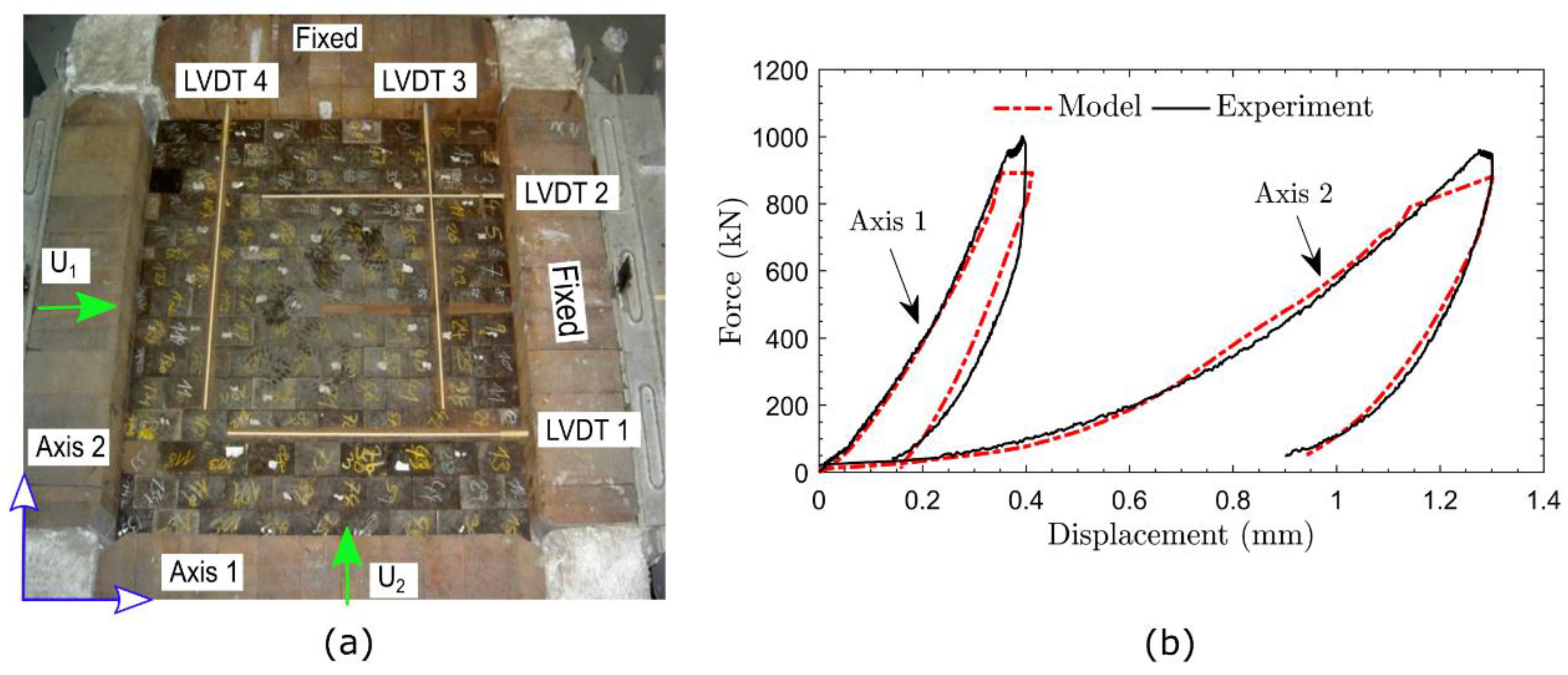
In order to validate the developed homogenized equivalent material model, comparisons between experimental and numerical results of the mortarless masonry structure subjected to biaxial compression have been carried out. As can be seen in Figure 6a, the biaxial compression test setup is composed of dry-stack masonry surrounded by four ceramic plates. Two of them are fixed, whereas the others can move and are connected to hydraulic pistons. Four linear variable differential transformers (LVDTs) are used to measure the displacement in directions one and two or “along bed joints and along head joints direction.” The biaxial compression test is as follows: First, a preload is applied in two directions at the same time and is stopped first in the direction for which the LVDTs detect a displacement; it then stops in the second direction when the LVDTs detect a displacement in the corresponding direction. Finally, loads in both directions have been applied at the same time. Displacements, as well as reaction forces, of the moving ceramic plates were recorded. The size of the mortarless masonry is and the dimensions of the refractory brick are . Bricks are periodically arranged in a running bond texture and the masonry comprises 14 courses. The constitutive material of the bricks is magnesia-chrome with Young’s modulus of , and Poisson’s ratio of .
The homogenized material model presented in Section 3 has been implemented into Abaqus software using the user material subroutine (UMAT) and has then been used to simulate the biaxial compression test. The four ceramic plates, as well as the support device, have been modeled as rigid plates. Two of them are fixed while displacement boundary conditions have been applied to the other two. Friction between the bricks and the rigid plates and between the bricks and the support device has been considered.
Figure 6b shows a comparison between experimental and numerical results. As can be seen from the figure, both numerical and experimental results are in good agreement. The overall behavior of the masonry is orthotropic and nonlinear due to the gradual closure/reopening of the joints and changing from one joint pattern to another. The reaction forces, in the two directions, increase with the increase in the applied displacement due to the gradual closure of the joints and the increase in material stiffness with joints closure. The displacement in direction 2 is higher than the displacement in direction 1 as the number of joints in direction 2 is higher than that in direction 1 (13 bed joints in direction 2 and 8 head joints in direction 1). After unloading, the masonry structure will not return to the initial configuration and there will always be permanent deformation in both directions. This can be attributed to the final joint thickness in both directions being less than that of the initial one.
4.2. Temperature Distribution
The previous results have shown the capability of the presented homogenized material model to describe the homogenized orthotropic nonlinear elastic behavior of mortarless masonry structures. Thus, it has been used to analyze the transient thermomechanical response of the mortarless refractory masonry structure used in steel ladles. The working lining (mortarless masonry structure) of the steel ladle model shown in Figure 1 and described in Section 2 has been replaced by the developed equivalent material model. Three full production cycles have been modelled to investigate the impact of cyclic temperature change and joint thickness on the thermomechanical behavior of a steel ladle.
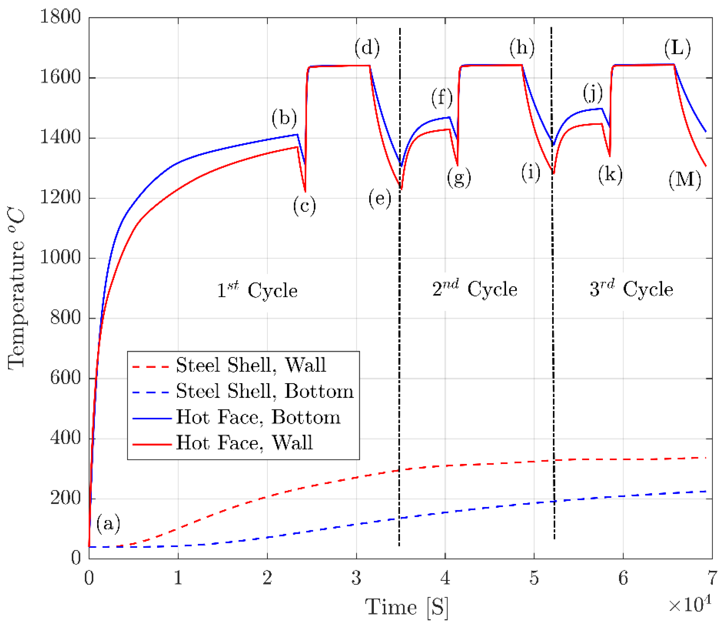
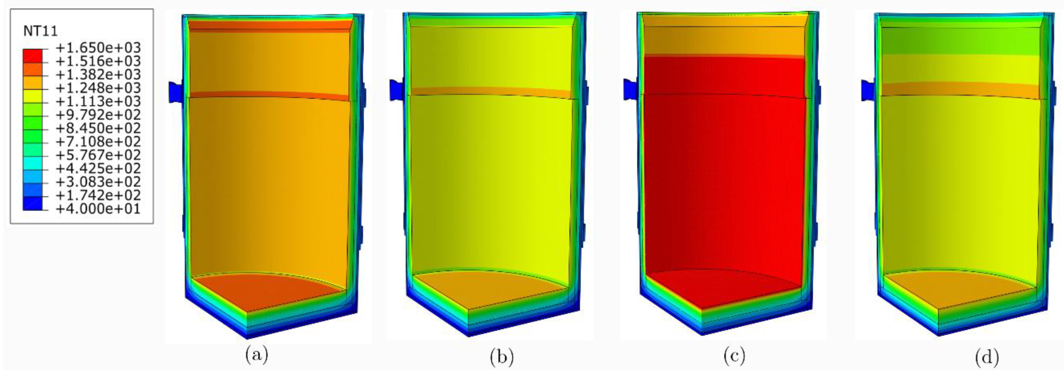
Time variations of the temperature of the working lining hot face (surface in contact with liquid steel) and steel shell outer surface (bottom and wall) during the first three complete production cycles are shown in Figure 7. Temperature distributions at the end of step 1, the end of step 2, the beginning of step 3, and the end of step 4 of the first thermal cycle are presented in Figure 8 (see Table 3 for full description of the three simulated thermal cycles). As explained earlier, during the first step (a to b), heat is transferred by the forced convection mechanism from a heat transfer fluid at to the working lining (initial temperature is about ). As a result, the temperature of the working lining increases gradually from room temperature to around . Then, the steel ladle is transported from the heating device to the converter or electric arc furnace while losing heat to the environment by convection and radiation mechanisms (b to c). This leads to a drop in the temperature to around . After that (c to d), liquid steel at around is tapped into the ladle, resulting in a sudden increase in the temperature. At the end of the thermal cycle (d to e), the working lining temperature decreases gradually. The observed decrease in temperature can be attributed to the teeming of liquid steel and heat losses (by convection and radiation mechanisms) from external and internal surfaces of the ladle to the ambient.
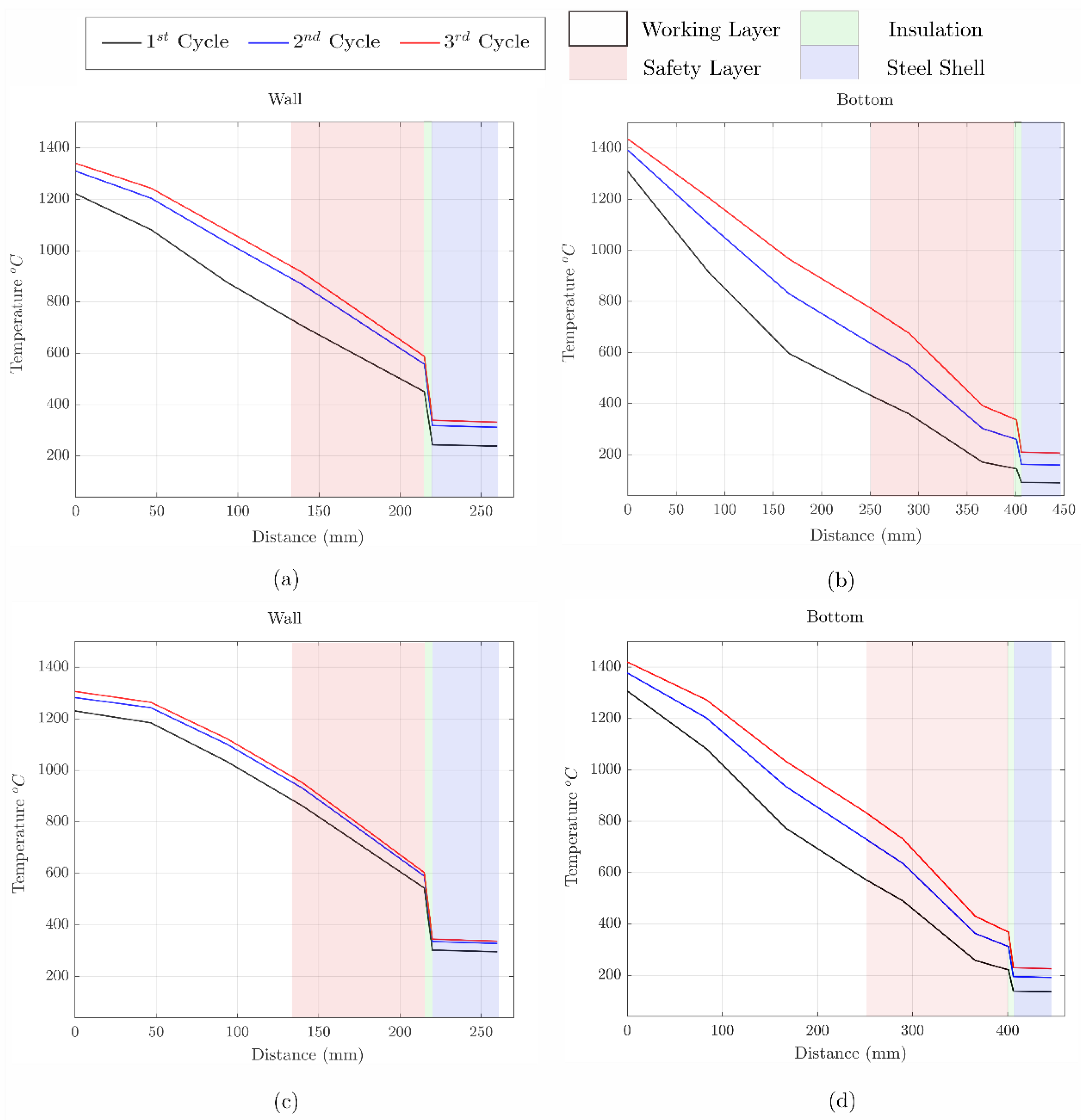
Comparisons between temperature gradient through the thickness of the steel ladle’s wall and bottom at the end of step 2 and end of step 4 of the first three full steel ladle’s thermal cycle are shown in Figure 9. For the second and third thermal cycles, after preheating, the temperature of the working lining is slightly higher when compared to the temperature at the end of the first preheating (points f and j as compared to point b in Figure 7). Similarly, the working lining temperature at the end of step 2 (points g and k in Figure 7) and 4 (points i and m in Figure 7) of production cycle 2 and 3 is slightly higher than that of the first thermal cycle (point c at end of step 2 and point e at end of step 4 in Figure 7). This behavior is caused by the overall temperature increase of the ladle after the first preheating cycle (see Figure 9). It should be mentioned that during the first step of the three simulated production cycles, the inner surface temperature of the bottom is slightly higher than that of the wall. In addition, the steel shell bottom outer surface temperature is lower compared to that of the steel shell wall. This can be explained by the fact that the thickness of the working and safety lining at the bottom is higher than that at the wall.
4.3. Stress Fields
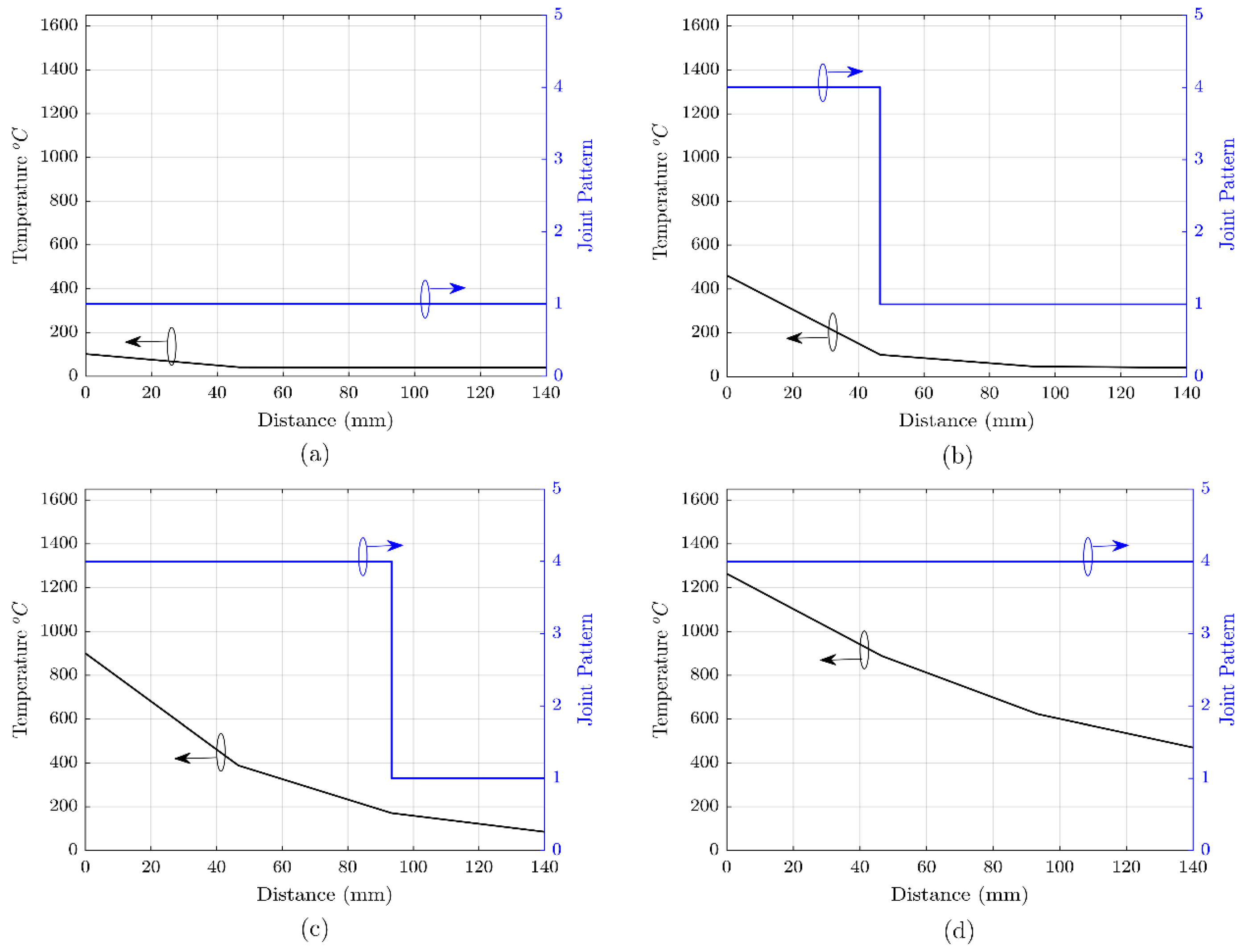
The gradual closure and reopening of the joints due to temperature fluctuations during the three thermal cycles are shown in Figure 10. Initially (at time = 0 s), bed and head joints are open and, therefore, the working lining (bottom and wall) is in pattern 1. With the increase in temperature, joints close gradually due to the thermal expansion of the bricks. It has been noticed that joints at the working lining hot surface (internal surface of the ladle) usually close before joints at the cold surface (surface in contact with the permanent lining) (see Figure 11). At almost 700 s, all joints in the hot face are closed and remain closed until the end of step 1. At the end of step 2, some joints at the outer top surface of the slag zone (see Figure 10f) reopen. This can be attributed to thermal losses, the temperature drop of this region and, therefore, the change in stress from compression to tension. These open joints close again owing to liquid steel pouring inside the ladle and the sudden increase in temperature. As the temperature drop during step 4 is higher than that during step 2, one can notice that at the end of step 4, more joints are open as compared to the number of open joints at the end of step 2. Therefore, waiting time (after preheating and before liquid steel tapping) is an important issue to consider when defining the time period of each step of the ladle thermal cycle. Long waiting time leads to high energy losses and may result in the opening of the joints at the wall and the bottom of the steel ladle just before tapping liquid steel in the ladle. Further analysis to investigate the impact of preheating temperature, joint thickness, and waiting time on joint reopening is planned to be carried out in the future.
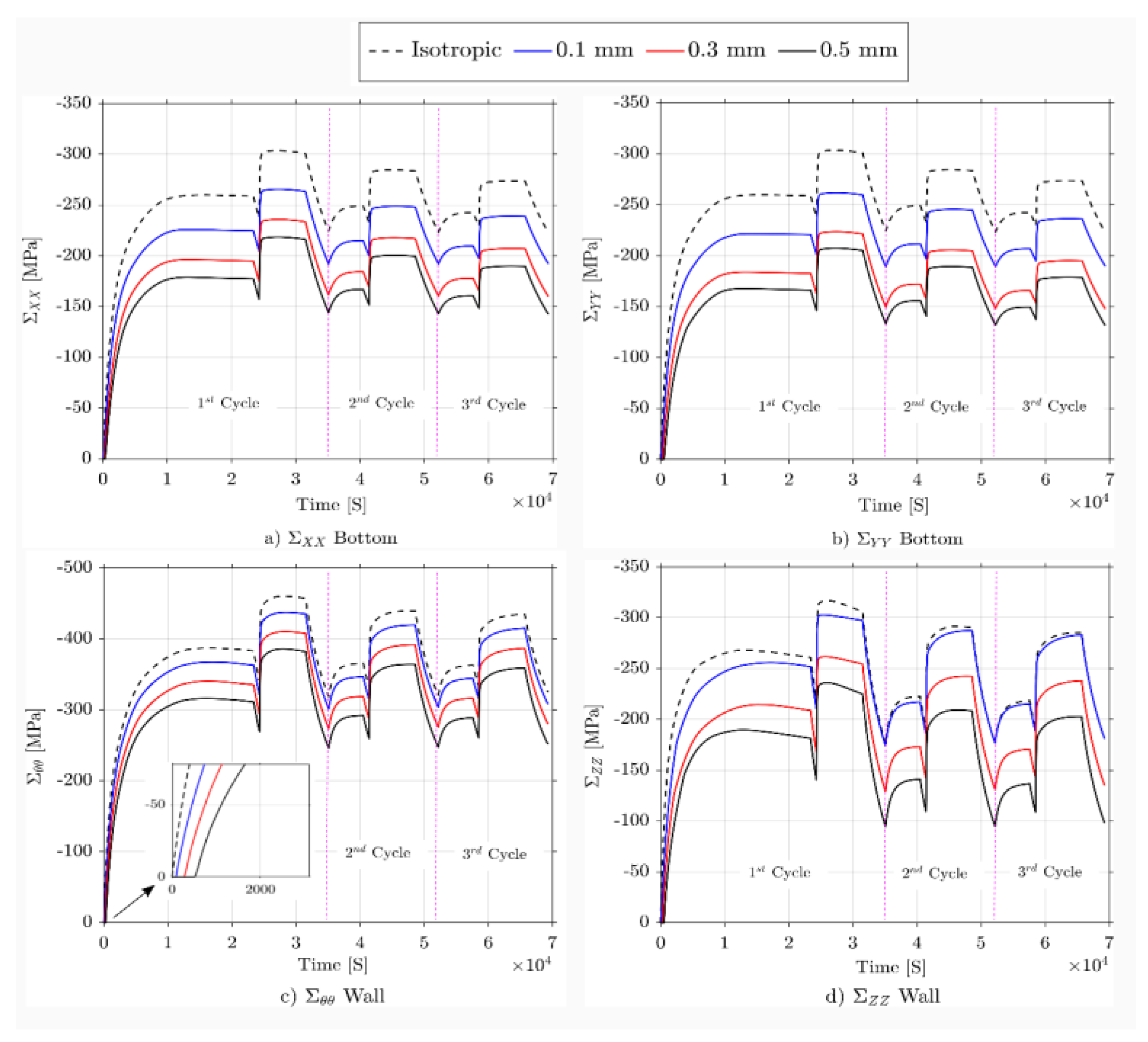
Time variations of the thermal stresses in the hot face of the bottom (center, ) and wall (middle, ) of the working lining for different values of bed and head joint thickness (, and ), as well as isotropic representation of mortarless masonry (i.e., presence of joints is neglected and properties of the structure are assumed to be the same as those of the bricks), during the first three heating cycles are shown in Figure 12. The brick length and height are taken as and , respectively, and the depth of the bricks is given in Figure 1. In general, it has been observed that the resulting thermal stresses increase with the increase in temperature, decrease with the increase in joint thickness, and their trends are similar to those of the temperature during the four steps of the ladle thermal cycle. In addition, the isotropic assumption of mortarless masonry leads to an overestimation of resulting thermal stresses.
During the first step, thermal stresses increase with the increase in temperature and thermal expansion of the bricks. Then (during step 2), they decrease slightly due to the temperature decrease and contraction of the bricks. The maximum value of thermal stresses is reached when liquid steel is tapped in the steel ladle. This is because of the sudden increase in temperature. During step 4, they decrease again with the decrease in temperature. Finally, this trend is repeated. However, for the second and third thermal cycles, resulting thermal stresses are lower as compared to those of the first thermal cycle. This can be attributed to the fact that, at the beginning of the second and third thermal cycles, the initial temperature of the steel ladle is much higher compared to that of the first heat cycling. Therefore, for second and third thermal cycles, temperature gradient histories are low compared to those of the first thermal cycle. Moreover, one can notice that the hot face is under high compressive stresses. This result may be explained by the fact that the temperature of the hot face is higher than the temperature of the other layers and tends to expand faster than the safety, insulation layers, and the steel shell.
Increasing joint thickness leads to a decrease in the resulting thermal stresses in the bottom and the wall of the working lining, as well as the steel shell. Increasing joint thickness allows the bricks to expand freely (until closure of joints), resulting in lower values of thermal stresses. After closure of joints, thermal stresses increase at a higher rate. This phenomenon is shown in Figure 10c. In the first 500 s, as joints are closing during this period, the values of the resulting thermal stresses are very small.
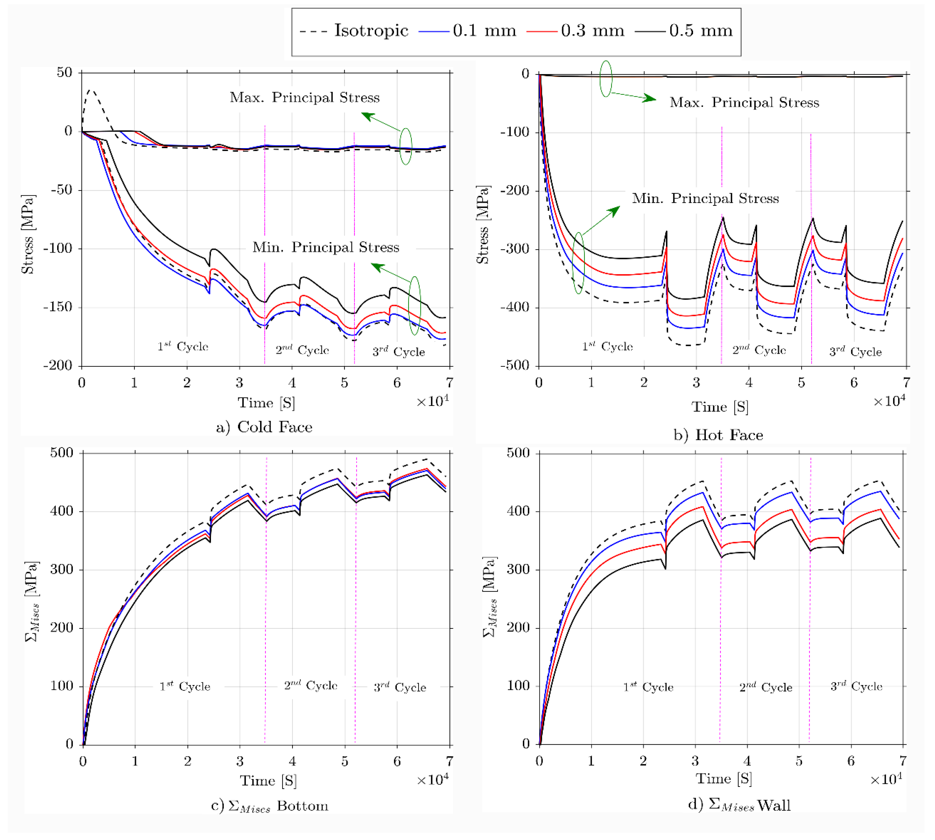
Time variations of the maximum and minimum principal stresses in the hot face and cold face of the working lining, as well as Von Mises stresses in the steel shell (bottom and wall), are depicted in Figure 13. Overall, increasing joint thickness leads to a decrease in the maximum and minimum principal stresses in the working lining (hot and cold face) and Von Mises stresses in the steel shell. Values of minimum principal stresses in the cold face are less than those of the hot face, because, as discussed earlier, the hot face temperature is higher as compared to the cold face temperature. At the first 10,000 s, values of maximum principal stresses in the cold face are positive and, as discussed earlier, joints are open (i.e., macroscopic material stiffness in - and z-directions is very small). Therefore, using the homogenization technique, lower values of maximum principal stresses are predicted (less than 2 MPa) as compared to the values (around 40 MPa) predicted using the isotropic representation of masonry (i.e., presence of joints neglected and material stiffness in - and z- directions are similar to those of the bricks).
5. Conclusions and Perspective
In the present work, three-dimensional coupled sequential thermomechanical analysis of a steel ladle has been carried out. The working lining and the bottom of the ladle have been replaced by an equivalent material model that takes into account the closure and reopening of joints due to cyclic thermal or mechanical loading/unloading. The temperature distribution of the steel ladle has been computed and used as a thermal load for the thermomechanical analysis. The thermomechanical model enables the visualization of the gradual closure and reopening of joints during the complete thermal cycle of the ladle. The impact of joint thickness on the resulting thermal stresses has been studied. The following conclusions can be drawn:
- With the increase in temperature, dry joints close gradually due to the thermal expansion of the bricks. Joints at the working lining hot surface close faster than joints at the cold surface.
- The temperature drop during the waiting time results in the opening of some joints at the outer top surface of the slag zone. Moreover, waiting time is an important issue to consider when defining the time period of each step of the ladle thermal cycle. Long waiting time leads to high energy losses and may result in the opening of joints at the wall and the bottom of the steel ladle just before tapping liquid steel in the ladle.
- Resulting thermal stresses in the hot face increase with the increase in temperature, and their trends are similar to those of the temperature during the four steps of the thermal ladle heating cycle. However, during the second and third thermal cycle, values of resulting thermal stresses are low compared to those of the first thermal cycle, as the maximum stress is proportional to the difference between the local maximum temperature and the average temperature in the thickness. Thus, after the second and third cycles, the average temperature is higher and the stress then decreases.
- The working lining hot face is under high compressive stresses; on the other hand, the cold face is under tensile stresses when joints are open during the first 10,000 s of step 1 of the first thermal cycle (1st preheating) and heat loss steps (steps 2 and 4 of the thermal cycle).
- Increasing joint thickness leads to a decrease in the resulting thermal stresses in the bottom and the wall of the working lining, as well as in the steel shell.
In perspective, this study could be exploited as the first step in nonlinear multi-scale thermomechanical analysis of refractory masonry structures. Further parametric studies to investigate the maximum possible joint thickness, wherein preheating will not allow enough closure to contain liquid steel, are planned to be carried out in the future. In addition, further developments of the equivalent material model to consider the creep of the mortarless refractory masonry structure will allow better prediction of thermal stress levels, and the design and optimization of thermally and mechanically efficient steel ladles. Work on this line is ongoing at LaMé laboratory, University of Orléans.
Author Contributions
Conceptualization, M.A., A.G. and T.S.; methodology, M.A., A.G. and T.S.; software, M.A. and T.S.; validation, M.A.; formal analysis, M.A.; investigation, M.A.; resources, M.A.; writing—original draft preparation, M.A.; writing—review and editing, A.G., T.S. and E.B.; visualization, M.A.; supervision, T.S., A.G. and E.B.; project administration, A.G.; funding acquisition, A.G. and E.B. All authors have read and agreed to the published version of the manuscript.
Funding
This work was supported by the funding scheme of the European Commission, Marie Skłodowska Curie Actions Innovative Training Networks in the frame of the project ATHOR - Advanced Thermomechanical mOdelling of Refractory linings 764987 Grant.
Acknowledgments
The authors are grateful to the Centre de Calcul Scientifique en région Centre Val de Loire (France) for the computation time and technical support.
Conflicts of Interest
The authors declare no conflict of interest.
References
- Blond, E.; Schmitt, N.; Hild, F.; Blumenfeld, P.; Poirier, J. Effect of Slag Impregnation on Thermal Degradations in Refractories. J. Am. Ceram. Soc. 2007, 90, 154–162. [Google Scholar] [CrossRef] [Green Version]
- Andreev, K.; Sinnema, S.; Rekik, A.; Allaoui, S.; Blond, E.; Gasser, A. Compressive behaviour of dry joints in refractory ceramic masonry. Constr. Build. Mater. 2012, 34, 402–408. [Google Scholar] [CrossRef] [Green Version]
- Allaoui, S.; Rekik, A.; Gasser, A.; Blond, E.; Andreev, K. Digital Image Correlation measurements of mortarless joint closure in refractory masonries. Constr. Build. Mater. 2018, 162, 334–344. [Google Scholar] [CrossRef]
- Nguyen, T.M.H.; Blond, E.; Gasser, A.; Prietl, T. Mechanical homogenisation of masonry wall without mortar. Eur. J. Mech. A Solids 2009, 28, 535–544. [Google Scholar] [CrossRef]
- Ali, M.; Sayet, T.; Gasser, A.; Blond, E. Thermomechanical Modelling of Refractory Mortarless Masonry Wall Subjected to Biaxial Compression. In Proceedings of the Unified International Technical Conference of Refractories, Yokohama, Japan, 13–16 October 2019. [Google Scholar]
- Xia, J.L.; Ahokainen, T. Transient flow and heat transfer in a steelmaking ladle during the holding period. Metall. Mater. Trans. B 2001, 32, 733–741. [Google Scholar] [CrossRef]
- Glaser, B.; Görnerup, M.; Sichen, D. Fluid Flow and Heat Transfer in the Ladle during Teeming. Steel Res. Int. 2011, 82, 827–835. [Google Scholar] [CrossRef]
- Santos, M.F.; Moreira, M.H.; Campos, M.G.G.; Pelissari, P.I.B.G.B.; Angélico, R.A.; Sako, E.Y.; Sinnema, S.; Pandolfelli, V.C. Enhanced numerical tool to evaluate steel ladle thermal losses. Ceram. Int. 2018, 44, 12831–12840. [Google Scholar] [CrossRef]
- Yilmaz, S. Thermomechanical Modelling for Refractory Lining of a Steel Ladle Lifted by Crane. Steel Res. Int. 2003, 74, 485–490. [Google Scholar] [CrossRef]
- Hou, A.; Jin, S.; Harmuth, H.; Gruber, D. A Method for Steel Ladle Lining Optimization Applying Thermomechanical Modeling and Taguchi Approaches. JOM 2018, 70, 2449–2456. [Google Scholar] [CrossRef]
- Gasser, A.; Chen, L.; Genty, F.; Daniel, J.L.; Blond, E.; Andreev, K.; Sinnema, S. Influence of different masonry designs of bottom linings. In Proceedings of the Unified International Technical Conference of Refractories, Victoria, BC, Canada, 10–13 September 2013. [Google Scholar]
- Shakhtin, D.M.; Pechenezhskii, V.I.; Karaulov, A.G.; Kvasman, N.M.; Kravchenko, V.P.; Kabakova, I.I.; Ustichenko, V.A.; Kalita, G.E.; Shcherbenko, G.N.; Yakobchuk, L.M. Thermal conductivity of corundum, high-alumina, magnesia, zirconium, and chromate refractories in the 400–1800 °C range. Refractories 1982, 23, 223–227. [Google Scholar] [CrossRef]
- Nemets, I.I.; Nestertsov, A.I.; Zagoskin, V.T.; Vysotskii, D.A.; Stavrovskii, G.I.; Chekhovskoi, V.Y. The thermal conductivity of periclase and periclase—Spinel refractories. Refractories 1975, 16, 178–180. [Google Scholar] [CrossRef]
- Díaz, L.A.; Torrecillas, R.; Simonin, F.; Fantozzi, G. Room temperature mechanical properties of high alumina refractory castables with spinel, periclase and dolomite additions. J. Eur. Ceram. Soc. 2008, 28, 2853–2858. [Google Scholar] [CrossRef]
- Pletcher, R.H.; Tannehill, J.C.; Anderson, D. Computational Fluid Mechanics and Heat Transfer; CRC Press: Boca Raton, FL, USA, 2012. [Google Scholar]
- Rekik, A.; Nguyen, T.T.N.; Gasser, A. Multi-level modeling of viscoelastic microcracked masonry. Int. J. Solids Struct. 2016, 81, 63–83. [Google Scholar] [CrossRef]
- Xia, Z.; Zhang, Y.; Ellyin, F. A unified periodical boundary conditions for representative volume elements of composites and applications. Int. J. Solids Struct. 2003, 40, 1907–1921. [Google Scholar] [CrossRef]
- Iltchev, A.; Marcadon, V.; Kruch, S.; Forest, S. Computational homogenisation of periodic cellular materials: Application to structural modelling. Int. J. Mech. Sci. 2015, 93, 240–255. [Google Scholar] [CrossRef]
- Hill, R. The essential structure of constitutive laws for metal composites and polycrystals. J. Mech. Phys. Solids 1967, 15, 79–95. [Google Scholar] [CrossRef]
- Michel, J.C.; Moulinec, H.; Suquet, P. Effective properties of composite materials with periodic microstructure: a computational approach. Comput. Methods Appl. Mech. Eng. 1999, 172, 109–143. [Google Scholar] [CrossRef]
Figure 1.
Schematic of a steel ladle showing the different zones and linings.

Figure 2.
Steel ladle lined with dry-stack refractory masonry: (a) Section view and (b) schematic of dry-stack masonry structure.
Figure 2.
Steel ladle lined with dry-stack refractory masonry: (a) Section view and (b) schematic of dry-stack masonry structure.

Figure 3.
Possible joint patterns of mortarless refractory masonry structure: (a) Pattern i, (b) pattern ii, (c) pattern iii, and (d) pattern iv.
Figure 3.
Possible joint patterns of mortarless refractory masonry structure: (a) Pattern i, (b) pattern ii, (c) pattern iii, and (d) pattern iv.

Figure 4.
Schematic of (a) periodic mortarless masonry structure in state 3 and (b) unit cell used in the present study.
Figure 4.
Schematic of (a) periodic mortarless masonry structure in state 3 and (b) unit cell used in the present study.

Figure 5.
Possible joint patterns of mortarless refractory masonry structure and joint closure/reopening criteria.
Figure 5.
Possible joint patterns of mortarless refractory masonry structure and joint closure/reopening criteria.

Figure 6.
(a) Biaxial compression test setup [4] and (b) comparison between experimental and numerical results.
Figure 6.
(a) Biaxial compression test setup [4] and (b) comparison between experimental and numerical results.

Figure 7.
Temperature evolution of inner surface of working lining wall, and bottom and outer surface of steel shell during the first three thermal cycles of steel ladle.
Figure 7.
Temperature evolution of inner surface of working lining wall, and bottom and outer surface of steel shell during the first three thermal cycles of steel ladle.

Figure 8.
Temperature distributions at the (a) end of step 1 (point b in Figure 7), (b) end of step 2 (point c in Figure 7), (c) end of step 3 (point d in Figure 7), and (d) end of step 4 (point e in Figure 7) of the first thermal cycle of the steel ladle.

Figure 9.
Temperature gradient through the thickness of the steel ladle’s wall and bottom at (a,b) end of step 2 and (c,d) end of step 4 of three full ladle’s thermal cycles (see Table 3 for more details about each step of the thermal cycle).
Figure 9.
Temperature gradient through the thickness of the steel ladle’s wall and bottom at (a,b) end of step 2 and (c,d) end of step 4 of three full ladle’s thermal cycles (see Table 3 for more details about each step of the thermal cycle).

Figure 10.
Gradual closure and reopening of joints due to temperature fluctuations during the first heating cycle for joint thickness of 0.1 mm. (a) Time = 0 s (point a in Figure 7), (b) time = 460 s, (c) time = 675 s, (d) time = 1825 s ((b) to (d) correspond to points after point a and before point b in Figure 7), (e) time = 7500 s (point b in Figure 7), (f) time = 24,300 s (point c in Figure 7), (g) time = 24,500 s (point d in Figure 7), (h) time = 33,300 s (point e in Figure 7), and (i) schematic of the four joint patterns.

Figure 11.
Temperature gradient and joint pattern through the thickness of the working lining (height = 2500 mm) for 0.1 mm bed and head joint thickness at (a) time = 50 s, (b) time = 675 s, (c) time = 1825 s, and (d) time = 7500 s.
Figure 11.
Temperature gradient and joint pattern through the thickness of the working lining (height = 2500 mm) for 0.1 mm bed and head joint thickness at (a) time = 50 s, (b) time = 675 s, (c) time = 1825 s, and (d) time = 7500 s.

Figure 12.
(a,b) Time variations of the thermal stresses at the bottom surface and (c,d) wall surface of the working lining for different values of bed and head joint thickness during the first three thermal cycles of the steel ladle.
Figure 12.
(a,b) Time variations of the thermal stresses at the bottom surface and (c,d) wall surface of the working lining for different values of bed and head joint thickness during the first three thermal cycles of the steel ladle.

Figure 13.
Time variations of maximum and minimum principal stresses in the (a) cold face and (b) hot face of the working lining, as well as Von Mises stresses in the steel shell (c) bottom and (d) wall.
Figure 13.
Time variations of maximum and minimum principal stresses in the (a) cold face and (b) hot face of the working lining, as well as Von Mises stresses in the steel shell (c) bottom and (d) wall.


Table 1.
Thermophysical properties of materials used in the present study.
| Lining | Zone | Properties | References | |
|---|---|---|---|---|
| Steel shell | Steel shell | ρ (kg/m3) | 7840 | [8,10] |
| k (W/m.K) | 47.3 at 200 °C 42.3 at 350 °C 37.3 at 500 °C | |||
| Cp (J/kg.K) | 530 at 200 °C | |||
| Y (GPa) | 210 at 20 °C 170 at 400 °C | |||
| CTE ( | 12 | |||
| Safety Lining | Bottom and wall bricks (dense layer) | ρ (kg/m3) | 2660 | [12] |
| k (W/m.K) | 2.6 at 400 °C 2.1 at 800 °C 2 at 1200 °C | |||
| Cp (J/kg.K) | 1144 at 1200 °C | |||
| Y (GPa) | 45 | |||
| CTE ( | 6 | |||
| Bottom and wall insulation (porous layer) | ρ (kg/m3) | 510 | [8,10] | |
| k (W/m.K) | 0.15 at 250 °C 0.25 at 800 °C 0.34 at 1350 °C | |||
| Cp (J/kg.K) | 1047 | |||
| Y (GPa) | 0.3 | |||
| CTE ( | 9 | |||
| Working Lining | Bottom and wall | ρ (kg/m3) | 3210 | [10,13,14] |
| k (W/m.K) | 4.65 at 400 °C 3.49 at 700 °C 4.65 at 1000 °C 5.81 at 1300 °C | |||
| Cp (J/kg.K) | 1090 | |||
| Y (GPa) | 35 at 20 °C 37 at 1000 °C 38 at 1500 °C | |||
| CTE ( | 11 | |||
Table 2.
Effective mechanical properties of the four joint patterns of mortarless refractory masonry structure.
Table 2.
Effective mechanical properties of the four joint patterns of mortarless refractory masonry structure.
| Parameter | Pattern i | Pattern ii | Pattern iii | Pattern iv |
|---|---|---|---|---|
| 0 | 1 | 1 | ||
| 0 | 0 | |||
| 0 | 0 | |||
| 0 | ||||
| 0 | 0 | |||
| 0 | 0 | |||
1 The subscript h denotes brick homogenization, and the subscript b denotes the brick property.
Table 3.
Summary of the three simulated thermal cycles of steel ladle, time period of each step, and corresponding points in Figure 7.
Table 3.
Summary of the three simulated thermal cycles of steel ladle, time period of each step, and corresponding points in Figure 7.
| First Cycle | Second Cycle | Third Cycle | ||||
|---|---|---|---|---|---|---|
| Duration (h) | Corresponding Points | Duration (h) | Corresponding Points | Duration (h) | Corresponding Points | |
| Step 1 | 6.5 | a to b | 1.5 | e to f | 1.5 | i to j |
| Step 2 | 0.25 | b to c | 0.25 | f to g | 0.25 | j to k |
| Step 3 | 2 | c to d | 2 | g to h | 2 | k to L |
| Step 4 | 1 | d to e | 1 | h to i | 1 | L to M |
© 2020 by the authors. Licensee MDPI, Basel, Switzerland. This article is an open access article distributed under the terms and conditions of the Creative Commons Attribution (CC BY) license (http://creativecommons.org/licenses/by/4.0/).
Share and Cite
MDPI and ACS Style
Ali, M.; Sayet, T.; Gasser, A.; Blond, E. Transient Thermo-Mechanical Analysis of Steel Ladle Refractory Linings Using Mechanical Homogenization Approach. Ceramics 2020, 3, 171-189. https://0-doi-org.brum.beds.ac.uk/10.3390/ceramics3020016
AMA Style
Ali M, Sayet T, Gasser A, Blond E. Transient Thermo-Mechanical Analysis of Steel Ladle Refractory Linings Using Mechanical Homogenization Approach. Ceramics. 2020; 3(2):171-189. https://0-doi-org.brum.beds.ac.uk/10.3390/ceramics3020016
Chicago/Turabian StyleAli, Mahmoud, Thomas Sayet, Alain Gasser, and Eric Blond. 2020. "Transient Thermo-Mechanical Analysis of Steel Ladle Refractory Linings Using Mechanical Homogenization Approach" Ceramics 3, no. 2: 171-189. https://0-doi-org.brum.beds.ac.uk/10.3390/ceramics3020016