Calculation of the Temperature Distribution in Cylindrical Samples of Alumina and Copper Produced by Spark Plasma Sintering

Abstract

Numerical calculations were carried out to simulate, under conditions of close spark plasma sintering (SPS), the temperature distribution during the passage of current in dense cylindrical samples of two materials: aluminum oxide and copper located in graphite forms and clamped between cylindrical graphite punches. The investigated materials differ greatly in their electrical conductivity and other physicochemical properties. Calculations were carried out for various geometric parameters of the samples, as well as graphite molds and punches at varying heating rates from the passing current.

1. Introduction

In recent years, more attention has been paid to spark plasma sintering (SPS), as an alternative to classical sintering methods [1,2].

Spark plasma sintering is determined by complex fast interdependent mechanical, electrical and thermal processes occurring in materials at the micro- meso- and macrolevels; therefore, computer modeling is used in most works. In our work, processes at the macrolevel are considered and numerical calculations begin with the temperature distribution during the passage of current in the cylindrical samples under study and in the graphite surrounding them.

The numerical calculation of the thermal problem was carried out for compact cylindrical samples of materials with electrical insulating and conductive properties in the initial state: aluminum oxide and copper, respectively. By the measured value of the temperature at a point on the surface of the graphite form, solving the equation of thermal conductivity, we determine the temperature field in the sample and graphite at different rates of heating by electric current. Initially, the radial temperature distribution in thin samples of copper and aluminum oxide, the height h of which (h << 2r) of the sample radius, and then the radial and axial temperature distribution in the same materials, the height of which is comparable to the radius (h = 2r; h = 4r).

Since, in experiments, temperature measurements are made not in the sample itself, but on a graphite mold, numerical simulation makes it possible to find out how large the deviations of the values of real temperatures from those measured in conducting and insulating materials are and how they depend on the values of heating rates.

2. Description of the Model

In our model, the following simplifications are applied: instead of a powder, a dense and homogeneous material is considered [1,2,3], and the current is considered constant and the pulses supplied by a special current generator are not taken into account.

The model is described by the system of differential Equations (1) and (2):

$$\nabla \overrightarrow{J}=0.$$

(1)

$$\nabla \overrightarrow{q}+\rho c_p\frac{\partial T}{\partial t}=h.$$

(2)

Here $\overrightarrow{J}=\sigma \overrightarrow{E}$ is the current density; $\sigma$ is conductivity; $\overrightarrow{E}$ is electric field strength; $\overrightarrow{q}=-\lambda \nabla T$ is the heat flux; $h=\overrightarrow{J}\overrightarrow{E}=|\overrightarrow{J}||\overrightarrow{E}|$; λ is the thermal conductivity, ρ is the density, and c_p is the heat capacity.

The above equations were solved with the following initial and boundary conditions. The initial temperature was 300 K, and the process occurred in vacuum, so that heat loss by conduction or convection in the gas was not taken into account. The heat loss through all side surfaces due to radiation is given by $f=\nu \epsilon \left(T_w^4-T_0^4\right)$, where ν is the emissivity, ε is the Stefan–Boltzmann constant, T_w is the die surface temperature, and T₀ is room temperature.

The program for the calculation was written in C/C++. Taking into account that $\overrightarrow{E}=-\nabla \phi$, where $\phi$ is the electric potential, we rewrite Equation (1) as

$$\nabla (\sigma \nabla \phi )=0$$

(3)

Equation (3) is an elliptic equation. We discretize it in the two-dimensional case for simplicity:

$${\phi }_{i,j}\left(\frac{{\sigma }_{i+1/2}+{\sigma }_{i-1/2}}{\delta x^2}+\frac{{\sigma }_{j+1/2}+{\sigma }_{j-1/2}}{\delta y^2}\right)=\left(\frac{{\sigma }_{i+1/2}{\phi }_{i+1,j}+{\sigma }_{i-1/2}{\phi }_{i-1,j}}{\delta x^2}+\frac{{\sigma }_{j+1/2}{\phi }_{i,j+1}+{\sigma }_{j-1/2}{\phi }_{i,j-1}}{\delta y^2}\right)$$

(4)

where ${\sigma }_{k\pm 1∕2}=\frac{{\sigma }_{k\pm 1}{\sigma }_k}{{\sigma }_{k\pm 1}+{\sigma }_k}$ φ and ${\sigma }_{k\pm 1∕2}$ were equal to 0 abroad.

Taking into account the relation for the heat vector $\overrightarrow{q}$ according to the Fourier equation $\overrightarrow{q}=-\lambda \nabla T$, from the heat conduction Equation (2), we obtain:

$$c_P\rho \frac{\partial T}{\partial t}=\nabla (\lambda \nabla T)+h$$

(5)

Equation (5) is a parabolic equation. We write its discrete analogue in the one-dimensional case for simplicity:

$$:c_p\rho \frac{{\widehat{T}}_i-T_i}{\delta t}=f\left[\frac{{\lambda }_{i+1/2}({\widehat{T}}_{i+1}-{\widehat{T}}_i)-{\lambda }_{i-1/2}({\widehat{T}}_i-{\widehat{T}}_{i-1})}{\delta x^2}\right]+(1-f)\left[\frac{{\lambda }_{i+1/2}(T_{i+1}-T_i)-{\lambda }_{i-1/2}(T_i-T_{i-1})}{\delta x^2}\right]+h$$

(6)

where ${\lambda }_{k\pm 1∕2}=\frac{{\lambda }_{k\pm 1}{\lambda }_k}{{\lambda }_{k\pm 1}+{\lambda }_k}$ and f is a parameter; for f = 0, the scheme is absolutely explicit; for f = 1, it is absolutely explicit; for f = 0.5, it reduces to the Crank–Nicolson scheme; $\widehat{T}$ is the temperature on a new time layer, and $T$ is the temperature on the current time layer.

The boundary conditions are:

$$\frac{d\overrightarrow{q}}{d\overrightarrow{n}}=0$$

(7)

The computational domain consists of punches (graphite), a die (graphite), and a sample. First, the geometry of the computational domain, the initial temperature T₀, and the type of material are specified. The initial fixed approximation of the electric potential is considered to be uniformly distributed from the value of U at the top of the punch to a fixed value of 0 at the bottom of the punch. The initial voltage U is determined based on the heating rate (linear gradient in the direction of the axis).

On the die surface, we select a point that will correspond to the measurement of temperature, which is measured by a pyrometer in experiments. If, for a given period of time, the temperature has changed so that it corresponds to the heating rate or lies near it within 5–8%, then the voltage U does not change. If the temperature change gives a different value of the heating rate, then the voltage U is increased or decreased.

We set the geometry of the sample, the parameters of the selected material, the initial temperature T₀, and the heating rate used to determine the voltage U and the initial potential.

One discrete time step includes:

(1)

calculation of the electric field using Equation (4);

(2)

calculation of the thermal field using Equation (6);

(3)

comparison of the temperature at the selected point with the specified end temperature T_end to which the calculation should go.

If the obtained temperature is lower than T_end, we perform the next step until the temperature values coincide with the specified accuracy.

3. Thin Disc Model

The following parameters of the model are adopted: (1) two values of the outer radius of the die R₁ = 20 mm and R₂ = 40 m; (2) two values of the sample height r₁ = 10 mm and r₂ = 20 mm; (3) sample height h = 2 mm; (4) die height H = 40 mm; (5) initial temperature T₀ = 300 K; (6) graphite die and graphite punch; (7) alumina and copper samples; (8) heating rates of 15, 10, 8, 5, 2, and 1 K/s; (9) the values for heat capacity, thermal conductivity, and resistance were taken from [4] and [2]; (10) the electrical resistance of alumina is temperature-independent (constant). A schematic diagram of the setup for numerical calculation is shown in Figure 1.

The calculation results are shown in the form of graphs in Figure 2 and Figure 3. The calculation of the sample temperature distribution for particular die heating conditions is shown below in Figure 4.

Alumina samples were heated in dies with outer radii of 20 and 40 mm. Since alumina is a dielectric, it was heated by heat transfer from the graphite die and punches. A similar calculation was made in [3], where the effect of die parameters on the sample temperature distribution was investigated.

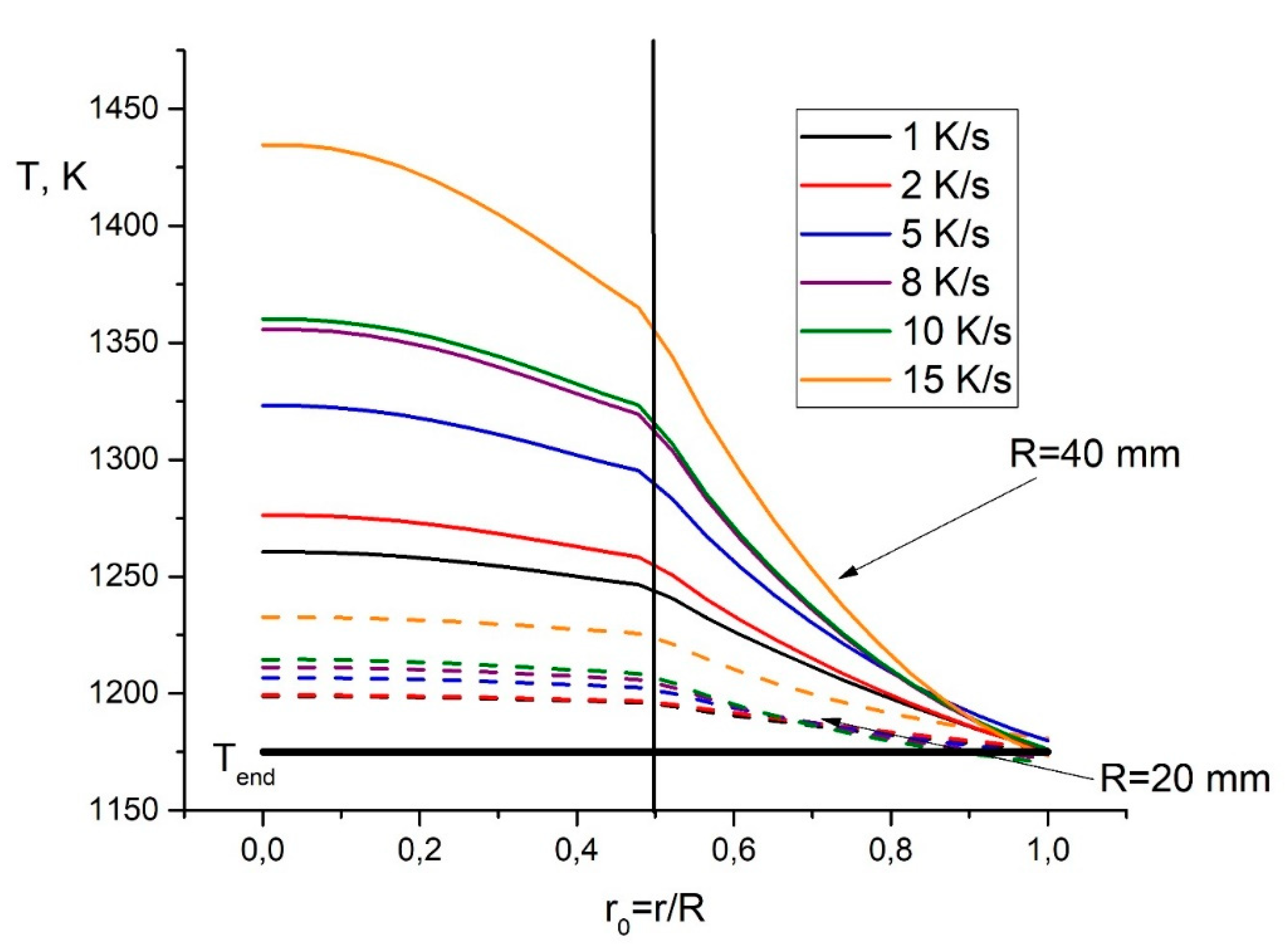
The calculated radial temperature profiles are shown in Figure 2. Heating was carried out to an end temperature of 1675 K, which corresponds to the temperature on the outer surface of the graphite die measured by a pyrometer. It can be seen from Figure 2 that at high heating rates of 15 and 10 K/s, alumina will have a temperature below the temperature of graphite on the outer surface of the die. On the contact surface between the sample and the walls of the die, there is a temperature jump caused by the contact electrical resistance. The entire current flow is concentrated in the graphite die since graphite is a conductive material, in contrast to alumina. For heating rates of 8, 5, 2, and 1 K/s, the temperature in the central part of the sample with a large radius (20 mm) will be higher than the temperature of graphite on the outer surface of the die. This temperature difference can reach 250–300 K for low heating rates of 1 and 2 K/s.

Large temperature jumps were observed in the region of transition from alumina to graphite at high heating rates, but as the latter decreased to 5 K/s and 2 K/s, the jumps also decreased and disappeared altogether at a heating rate of 1 K/s.

For a sample radius of 10 mm, the temperature jumps at the interface between the sample and graphite are much smaller than the corresponding temperature jumps for a sample with a radius of 20 mm. In Figure 2, the behavior of the curves for a sample radius of 10 mm is almost identical to the behavior of the curves of the current distribution as a function of the sample radius in [5].

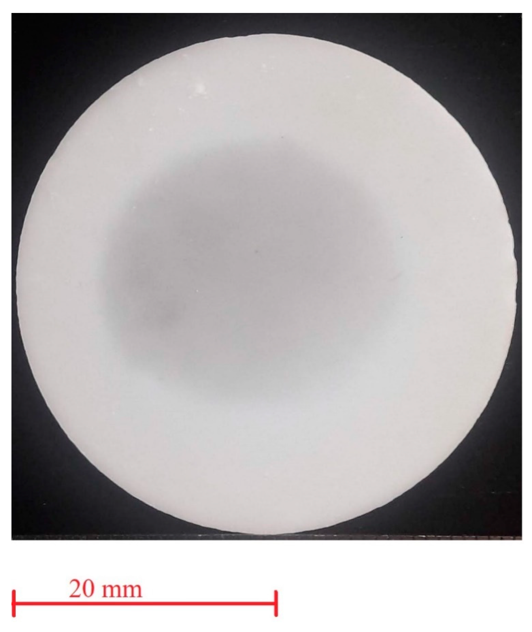
Figure 3 shows a photograph of an alumina sample obtained by SPS. The dark spot in the central part of the sample is due to temperature inhomogeneity and the local conditions of interaction with the surrounding graphite due to slow heating rate.

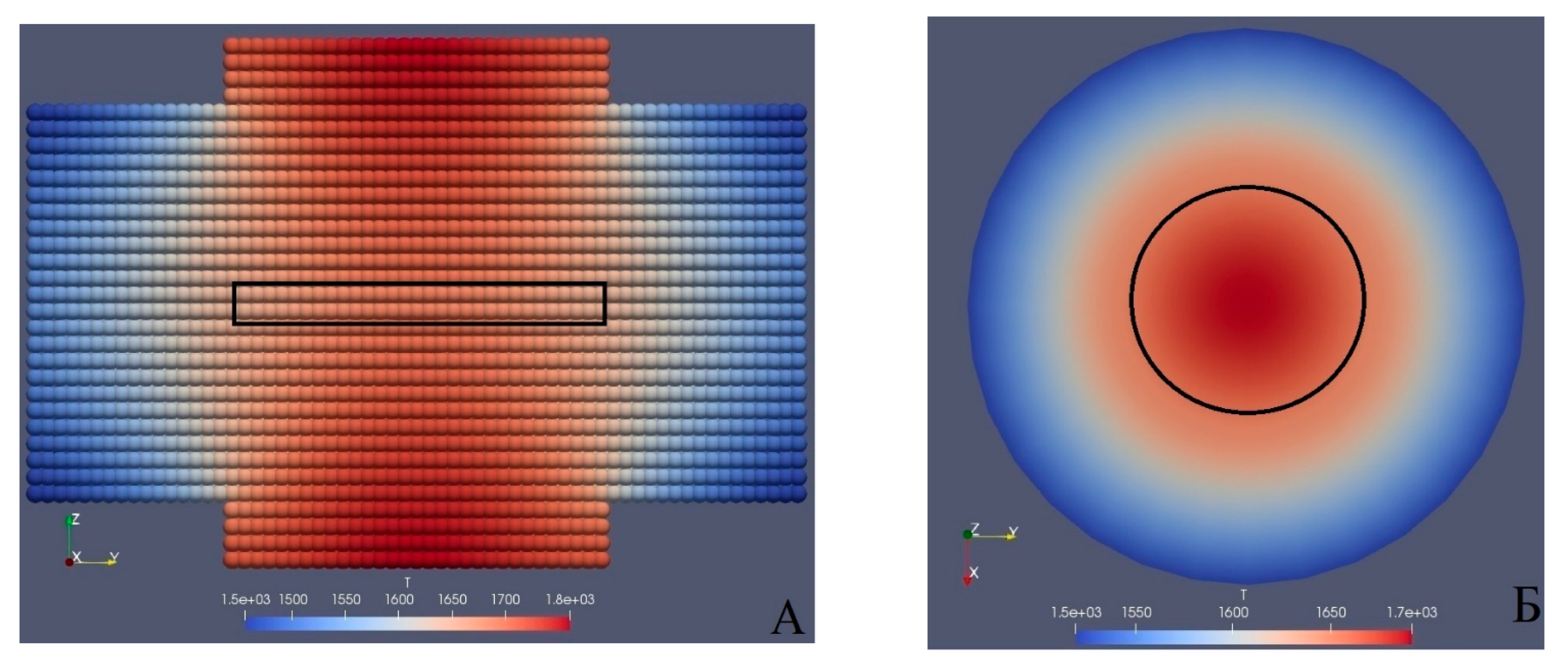
Figure 4 show the calculated temperature distribution in the graphite die and alumina sample under the same conditions as in the experiment in Figure 3. The experimentally observed inhomogeneity in the form of a dark spot at the center of the sample correlates with the appearance of the sample in our calculation in Figure 4B, which shows the calculated temperature distribution in alumina (at the center).

We obtained results for copper samples sintered in dies with radii of 20 and 40 mm. Since copper is known to be a very good electrical conductor, it was expected that copper samples will heat more strongly than the die walls.

Figure 5 shows the radial temperature profiles versus dimensionless radius. The radial temperature distribution in the sample is considered for the moment when the temperature on the outer surface of the graphite die reaches 1175 K, i.e., the temperature to which heating is carried out. It can be seen that for all heating rates, the temperature of copper is higher than the temperature of the outer surface of graphite. Starting at a heating rate of 8 K/s and higher, the temperature in the sample with a radius of 20 mm is about 250 K higher than the temperature measured on the graphite surface. This difference in temperature inside the sample and at the periphery of graphite is due to the fact that copper has better thermal and electrical conductivity than graphite.

It can be noted that the temperature of small (10 mm) copper samples heated at rates of 1 to 5 K/s differs only slightly from the temperature on the outer surface of graphite (solid black line), in contrast to the behavior of the corresponding temperatures during heating of large (20 mm) samples.

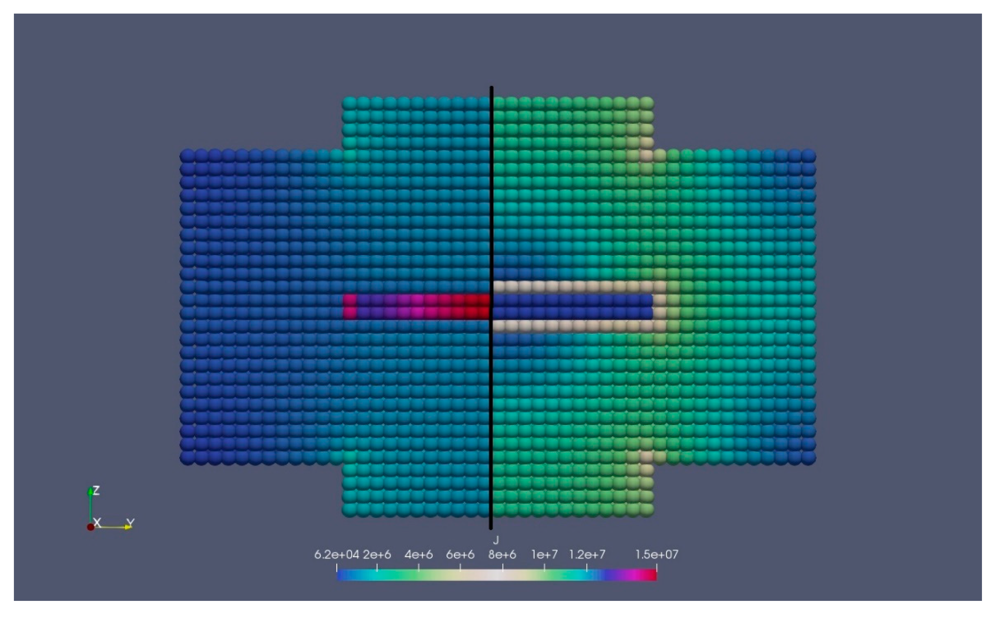
Figure 6 shows the current density distribution in two samples of alumina and copper. Current density plays a major role in heating. It can be seen that the electric current in the die flows around the alumina sample so that the highest current densities are observed at the contact boundary. The alumina sample is in a hot graphite “coat,” which heats it due to heat transfer. If we consider a sample of alumina surrounded by graphite as a defect, then the “coat” around alumina can be explained as pinning a charge on the defect. For copper, the situation is different. The highest current density is observed in the central part of the sample, due to which the copper is directly heated. The current concentration at the edges of the copper can be explained by the skin effect.

As can be seen, for sintering of these two materials with different electrical conductivities, there may be significant inaccuracies in evaluating the temperature of samples from measured temperatures on the graphite die surface.

4. Thick Specimen Model

Prior to this, the results obtained for thin samples were considered, when the thickness of the sample is many times smaller than its diameter. Most often, samples of much larger sizes are required, that is, when the thickness of the sample is comparable to its diameter or larger. Consider the following parameters of the model: (1) outer radius of the die R = 20 mm; (2) sample radius r = 10 mm; (3) two values of the sample height h = 20 and h = 40 mm; (4) die height H = 80 mm; (5) initial temperature T₀ = 300 K; (6) graphite die and graphite punch; (7) alumina and copper samples; (8) heating rates of 8, 5, 2, 1, and 0.5 K/s; (9) the values for heat capacity, thermal conductivity, and resistance are taken from [2] and [4]; (10) the electrical resistance of alumina is temperature-independent (constant).

The results of computer simulation for copper samples are presented below.

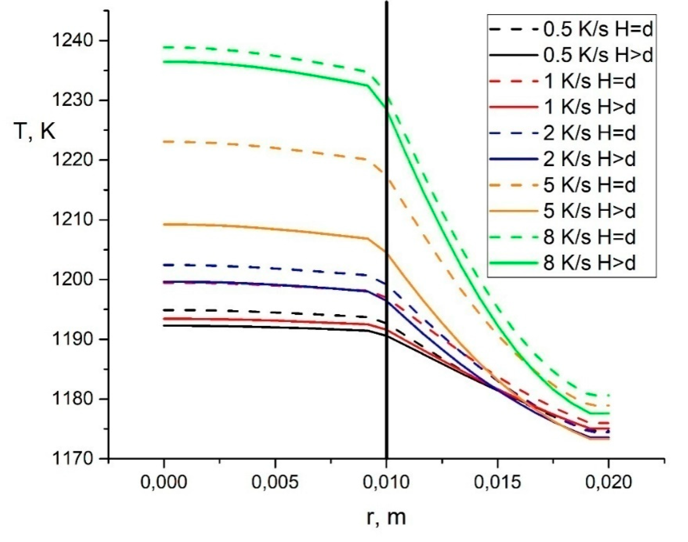
It can be seen from Figure 7 that all temperature distribution curves for samples with a height greater than the diameter are below the temperature distribution curves for samples with a height equal to the diameter. This is natural since samples of greater heights are more difficult to heat. A significant difference between the temperature distribution curves of the samples is observed for a heating rate of 5 K/s. The radial temperature distribution curve at a heating rate of 1 K/s for a sample with a height equal to its diameter coincides with the similar curve at a heating rate of 2 K/s for a sample with a height greater than its diameter. For all curves, the temperature in the central part of the sample is higher than the temperature at the periphery, where there is contact with the graphite die. As in the case of thin disk samples, the following trend is observed: the higher the heating rate, the higher the temperature difference at the center and at the periphery of the sample.

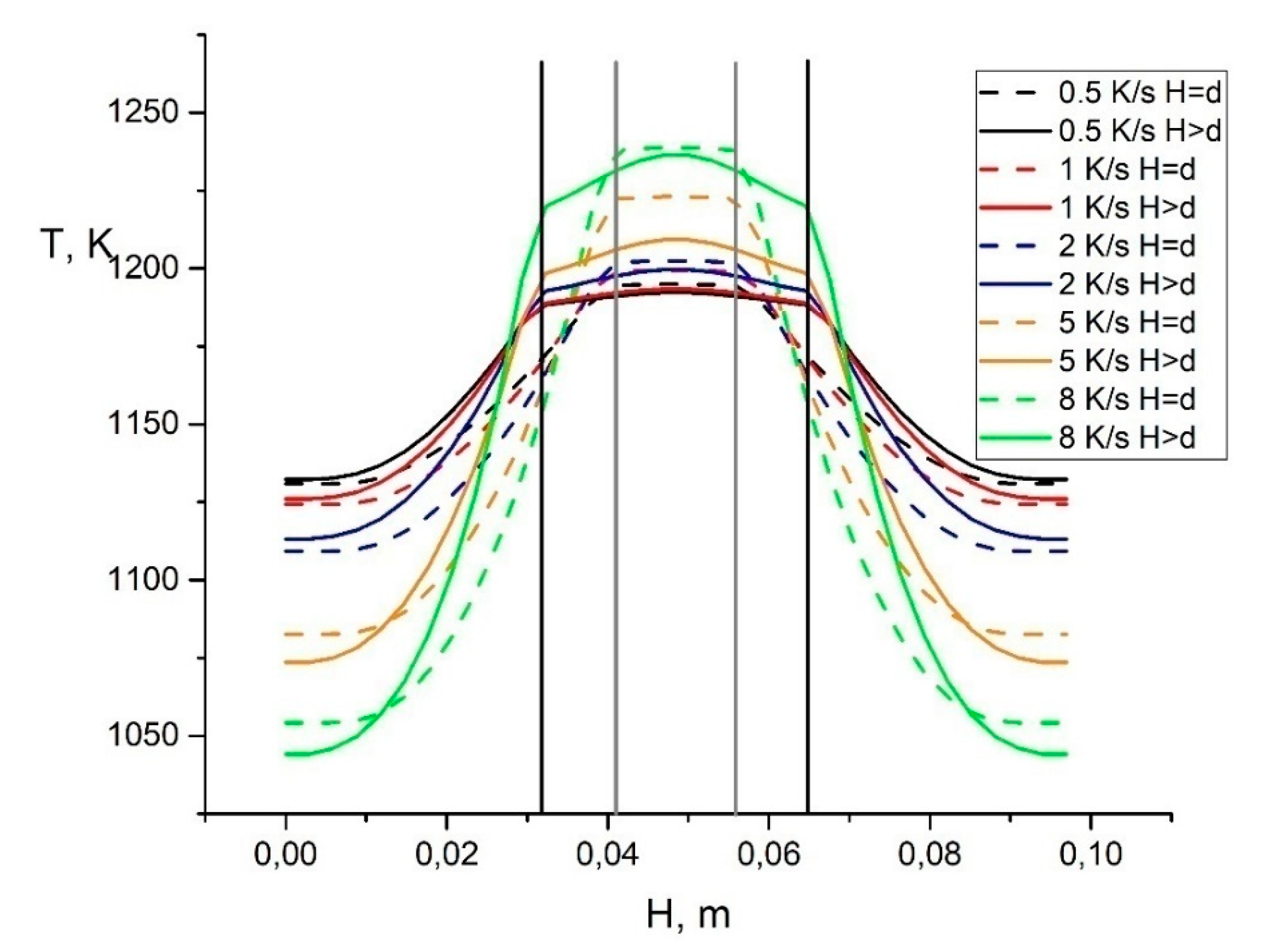
Figure 8 shows the temperature distribution in samples along the Z axis. It can be noted that at a high heating rate, the temperature of the samples in contact with the punches is lower than the temperature in the central part. As expected, low heating rates of 0.5 to 2 K/s promote uniform heating of the samples.

The results of computer simulation for alumina samples are presented below.

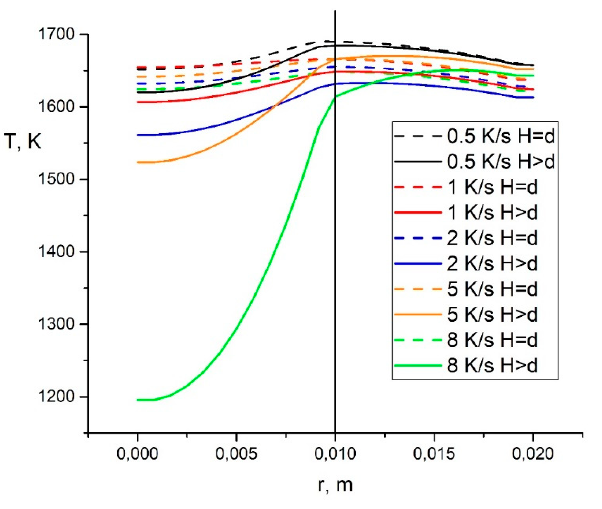
The radial temperature distribution curves in Figure 9 show that at high heating rates for alumina samples with a height greater than the diameter, the sample temperature is always lower than the temperature of the graphite die.

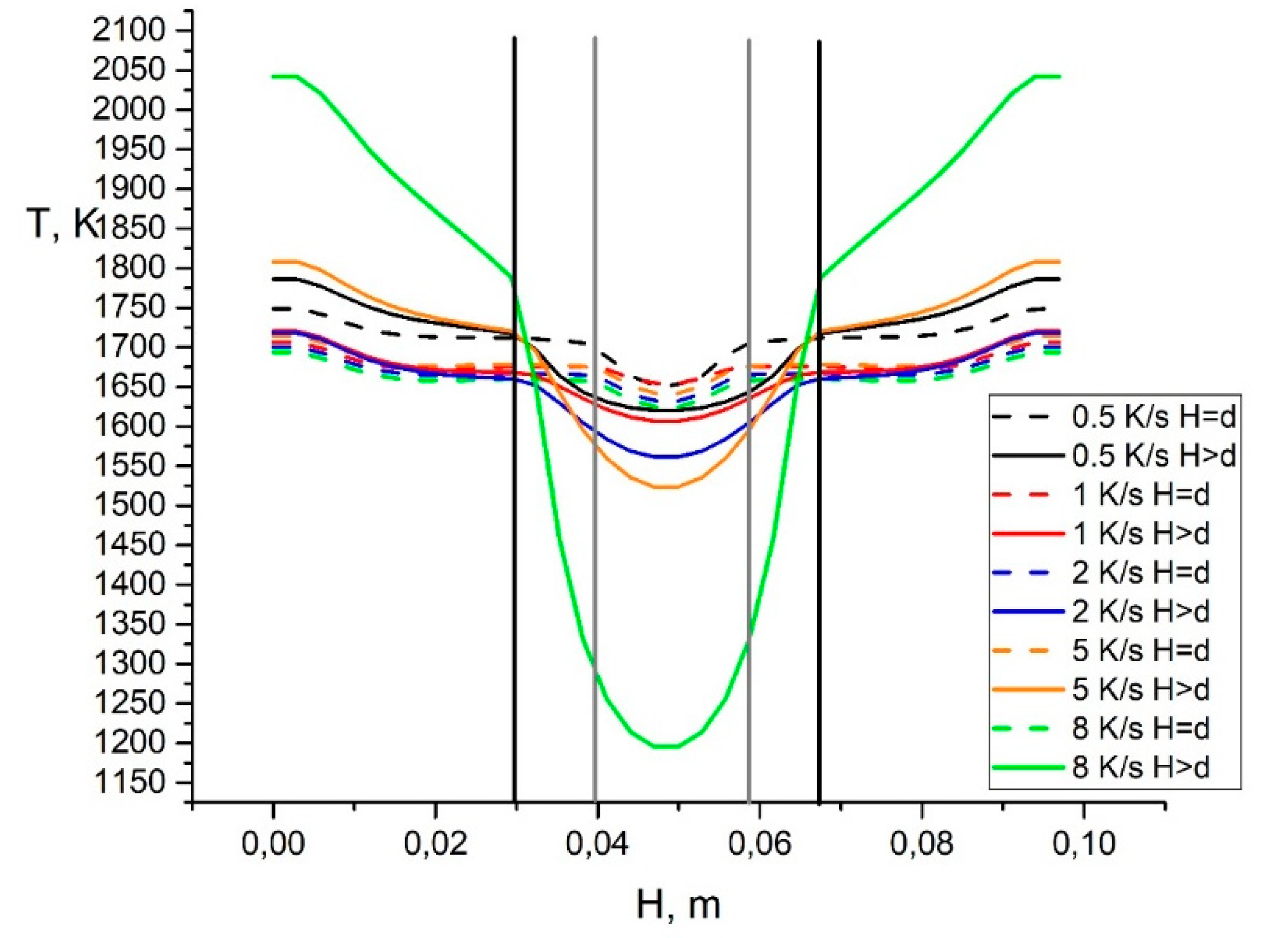
Figure 10 shows the results of calculating the change in the temperature of an alumina sample along the Z axis. At high heating rates in a sample with H = 4r, there is a strong “dip”—a decrease in temperature in the central part, which is clearly visible at a heating rate of 8 K/s. The central part of all samples in Figure 10 remains unheated even at low heating rates.

The calculations obtained for Figure 9 and Figure 10 made it possible to create a method for the manufacture of large-size materials under SPS conditions [6].

5. Conclusions

A computer program has been created for calculating the thermal fields in dense samples of copper and aluminum oxide surrounded by graphite, and at various rates of heating by an electric current.

It was found in the calculations that significant temperature gradients are observed at the boundaries of a thin sample of aluminum oxide and graphite, which are especially noticeable at large sample radii. The dependence of the temperature of the alumina sample on the value of the radius and heating rate is found. The heating rates are found at which the temperature values at the center of the samples and at the periphery of the graphite practically coincide.

Calculations have shown that for an electrically conductive material, copper, the sample temperature is always higher than the mold wall temperature. This difference becomes greater the higher the heating rate, and significantly depends on the size of the radius.

A slight drop in temperature is observed only at the boundaries of copper with graphite punsons. This makes it possible to predict the possibility of obtaining large-sized workpieces from conductive materials.

In aluminum oxide, the calculated radial temperature decreases with increasing sample height and has dips in the center, which strongly depend on the heating rate.

Since in experiments the temperature is measured not in the sample itself, but on a graphite mold, in order not to deteriorate the quality of the products obtained, it is very important to know how large the deviations of real temperatures from the measured ones are. Calculations have shown that temperatures on the surface of graphite molds differ significantly from the temperatures of sintered samples, both for conductive and insulating materials and depend on the heating rate.