Ion Acceleration in Multi-Fluid Plasma: Including Charge Separation Induced Electric Field Effects in Supersonic Wave Layers

School of Mathematical and Natural Sciences, University of Arkansas, 346 University Drive, Monticello, AR 71656, USA
†
Current address: Science Center, 397 University Drive, Monticello, AR 71656, USA.
Plasma 2020, 3(3), 117-152; https://0-doi-org.brum.beds.ac.uk/10.3390/plasma3030010
Submission received: 26 March 2020
/
Revised: 12 August 2020
/
Accepted: 16 August 2020
/
Published: 21 August 2020
Abstract
:The need to understand the process by which particles, including solar wind and coronal ions as well as pickup ions, are accelerated to high energies (ultimately to become anomalous cosmic rays) motivate a multi-fluid shock wave model which includes kinetic effects (e.g., ion acceleration) in an electromagnetically self-consistent framework. Particle reflection at the cross-shock potential leads to ion acceleration in the motional electric field and thus anisotropic heating and pressure in the shock layer, with important consequences for the multi-fluid dynamics. This motivates development of a multi-fluid model of solar wind electrons and ions treated as fluid, coupled self-consistently with a small population of ions (e.g., pickup ions) dynamically treated as individual particles. Consideration of both the time dependent and steady state regimes, indicate that such a multi-fluid approach is necessary for resolving the, Debye scale, particle reflecting cross-shock potential and subsequent dynamics. To study charge separation effects in narrow, supersonic wave layers we consider a reduction of the system to the steady state for cold ions and hot electrons and find two types of solitary waves inherent to the reduced two-fluid system in this limiting case.
1. Introduction
Investigations of multiply reflected ion (MRI) acceleration at perpendicular shocks, where ions are treated as test particles, with detailed trajectories calculated from the Lorentz force equation, have found MRI to be an efficient mechanism capable of energizing ions up to energies on the order of ∼100 keV, as needed for injection into diffusive shock acceleration mechanisms [1,2,3,4,5] which further accelerate them to become the so-called anomalous component of cosmic rays. Much of this work treats the electromagnetic fields as fixed and ions as test particles. For an improvement, we have presented a two-fluid solar wind (SW) simulation with pickup ions (PUIs) coupled quasi self-consistently via inclusion of the PUI anisotropic pressure—calculated directly from their precisely tracked trajectories [6]. Continuing this work, here we consider a self-consistent inclusion of the back-reaction, due to ion acceleration, including their action on the electromagnetic fields as well as their anisotropic pressure. The possibility of self-consistently including ions, treated as particles (in a manner similar to particle-in-cell or PIC codes), using a 1-fluid MHD (magnetohydrodyamics) model, with source terms included to account for shock accelerated ions, has been rejected because, as considered below, only a multi-fluid plasma treatment can resolve important charge separation effects in supersonic wave layers.
When charge separation gives rise to particle reflecting electrostatic fields, resolution on electron Debye scales is necessary to include important plasma dynamics. For example, studies of adiabatic solitary waves [7] and shock surfing at a two-fluid plasma model [8], indicate that the cross-wave electrostatic field structures form on electron Debye scales. At such a fine scale, electric fields provide important force sights where suprathermal ions gain energy by acceleration along the motional electric field after reflection from an electrostatic cross-shock potential (CSP), thus providing a dissipation mechanism for super-critical collisionless shocks, which can explain some observations. For example, reflected and accelerated pickup ions can explain the cooler than expected solar wind observed by Voyager 2 downstream of the heliospheric termination shock [1,2,4,9,10].
Such observations and simulations indicate that electrostatic solitary waves (ESWs) are dynamically coupled to shocks in multi-fluid plasmas [11,12,13]. In this context, we pursue the development of a self-consistent fluid dynamics model that can incorporate the effects of reflected particles, in particular for shock-surfing pickup ions. Indeed, our two-fluid hybrid model, including dynamically coupled ions, treated as test particles [6], required a multi-fluid treatment without the common assumption of quasi charge-neutrality (e.g., used consistently in [Tidman and Krall, 1971] [14]) since particle reflecting electrostatic structures arise from charge separation when ion and electron densities are perturbed from balance in narrow wave layers.
As an illustrative simplification of the complex multi-fluid system, we treat the special case of cold ions and hot electrons in the steady state of the wave frame, while noting that such plasma conditions may be appropriate e.g., for modeling electrostatic solitary waves (ESWs) in the electron foreshock region of Earth’s bow shock where intense Langmuir waves are observed to be generated there by suprathermal electrons [11]. By solving the resulting coupled set of ordinary differential equations (ODEs), via numeric parameterization of the set, we find both accelerating and decelerating solutions of ESWs associated with both electrostatic potential hills and wells, much like the two types of ESWs observed by Geotail near Earth’s bow shock [11].
Motivation for the Development of a Multi-Fluid Plus Kinetic Ions Plasma Model
The need for development of multiple-scale plasma simulation methods has become increasingly evident [15,16]. For example, in heliospheric plasma, resolution over multiple scales is necessary to describe events where large amounts of electromagnetic energy is converted, over short times, into kinetic energy. Such events are ubiquitous throughout space and occur e.g., at magnetic reconnections such as those observed in Earth’s magnetosphere during magnetic storms. The diffusion processes (visible as the aurora Borealis) that cut and reconnect magnetic field lines during these events occur on electron kinetic scales [17] and yet transfer explosive amounts of kinetic energy into the plasma particles, driving the large scale physics of magnetohydrodynamics (MHD). In addition, diffusion processes at shock waves, such as shock drift acceleration (SDA) [18] and shock surfing acceleration (SSA) [2,3], discussed above, serve as pre-acceleration for efficient injection into Fermi-acceleration and ultimately effect global, MHD scale structures. Meanwhile, proper descriptions of the thermal diffusion at collisionless shocks by SDA and SSA requires resolution across electron up through ion kinetic scales.
For heliospheric scales, where regions of interest are on the order of astronomical units, plasma simulations are typically computed with MHD codes [19]. Although such high resolution MHD methods are very computationally efficient and allow for step-jumps e.g., at shocks, these codes invariably assume local charge neutrality and some form of idealized Ohm’s law, so that Alfven waves and magnetosonic waves dictate the characteristic scales of MHD.
On the other end of the computational spectrum from MHD, electron kinetic scales, characterized by the electron Debye length and plasma frequency, can be well simulated with PIC codes, such as VPIC (Vector Particle-In-Cell), which was employed to study the nonlinear evolution of ion ring-beam distributions in low beta plasmas [20]. As multi-threaded computational power increases, PIC codes may well emerge as the best way to model plasma evolution throughout the global helioshere. Nonetheless, PIC codes are essentially brute force methods where every superparticle is tracked and their kinetics simulated via the interaction of their trajectories under the Lorentz force, with Maxwell’s equations. Thus, the simplicity and fine scale resolution of PIC comes at the high cost of computational burden. In other words, PIC code simulations require lots of computer power and time to run. Thus, we seek to develop a multi-fluid method suitable for modeling SSA, and the like, across the large scale termination shock (TS,) a method that through the use of fluid equations is less computationally expensive than PIC, but that can properly resolve important ion dynamics which cannot be resolved by MHD.
Multiplying the continuity equations (see e.g., [21]) for electrons and ions by their fundamental electron charge e and summing yields the charge continuity relation
where q and are the total charge density and current. The usual neglect of the displacement current in magneto-hydrodynamics (MHD) yields
in Ampere’s law implying that and thus that the charge density q is everywhere constant, meaning that a 1-fluid MHD approach, which assumes charge neutrality everywhere, cannot resolve the cross-shock potential (CSP) inducing charge separation in the shock layer. As outlined below, in order to resolve charge separation, we present a two-fluid plasma model which includes a third population, composed of candidate ions which we term as shock accelerated particles (SAPs) likely to be MRI accelerated, to be treated kinetically as quasi-test particles–meaning that for the duration of a time-step (on the plasma fluid scale) the electromagnetic fields are fixed and the trajectories of the SAPs, along with their associated stress and energy tensors, are calculated. The SAP tensors are then fed step-wise into the 2-fluid plasma model as source terms. A brief description of shock surfing acceleration, with implications for source terms follows.
Multiply reflected ion (MRI) acceleration can occur when plasma is suddenly decelerated at a shock wave where the more massive ions on average, having more momentum, are able to penetrate further into the density pile-up immediately downstream of the shock than do the less massive electrons. The subsequent charge separation results in the formation of a cross-shock potential (CSP) which acts as an electrostatic barrier to incoming ions. Some ions incident at the shock with insufficient shock-normal component of velocity to overcome the CSP will be reflected. Reflected ions, which can be thought of as kicked out of the SW frame where electric fields are negligible, are acted on by the motional electric field (directed tangentially to the surface of a perpendicular shock) and can thus be significantly energized by MRI acceleration.
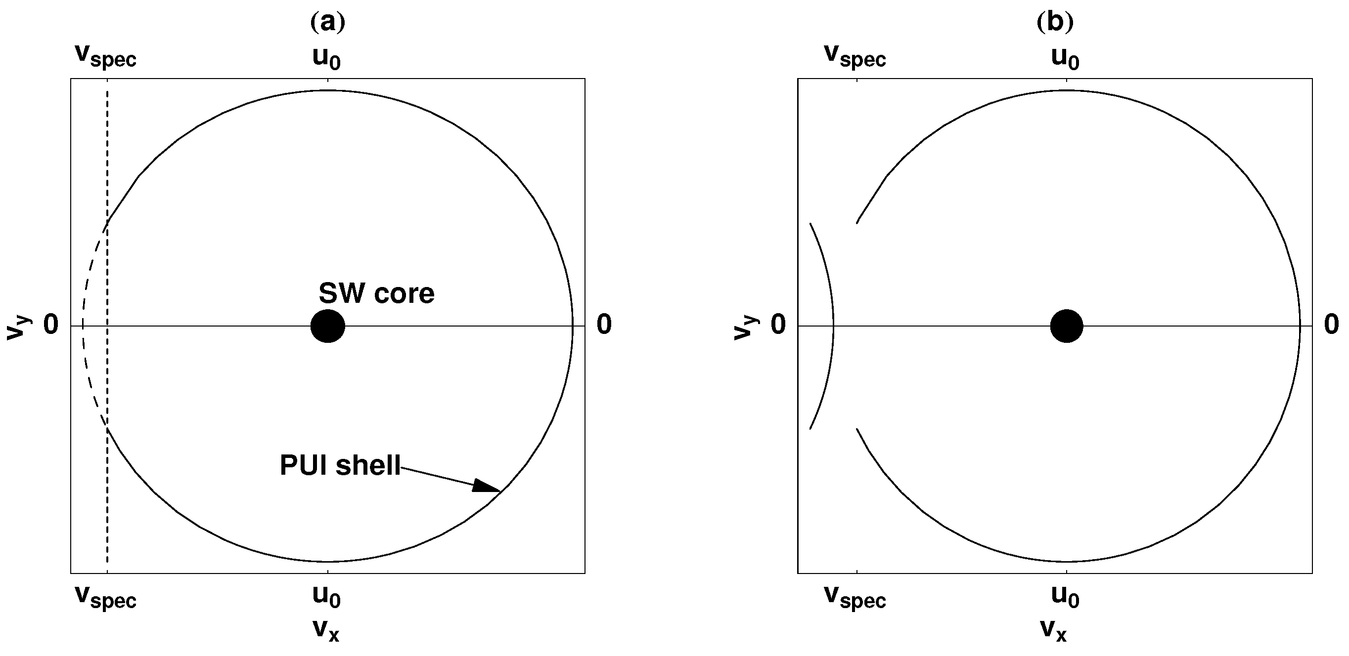
As illustrated in Figure 1 (which illustrates a shell distribution where the entire portion of the shell satisfying has undergone a single reflection) ion reflection can occur when
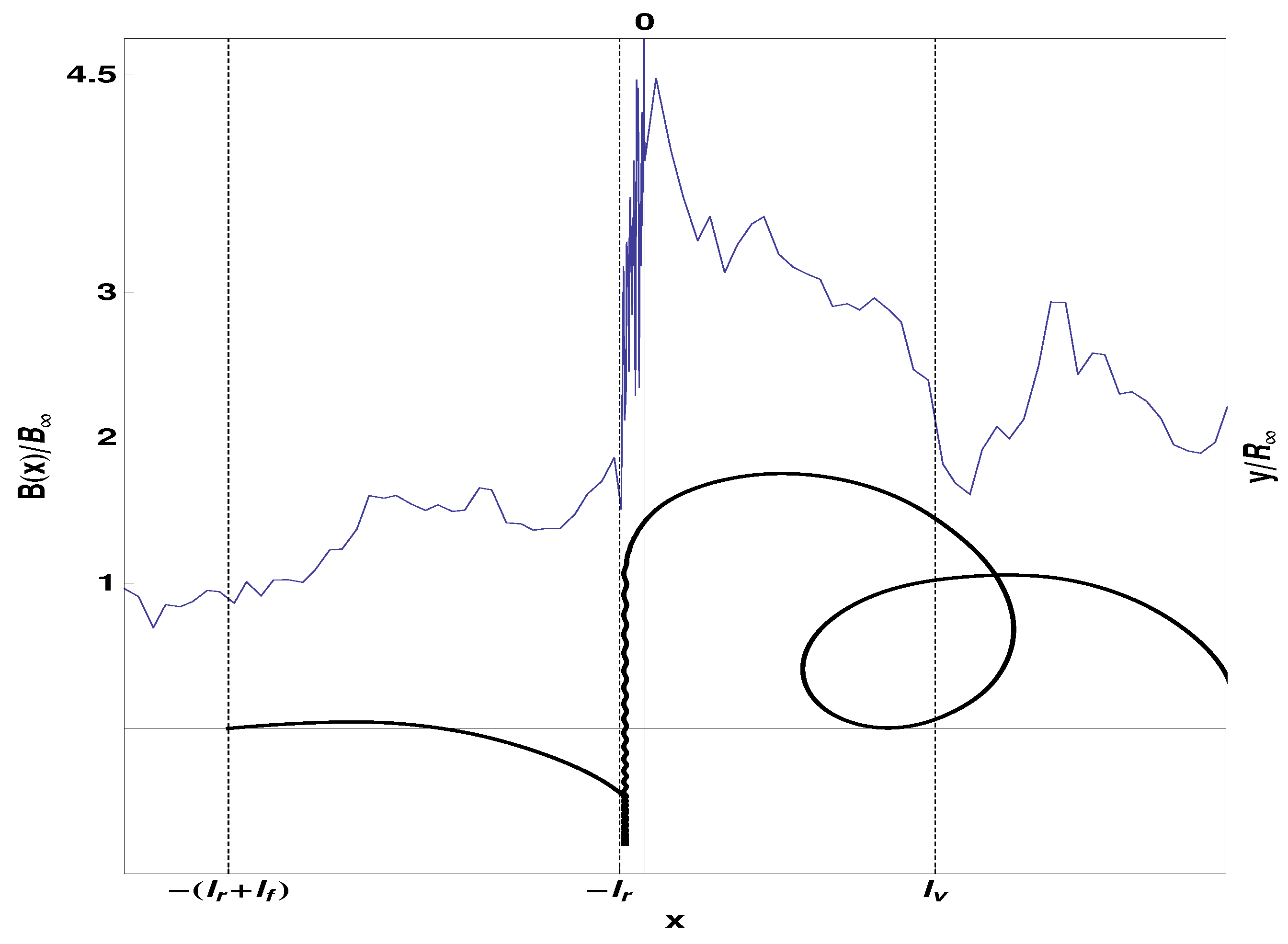
i.e., when the ion’s x-component of velocity is insufficient to overcome the CSP barrier. For a PUI distribution incident on a simple step-function shock structure with a vanishingly narrow ramp width (such as considered by [2]), the entire portion of the distribution satisfying the reflection condition will undergo one or more reflections, resulting in very strong energization of the downstream PUIs. On the other hand, the main ion population, the SW ions which lie on a relatively cold Maxwellian core distribution (the heavy central dot depicted in Figure 1) are transmitted downstream of the shock with virtually no reflection. In a recent article [1] we have performed a test-particle simulation of the termination shock (TS) showing that MRI acceleration can also be important at shocks with fairly large ramp widths but that still posses sufficiently narrow fine structure to support reflection. An example of a single PUI undergoing shock surfing acceleration (SSA) in the fine structure of the quasi-perpendicular TS ramp is illustrated in Figure 2, which shows how some ions experience multiple reflection and thus strong energization due to SSA in the ramp. Thus motivated by the important role the shock structure plays in ion acceleration, we seek a 2-fluid plasma model that will allow us to resolve fine details of the electric and magnetic fields in the local vicinity of the shock.
There are several important features of MRI acceleration that the 2-fluid plus source terms model must include. For example, as depicted in Figure 3, ion reflection at the shock ramp is expected to perturb state variables such as pressure and density (represented by the arbitrary perturbation quantity in Figure 3). Furthermore, our simulations [1] have shown that PUI pressure behind the termination shock can be highly anisotropic.
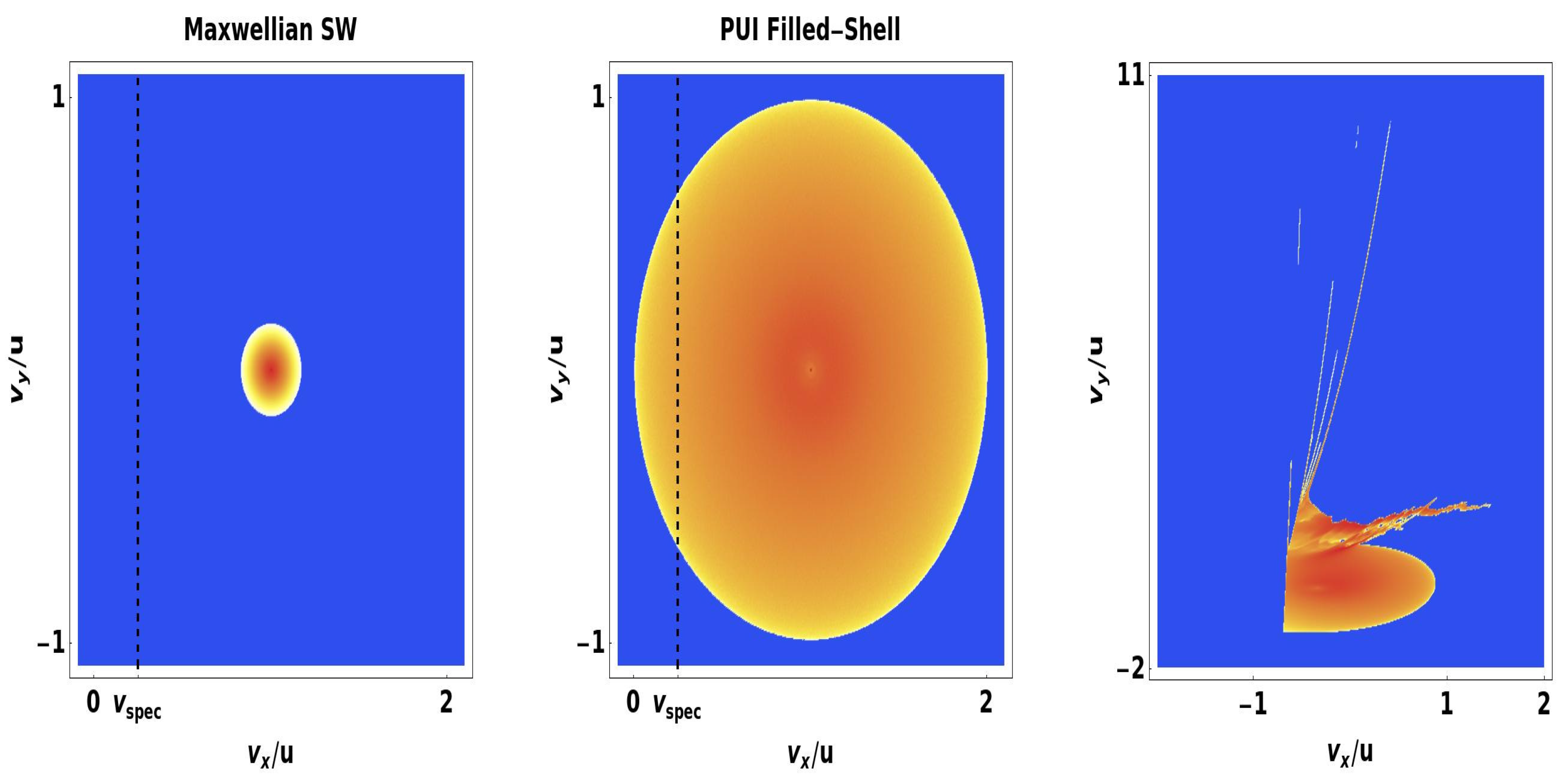
Figure 4 illustrates ion distributions ahead of and just behind the TS model. Note that virtually none of the upstream Maxwellian SW distribution lies to the left of the velocity , whereas a significant portion of the upstream PUI filled-shell does lie to the left of (i.e., in the reflecting region of velocity space). We have shown, in test-particle calculations, that (cold) Maxwellian distributions incident on a narrow, perpendicular shock pass downstream virtually unreflected, as expected. This justifies the assumption employed below in the construction of our numerical model that the 2-fluid SW is Maxwellian and isotropic everywhere. The right hand panel of Figure 4 is the phase-space density plot of an MRI accelerated PUI distribution just behind the TS-model and it is clear that this distribution is anisotropic with important non-zero off-diagonal terms in the associated PUI pressure tensor.
The up and downstream, normalized PUI (or SAP) pressure tensors associated with the middle and right-hand panels of Figure 4 are
respectively, which shows MRI enhancement of the component as well as the formation of shear pressure terms .
The two part description of the total ion distribution considered above comes from basic ideas about how PUIs are formed from interstellar neutrals ionized in the SW [2,22], and should suffice for the simulation model considered here. The numerical generation of more realistic initial conditions, however, could be readily deployed from kappa-distributions by noting that the MRI acceleration candidate ions (such as PUIs) must reside in the high energy tail of the ion kappa-distribution, whereas the cooler, isotropic SW component must come from lower velocity, Maxwellian like, interior of the kappa-distribution. Evidently, such kappa-distribution types occur naturally, since more energetic plasma particles in the SW also have further reduced ‘collision’ frequencies for scattering via Coulomb interactions [23]. Thus, instead of being thermalized onto Maxwellian distributions (as with a typical gas), the high energy portions of populations are generally known, instead, to be well described by (and remain on) power laws having the form for the high velocity regime (or power law tail) of their distributions [24]. The description of the SW environment, as characterized by kappa-distributions, has been shown to be consistent with a statistical mechanics based fluid description of ‘collisionless’ plasmas, making this approach highly attractive and theoretically well supported [25]. For Example, the validity of both theory and observations of kappa-distributions in the SW has been supported by Yoon, who develops a kinetic treatment including electrostatic Langmuir turbulence, and finds by rigorous implication, that SW electrons can be well described by kappa-distributions, consistent with observations of the quiet time SW at 1 AU [24].
Widely in the literature, it is evident that charged particles in the SW environment tend to follow a ‘rich get richer’ scheme whereby the more energetic particles are the ones risen to even higher energies by a wide variety of acceleration mechanisms including MRI acceleration and SDA and various other stochastic acceleration mechanisms to name several. Furthermore, the shock accelerated particle (SAP) candidates for MRI, as considered above, need not be PIUs necessarily. The SAPs need only reside initially within the high energy tail the ion distribution. Since the SW environment in general is well described by kappa-type distributions, while prescribing an initial, isotropic plasma as given by a Maxwellian core (corresponding to the interior or low energy regime of a kappa-distribution) together with a suprathermal tail (corresponding to the high energy regime or tail of a kappa-distribution,) we can note the model considered here could also be applicable for simulating ion acceleration at interplanetary shocks, such as coronal mass ejection driven shocks or planetary bow shocks, though here we are interested in MRI acceleration of PUIs at the quasi-perpendicular TS. Thus, with these ideas in mind, we seek to include the formation of an anisotropic ion distribution in the shock layer via the inclusion of source terms in a two-fluid plasma model as described below.
2. Materials and Methods
2.1. Two-Fluid Solar Wind Plus Kinetically Treated Shock Acceleration Candidate Kinetic Ions Numeric Model
We develop a quasi-self-consistent system composed of a core two-fluid plasma solar wind (SW) background, which is acted on by a small population of ions to be dynamically treated as super-particles (similarly to the way are ions are treated in particle-in-cell (PIC) codes where the term super-particle implies that each PIC particle represents, on average, an arbitrary number of real particles) that are self-consistently coupled to the core SW. We are interested in the case where a small, energetic population, denoted as shock acceleration particles (SAPs) which comprise the population of candidates that can experience multiply reflected ion (MRI) acceleration due to reflection from a cross-shock potential (CSP) leading to ion acceleration in the motional electric field. A two-fluid description is derived to calculate the back reaction on the fields, in essence creating a feedback loop between suprathermal shock accelerated particles (SAPs) with SW electron and ion fluids.
There are two distinct characteristic scale regimes involved in this development: long time and length scales () associated with the description of the two-fluid core SW plasma, and short time and length scales () associated with SAP dynamics (particularly within the narrow shock structure). The prescription here, for constructing a closed system that can be solved numerically, is to treat the electric and magnetic field and as constant for each time period during which we solve the motion of the SAP candidate ions (treated in a manner much like particle-in-cell (PIC) codes); the pressure and heat flux tensors resulting from the detailed ion trajectories are then feed into the 2-fluid plasma equations as source terms; the 2-fluid equations are used to update the values of and over the longer time scale and the process is iterated. Below we present a system ready for such a numerical treatment.
The derivation of the plasma fluid equations is followed from Boyd and Sanderson, Plasma Dynamics [21], Chapter 3 (from now on referred to as B&S), however instead of treating the system as two groups of particles, ions and electrons (labeled in B&S by ‘+’ and ‘−’, respectively), we treat the system as composed of three groups of particles, labeled {s, a, e}, which are solar wind (SW) ions, shock acceleration candidate ions and electrons, respectively. The shock acceleration candidate ions (e.g., pickup ions (PUIs)) may compose between 0 to 20% of the total ion population and are kept separate since they will be treated as SAP superparticles.
Definition 1.
Ion number density composed of the SW ions plus SAP candidates is
and the electron density is .
The charge density is
and ion fluid velocity is
The current density is
Here m is the ion mass (which for now is a proton mass), e is the electron/proton charge. The random (thermal) velocity of each species is
Pressure tensors are defined as
and the heat tensors are
where, as per the B&S convention, species labels are suppressed to simplify the notation.
Since, in (5), both SW ions and SAP ions have thermal velocities defined with respect to the common ion bulk velocity, the total ion pressure tensor can be written as the sum of two partial pressures
We make the closure assumption that SW ions and electrons can be treated everywhere as thermalized, isotropic distributions such that
and
The shock accelerated particle (SAP) pressure is taken to be composed of an isotropic and anisotropic part,
and has a nonzero heat tensor . All fluid equations are constructed from the transfer equation
where the closure assumption that collision terms are negligible has been made. Continuity equations result from (12) when .
Ion momentum, , (i’th component)
where for ions
(species labels suppressed) Electron momentum (ith component)
where for electrons
Taking , (16) becomes
Ion energy
where for ions we have used
Electron energy
where for electrons
since . Taking , (21) becomes
With the Maxwell curl equations,
Equations (13), (14), (18), (19), (22) plus (23) and (24) form a set of 16 equations in the 16 unknowns to be solved numerically by a fluid code, and the included sources terms and are to be determined by a kinetic treatment of the SAP candidate ions.
2.1.1. Conservation Form of the Two-Fluid Plasma Equations
2.1.2. Dimensionless Forms of The Equations
To prepare the equations for numerical discretization define the following dimensionless variables:
where L is an arbitrary length scale and, as justified below,
and the ∞ label indicates the constant far upstream (boundary) values for the state variables. In addition, note that the dimensionless ion pressure can be expressed in terms of ion partial pressures
The dimensionless derivatives of dimensionless state variables take the form
To simplify the notation for the two-fluid plasma system expressed in dimensionless form, it is useful to define the following dimensionless plasma parameters
which are expressed in terms of the far upstream ion gyro-frequency, ion plasma frequency and ion gyro-radius defined as
respectively. In writing the following dimensionless equations it is convenient to drop over-bars and take it as understood that all variables and derivatives dimensionless. In addition, note that the components of the dimensionless bulk velocities for the ions and electrons are given by
respectively. In dimensionless form the continuity Equations (13) become
Ion momentum (14) becomes, (ith component)
Electron momentum (18) becomes, (ith component)
Ion energy (19) becomes
Electron energy (22) becomes
The the total momentum Equation (25) becomes
where the dimensionless Maxwell stress tensor is
The total energy Equation (26) becomes
The Maxwell Equations (23) and (24) can also be expressed in dimensionless form as
where
The Poisson’s equation () can also be expressed in dimensionless form as
2.2. Special Case: Quasi-One Dimensional, Exactly Perpendicular Shock
As an initial case, limit variations to the shock normal direction (x-direction) so that
Consider an exactly perpendicular shock configuration, with
where the plasma flow at the far left (upstream) boundary is
as . The assumption of charge neutrality can be imposed at the left boundary so that the dimensionless boundary conditions at are
The fluid plus Maxwell’s equations can now be expressed in the dimensionless form
where the state vectors in (45) are
where The two remaining equations are
from the electron momentum (34). Thus, Equation (45) plus (46) and (47) form a complete system ready for the construction of a numerical solution. For example, (46) and (47) can be used to eliminate the electric field components directly. Furthermore, since none of the plasma state variables depend on the z-components of velocity, we assume and . In fact examination of the steady state system (presented below) indicates that if at the left boundary () then the z-component of bulk velocity will remain zero, i.e., we can view the z-direction as ignorable for the special case under consideration.
An alternate ‘quasi-conservative’ form of system (45) plus (46) and (47), expressed as
can be formed by swapping out the ion momentum and energy equation with the total momentum and energy equations in the conservation forms given by (37) and (38), where state vectors in (48) are written as
The above system must be supplemented by the electron equations
where (51), the quasi-conservative form of the electron energy, results on summing the x-component electron momentum (46) and the electron energy equation. Additionally, the system (48) must be supplemented by the remaining non-conservative components of Maxwell’s written as
In the above treatment, the system is taken to be composed of three constituents: the core SW electron fluid and two ion components, including core SW ion fluid with SAP candidate ions interacting and interlaced over two time scales. Here, the core SW fluid components are assumed to be dynamically amenable to longer simulation time steps Whereas resolution of the SAP dynamics could require shorter time steps so that where . The SAP population is to be treated in the model as superparticles with their trajectories governed by the Lorentz force as is done in PIC codes, and here using as the SAP simulation time step. In view of Equations (1) through (8), which are consistent with the total ion pressure being treated as the sum of ion partial pressures, the model is technically just that of a two-fluid plasma. So how is the ‘third’ fluid component, for the SAP candidates, to be included in the simulation model through their treatment as superparticles? These same defining equations provide the answer. After each time step evolution of the fluid over the longer scale The fluid and electromagetic field parameters can be held fixed while the SAPs are iterated through n time steps as test particles. Thus, SAPs are evolved step-wise through the longer time step , after which their fluid parameters can be directly calculated from their superparticle distribution averages. These directly averaged SAP fluid parameters (, , etc.) can be incorporated or fed into the two fluid plasma description, at the beginning of each long scale time step, through use of the fluid definitions as prescribed by Equations (1) through (8). Although, to minimize the effects of unnatural distortion that may arise from the prescribed use of superparticles essentially as source terms in a two-fluid model, the anisotropic SAP candidate population should perhaps be kept small. For example, taking PUIs at the TS to be 10% of the total ion population, a reasonable lower bound estimate [26], then the initial normalized ion density would be as required by our normalizations. Even lower percentages of SAP candidate ions could be reasonable, especially if we consider interplanetary shocks on the order of 1 AU or so from the Sun where we might assume that even lower ion percentages reside in the suprathermal tail of the total ion distribution.
Steady State Equations for 1D Case with Perpendicular Magnetic Field
In the steady state and (48) reduces to
From which it is seen that several integrals of the motion are readily obtained. It turns out that for the special case under consideration there are nine algebra relations (i.e., 9 integrals of the motion) that can be obtained from the plasma system in the steady state (SS). The variables of the special case system under consideration are for a total of 11 unknowns. This means that, in principle, the SS system can be determined from a coupled pair of ODEs in two of the unknowns. Having solved the coupled ODEs, the remaining unknowns can be found from the algebra relations and the system thus completely determined. The first four algebra relations are
The first two SS relations, expressed in (55) above, follow from the continuity relations (i.e., first two components of (54)) and the boundary conditions (44). The remaining two constants of the plasma system, expressed by (55) follow from the Faraday relation given by the last component of (54) along with the y-component of electron momentum expressed by (50). The third, fourth and fifth components of (54) express conservation of total momentum and energy in the SS as
where (44) and (55) have been applied and is the total (dimensionless) pressure at the upstream boundary which is taken to be completely isotropic there. The equation of state for adiabatic electrons
follows from (51) and (55). Using algebra relation (57) in Poisson‘s’ Equation (41) yields
which, upon using (55), is also given by the y-component of the ion moment i.e., the fourth component of Equation (54). This demonstrates explicitly that the Poisson’s equation is a corollary of the plasma fluid equations and the Maxwell curl equations. Several additional relations can be obtained by systematic substitution of the algebra relations (55)–(58) back into the SS forms of the non-conservative equations given by (45). As mentioned, this process recovers the Poisson’s Equation (60) above along with several ODEs in the electron density
from which we can recover an additional algebra relation
where . Using (55), (60) and (61) can be written as
By using (56) and (58) to find , the coupled set of ODEs (65) can (in principle) be solved numerically and the steady state solution thus determined.
3. Results
3.1. Steady State, 1D Two-Fluid Plasma System with Cold Ions
Though reduced to the steady state, the above coupled set of ODEs, nonetheless, represents a considerable challenge for use in evaluating valid solutions. Thus, as an initial step, we consider a further simplification to the case of cold ions and hot electrons. Previously we have solved such a simplified two fluid system as an integral over a single component of the plasma velocity [27], which has the advantage of providing an exact (albeit numerical) solution of the wave structure. Here we solve for the wave structure by introducing a parameterization of the coupled ODEs. Though this coupled ODEs method might not be exact as the integral form, it has the advantage of being extensible for use in more complex cases, such as the coupled set of ODEs presented in the previous section. Furthermore, unlike the integral solution which only resolves decelerating solutions, the parameterization method used here finds both decelerating and accelerating solutions (termed here as lower and upper solutions) of the two fluids associated with potential wells and spiked potential hills of the electrostatic potential. This is an important improvement over the integral form, in the sense that the parameterized solutions can explain Geotail observations of ESWs associated with plasma flows beaming in both the upstream and downstream directions from the bow-shock [11].
The solutions of the two-fluid plasma system presented below show that the plasma reacts very strongly to perturbations from an upstream neutral background state (NBS) where complete charge neutrality and zero electric field is assumed. The plasma response to perturbation from the NBS is the formation of solitary waves over which the electric field (induced by strong charge-imbalance) prevents the runaway acceleration of fluid velocities. Two types of solitons are identified. The classical case, where both proton and electron velocities dip below then return to their NBS values, is labeled as a lower solution. The lower solution is considered in many papers including Zank and McKenzie, 1988 [28] and McKenzie 2002 [29], as well as [27], and is characterized by an upward electrostatic potential hill. As we demonstrate below, setting the electron mass to zero is an excellent approximation for lower solutions and has little effect on either the strength or structure of soliton waves in this case. The second solitary wave type presented his is labeled as an upper solution, where both proton and electron velocities accelerate above then return to their NBS values. Unlike lower waves, upper waves depend critically on a nonzero electron mass to prevent unbounded wave growth.
We consider the steady state, two-fluid plasma system, viewed in the wave frame such that , where ion pressure and magnetic field are taken to be zero. The 1D continuity equations can be expressed as
which assumes upstream charge neutrality and co-moving electrons and ions in the upstream NBS. The momentum equations and Poisson’s equation are
The energy equation for adiabatic electrons is
where the 0-subscript implies a constant, neutral background state (NBS) taken to exist somewhere upstream (as ). The system can be put in dimensionless form by introducing
where all variables are now dimensionless. In dimensionless form, the continuity Equations (66) simplify to
Equations (68) and (69) using (70) can be put in the dimensionless form:
where
Taking the arbitrary length-scale factor to be the Debye length , where
and setting
Equations (74)–(76) become
where is the constant upstream, electron sound speed Mach number. The dimensionless, coupled set of ODEs (78)–(80), contain the conservation of total momentum and total energy integrals, which can be expressed as
which expresses conservation of momentum, and
which expresses conservation of energy. Note that in the above conservation laws (81) and (82) we assume that the undisturbed upstream plasma is charge neutral, so that the steady state system should, somewhere upstream, pass through the state (, ) which we denote as the neutral background state or NBS. It is clear that the NBS is a fixed point (meaning that the right hand side of the equations are zero) of the steady state system (SSS): (78)–(80).
To understand the behavior of the system near this fixed point we examine the first order expansion of the SSS about the NBS, which yields
where the origin of the state variables has been shifted to the NBS (i.e., , , ). The solution of linearized system (83) can be constructed from the Eigen-system for the 3 × 3 matrix and has the generic form
where , the are constants determined by initial conditions and and are the eigenvalues and associated eigenvectors for the 3 × 3 matrix. The first eigenvalue appearing in Equation (84) is which has the associated eigenvector ; thus, the NBS as a constant state is built into the two-fluid system and occurs whenever initial conditions require that . In other words, if the NBS is chosen as initial data, the solution for the SSS is just the constant NBS. The remaining two eigenvalues for (83) can be expressed as
from which we see will be pure real whenever
and pure imaginary otherwise. Thus, the linearized SSS is characterized by exponential growth or bounded oscillation depending on the value of the Mach number.
To facilitate the numerical solution of the cold ion SSS, it is convenient to introduce a parameterization variable t (which is not the time) and reduce the SSS to the form
The SSS, as represented by Equations (87) through (90), has a fixed point at , . However expansion of the SSS about this fixed point, in consideration of the integrals (81) and (82), indicates that a constant state is the only solution for a system which must include this fixed point. The other fixed point of the SSS occurs at , , which, since here ions are perfectly cold, could be considered a limiting physical state of infinite ion density. To understand the interdependence between the electron and ion velocities u and U, it is useful to divide Equation (88) by (87) which yields
Introducing the parameterization variable s, Equation (91) can be expressed as
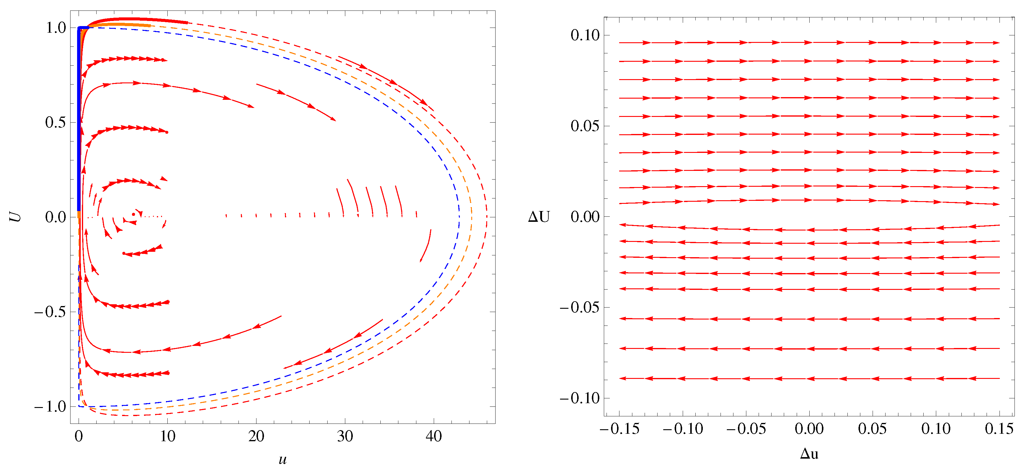
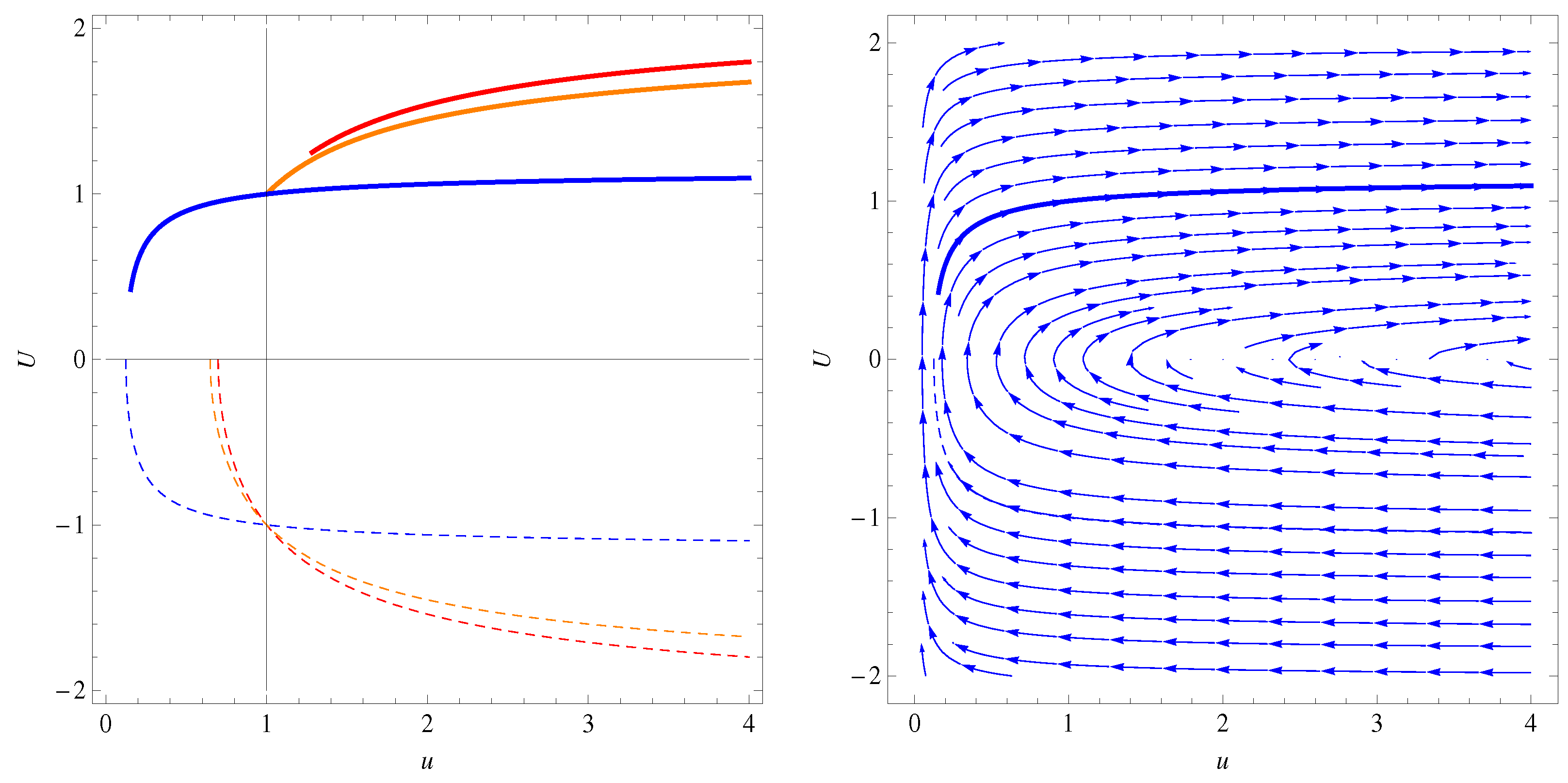
The interdependence between the ion and electron velocities is presented graphically in Figure 5. A key feature to note here, for the nonzero electron mass case, is that the level curves form closed-loops, which confine the fluid velocities to a finite range. The closed-loop curves, of the left hand panel, are plots of as expressed by Equation (82). The three curves plotted correspond to three choices of electron sound speed Mach number: (the unphysical) for the blue curve, for the orange curve and for the red curve. The solid portions of the curves correspond to regions where , as expressed by Equation (81), which we take as a necessary condition for the solution to be physically real. The dashed portions of the curves correspond to (nonphysical) regions where and/or . Overlaid on the curves in the left panel of Figure 5, is the direction field of the solution space for the coupled ODE set (92) displayed as swirling red arrows. This direction field, corresponding to the choice (i.e., the red curve) circles around the stationary point (, ) in a fashion characteristic of harmonic oscillator type ODE systems. To prove that this stationary point is a fixed node, meaning that no solution curves pass through this point, a linear expansion of the ODE set (92) about the stationary point can be effected, which yields pure imaginary eigenvalues of the linearized system; thus the system has a harmonic oscillator character and the fixed point is a node. The direction field corresponding to the linearized ODE system for (92) is presented in the right panel of Figure 5. Evidently, solution curves arbitrarily close to the fixed point (, ) still ‘circle’ around it in oscillator fashion, demonstrating graphically that the fixed point is a node.
In the numerical solutions of the SSS presented, we limit ourselves to a consideration of solutions connected to the NBS. As noted above, if the NBS is chosen as the initial data, the only solution is the constant NBS. To find non-trivial solutions, we look for initial data nearby and connected (via Equations (81) and (82)) to the NBS in the solution space.
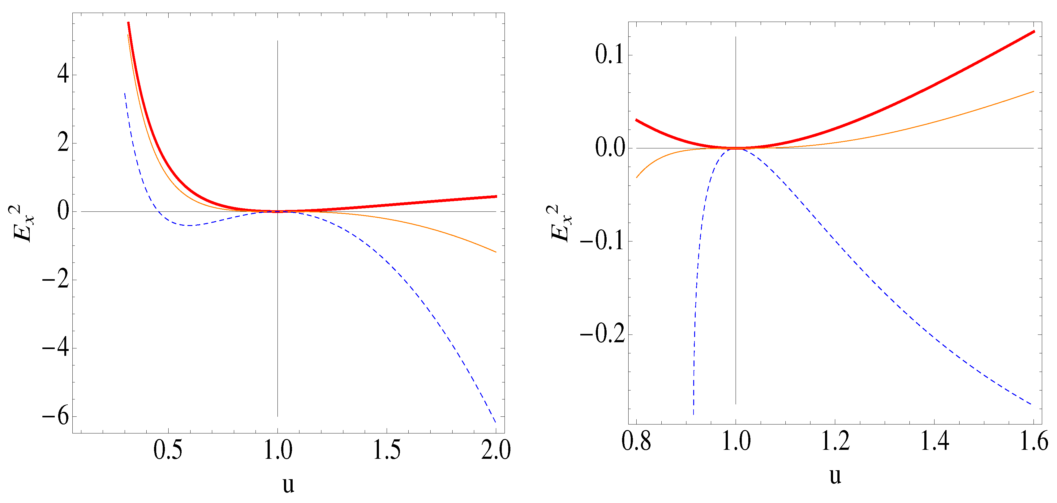
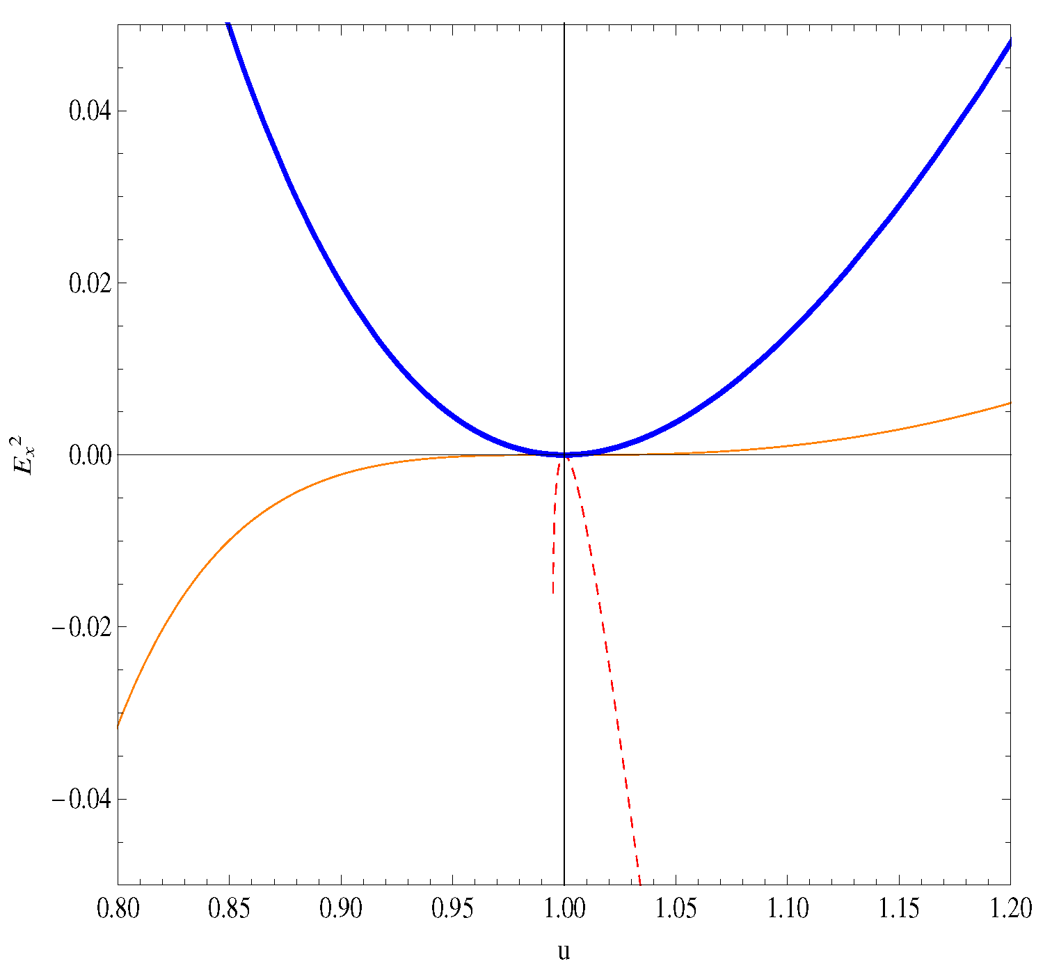
Figure 6 presents plots of curves which simultaneously satisfy both Equation (81) and (82) and helps to illustrate graphically how initial data can be chosen that is near and connected to the NBS in the domain of physically real solutions. The curves of the left panel correspond to (thick red curve), the limiting case (orange curve) and (dashed blue curve). The curves of the right panel correspond to (thick red curve), the limiting case (orange curve) and (dashed blue curve). Assuming that physically real solutions require , then initial data should be chosen from curves that are concave up where they connect to the NBS. Evidently the condition for finding initial conditions associated with physically real solutions is
which is identical to the condition (86) which specifies the region in which the SSS linearized about the NBS posses pure real eigenvalues. In other words if when then the eigenvalues , associated with Equation (83), are real-valued, yielding a linearized solution space characterized by exponential growth. A further implication of the identical conditions (86) and (93) is that the oscillatory (Langmuir wave type) solutions, associated with imaginary , are unobtainable unless we relax the condition that the initial data must be chosen such that solutions pass through the NBS.
We present numerical solutions of the SSS where initial data is chosen such that solution curves are physically connected to the NBS by ensuring that the condition (93) is satisfied. Two distinct classes of solutions (or solution types) become apparent: One type of solution is denoted as an upper solution, meaning that the plasma velocity at the wave center has increased from its initial value. The other solution type presented is denoted as a lower solution, where the plasma velocity decreases from its initial value at the center of the wave.
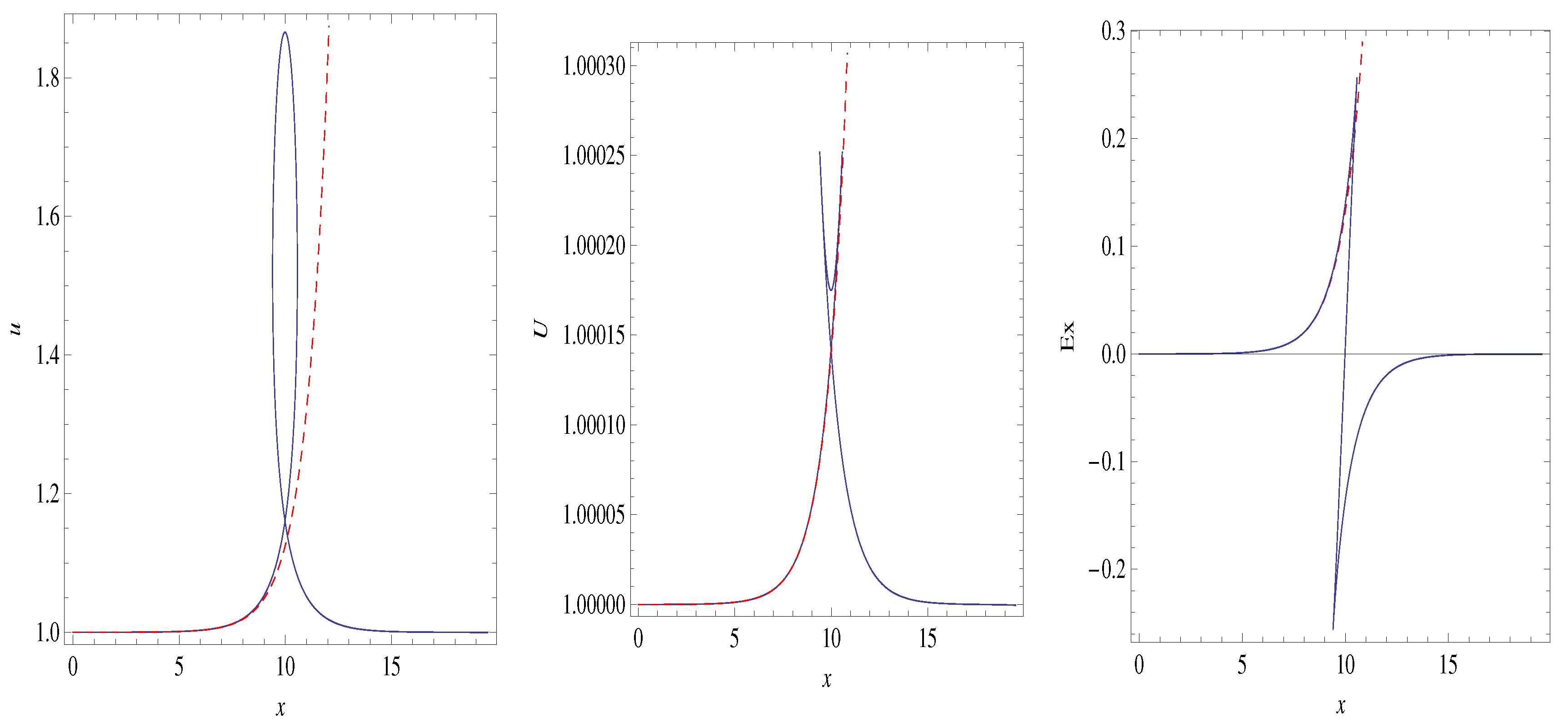
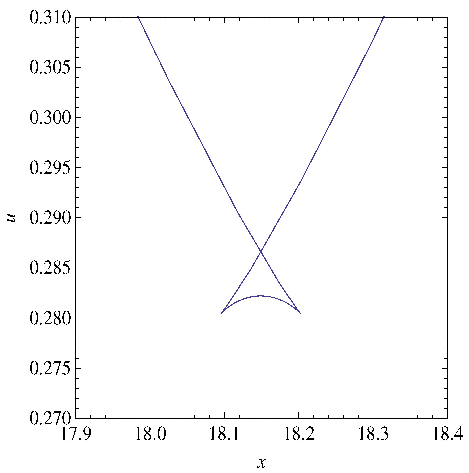
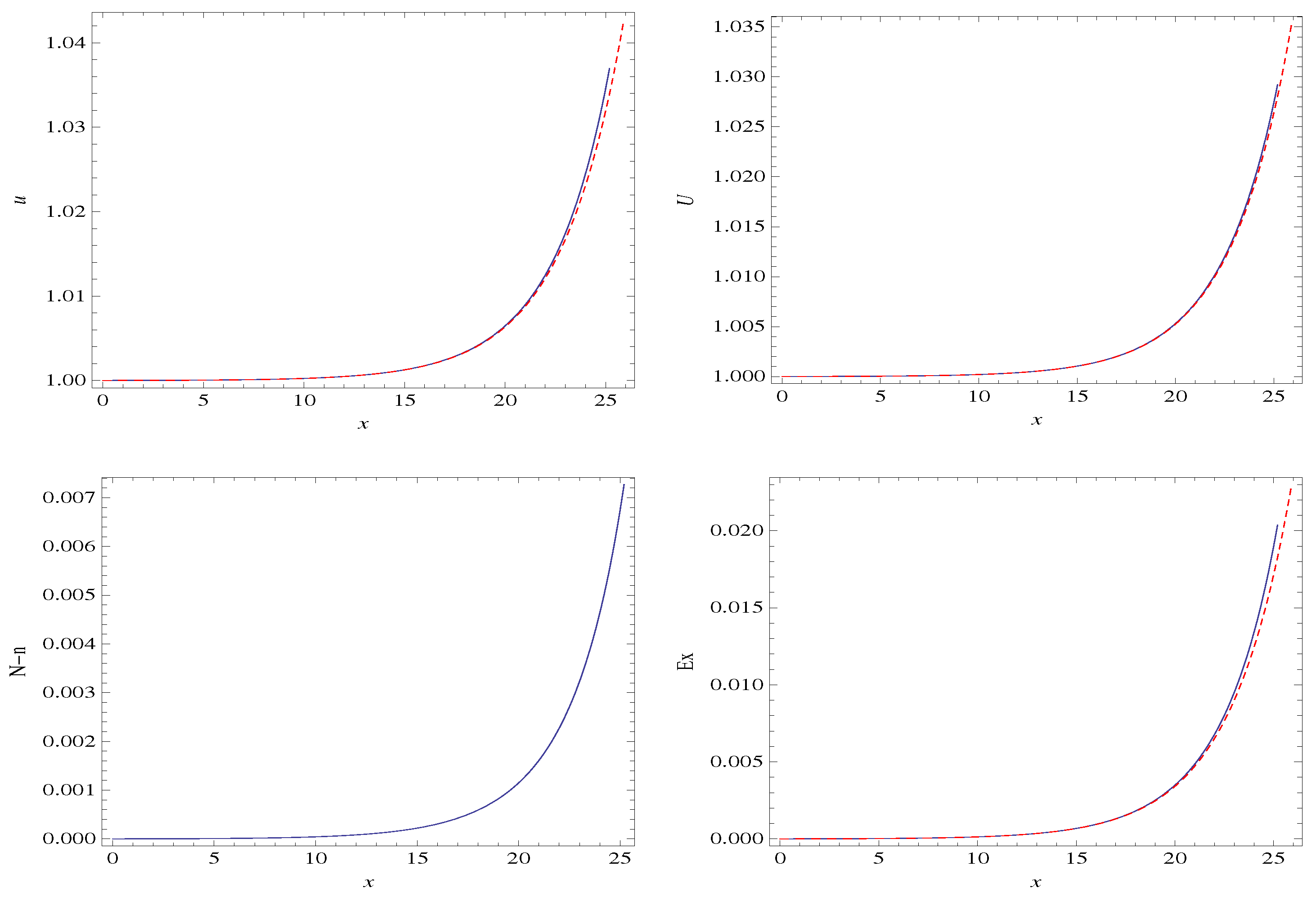
An upper solution of the SSS Equations (87) through (90), for the choice , is plotted in Figure 7. The solid blue curves are parametric plots of the form . The dashed red curves are plots of the corresponding solution (84), , of the linearized SSS (83). As evidenced by inspection of Figure 7, the state variables , for the nonlinear case, are double valued in the region on the x-axis sandwiched between the sonic points where and (see Equation (78)). A natural question to ask is can a unique, single-valued solution be constructed from the double-valued parametric solution?
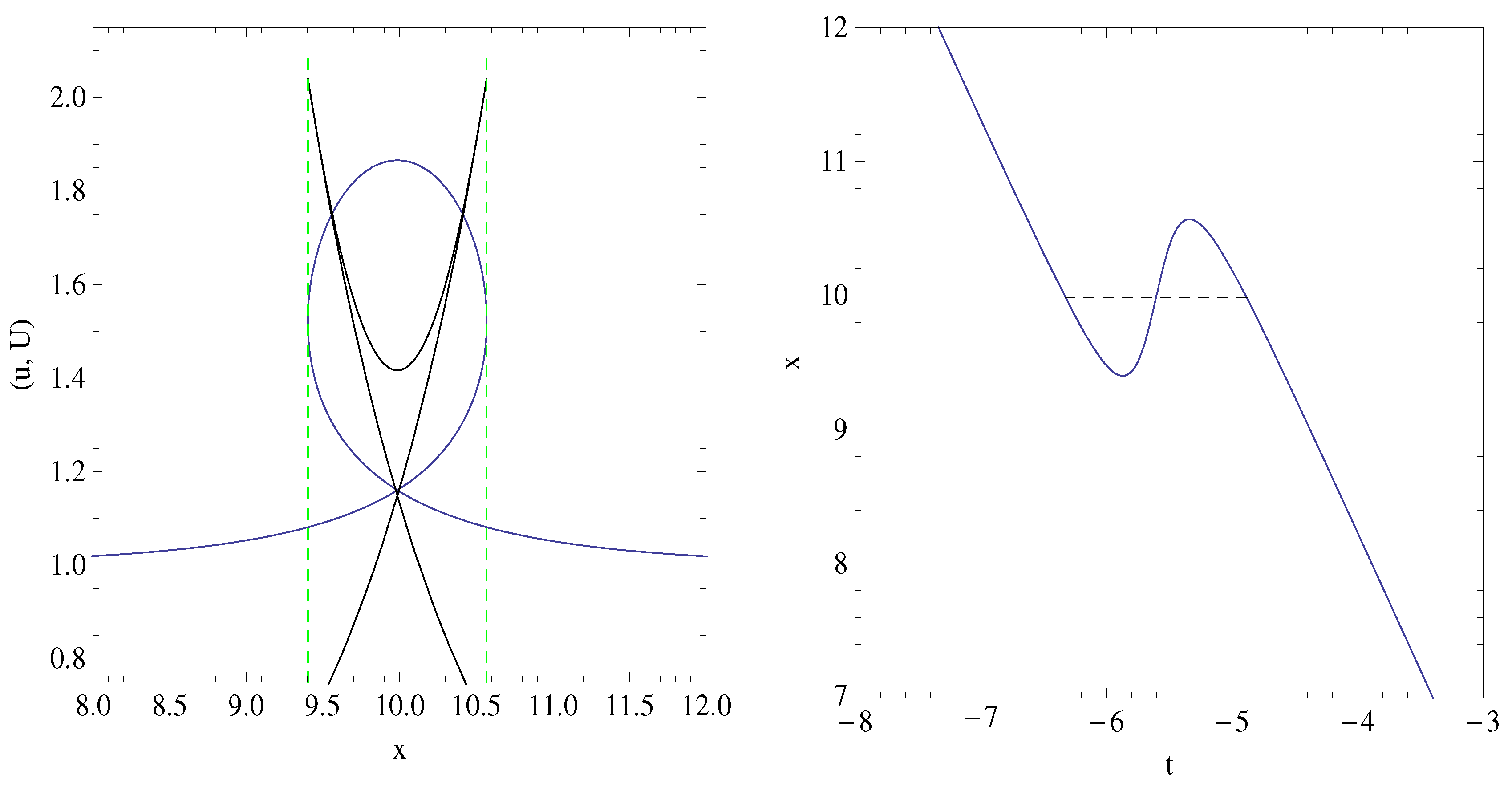
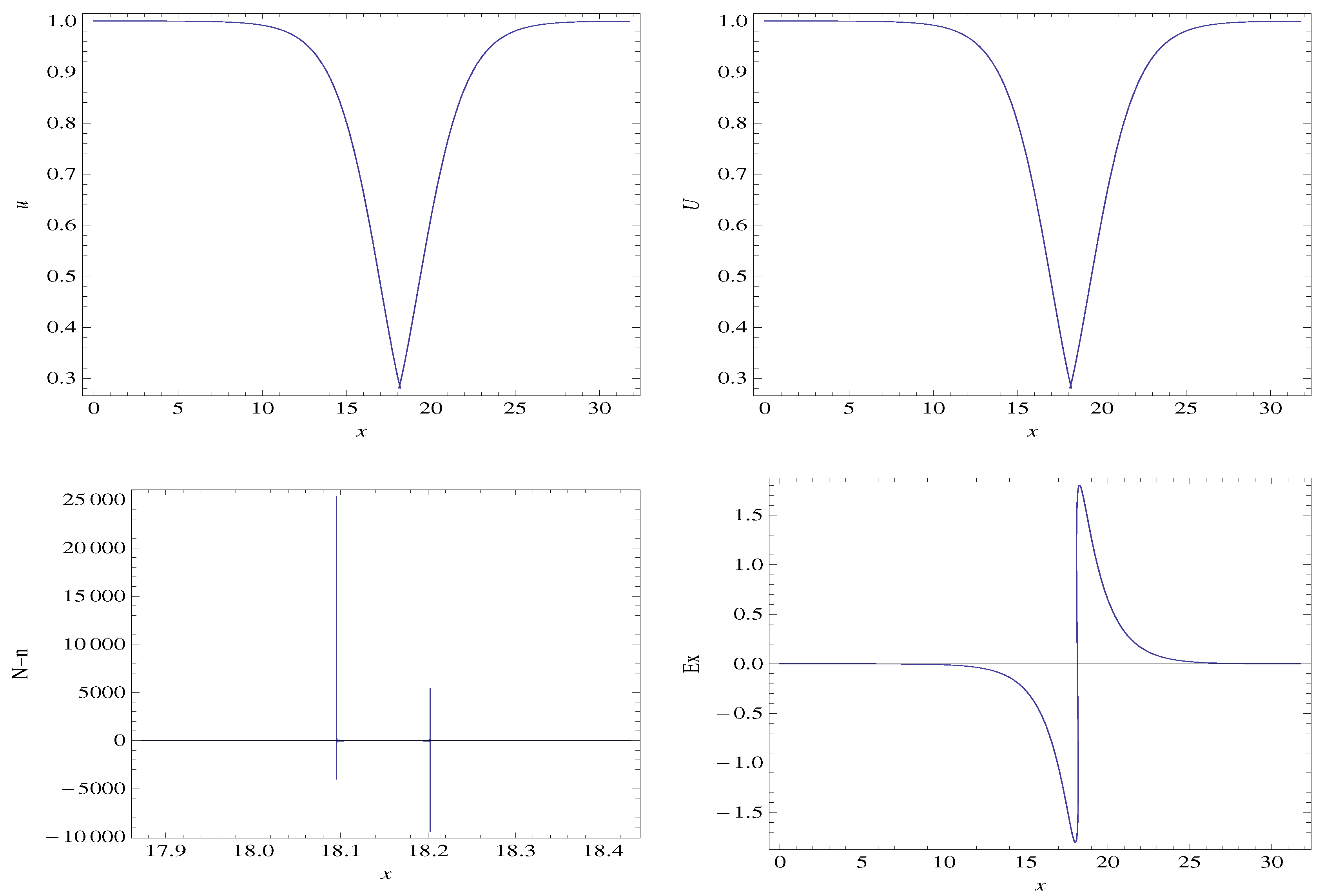
Inspection of Figure 8 indicates how a unique solution can be constructed from the double valued parametric solution. The left panel of the figure shows the solution curve for (blue curve) plotted on the same axis with (black curve—nonphysically scaled-up for visual clarity). The vertical, dashed, green lines are tangent to the u-curve at the sonic points where and . As required by Equation (82) (and illustrated graphically in Figure 5), the sonic points are also locations where must reach a maximum. Note that at the bisector between the sonic points the slopes and , which, by inspection of the SSS, requires that at the bisector also. The value of at the bisector (or wave center) can found from the plot of (blue curve) shown in the right panel of Figure 5. This plot shows that x is everywhere increasing with decreasing parameterization variable t, except in the region near the sonic points, where is double valued. To construct the unique solution, note that a horizontal line drawn between the two sonic points (dashed, black, horizontal line of the right panel) separates the double valued regions into two lobes of equal area. This suggests that (analogous to Van der Waals isothermal construction) a single-valued solution can be formed by removing the lobes and joining the curve along the horizontal, dashed, line segment. This equal area construction requires that the line segment be inserted precisely at the bisector value of , directly in the center of the symmetrical wave structure and effectively ‘scissor-cuts’ the top, double-valued lobes off of the u and U curves and joins the lower parts of the curves together with an infinitesimally narrow horizontal line along which the slopes and . This solution is unique since there is only one point on the x-axis where the segment is inserted such that it is entirely compatible with the original SSS equations. Note that at the point where the horizontal segment is inserted the charge density of the plasma behaves like a delta function since .
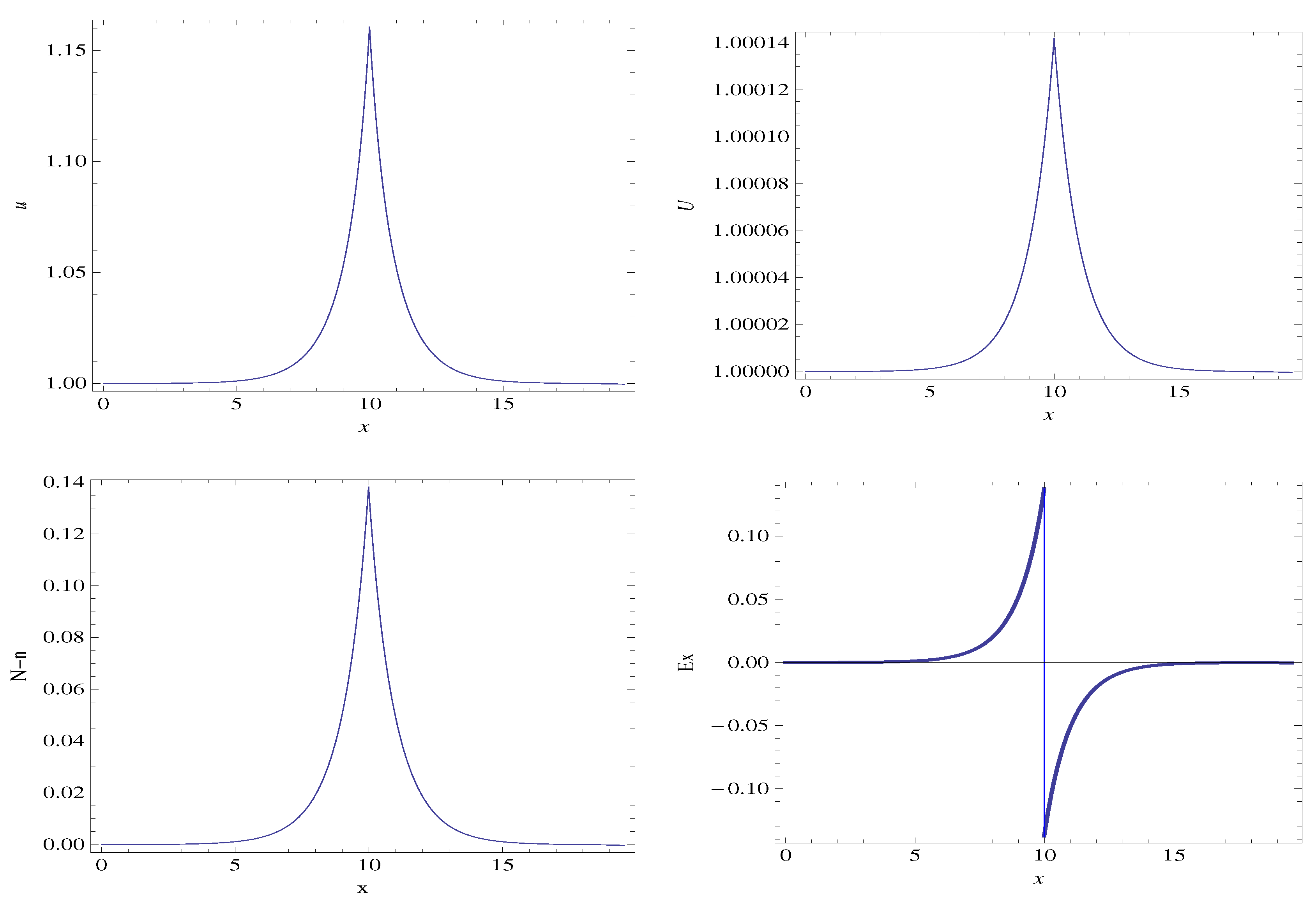
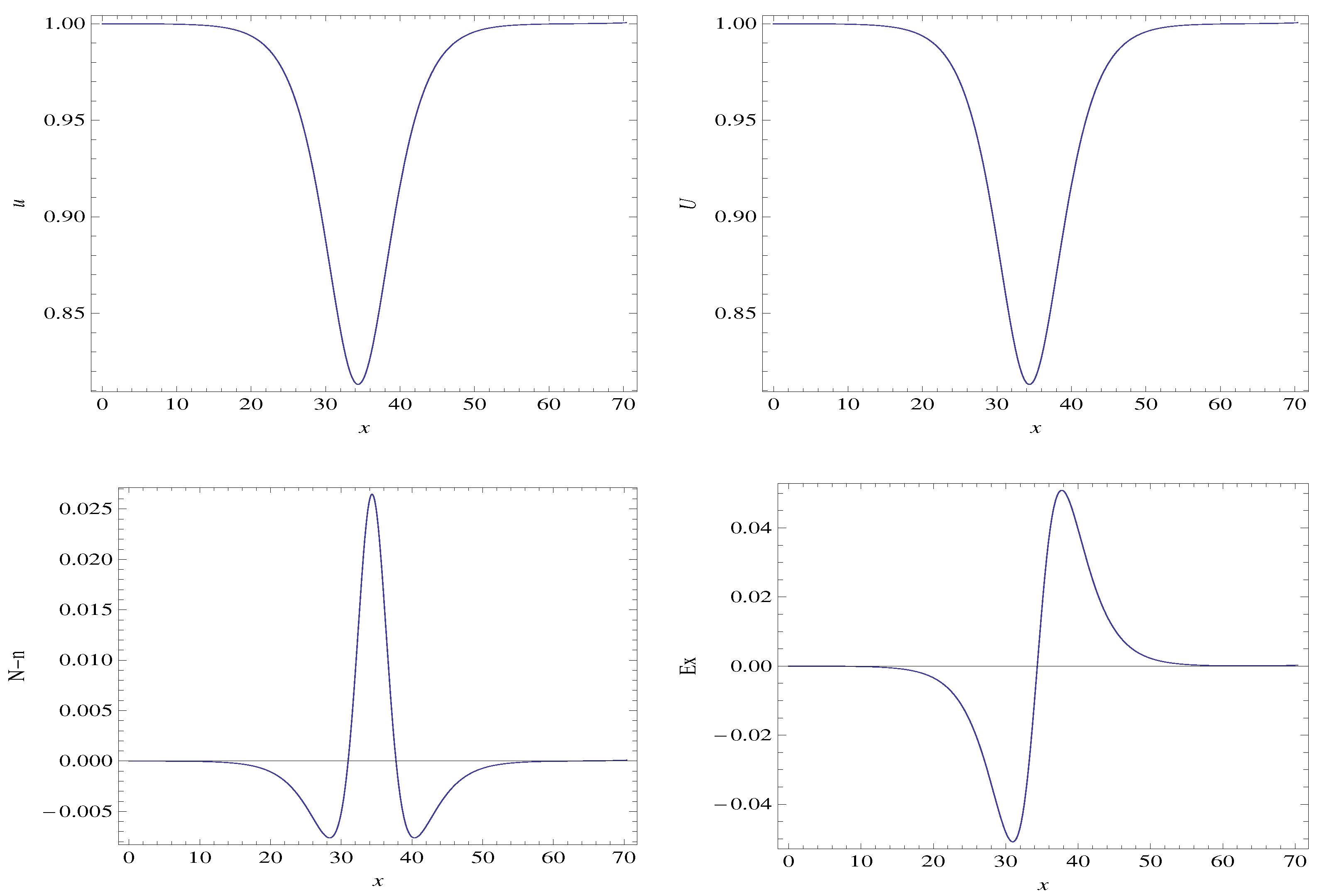
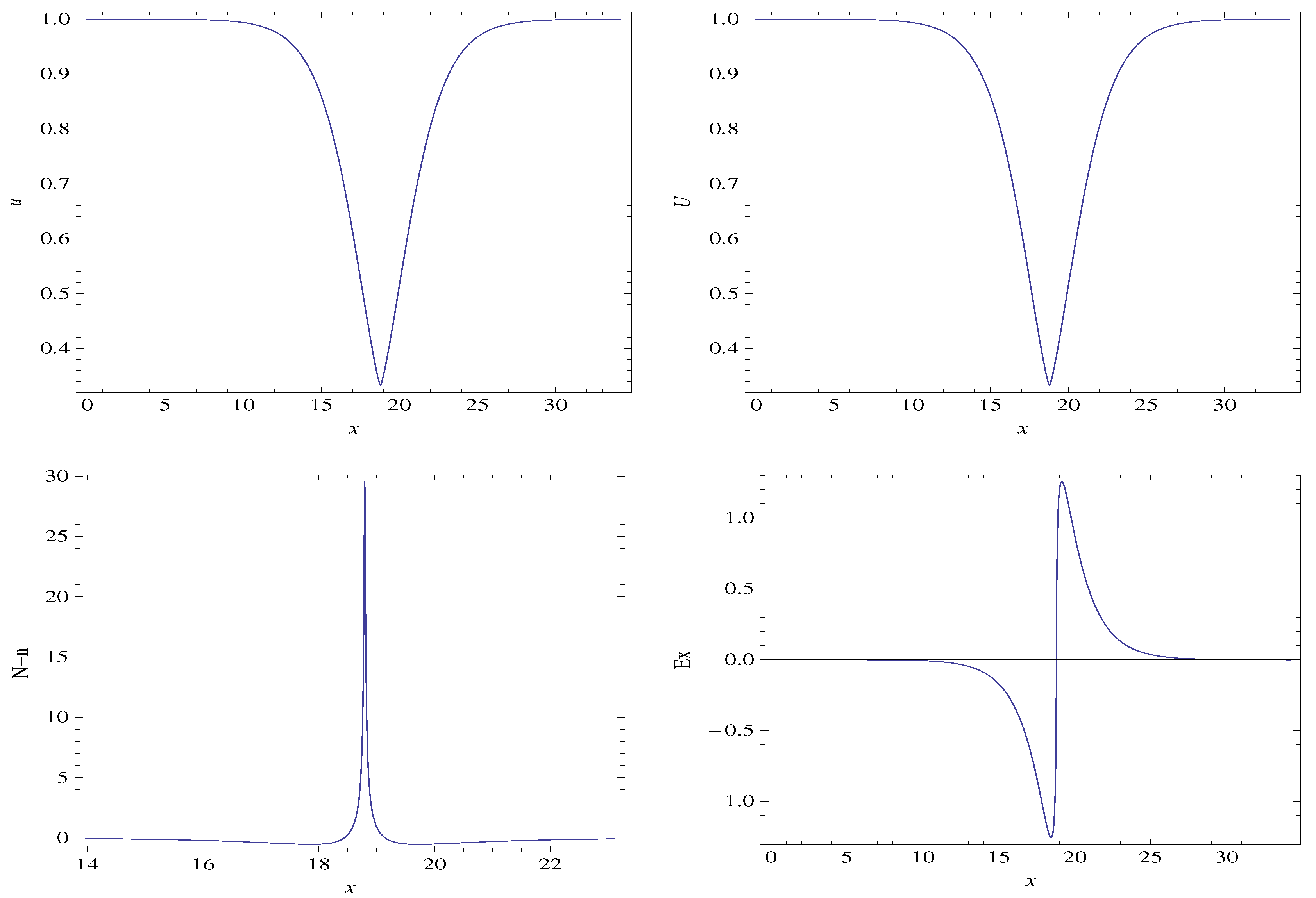
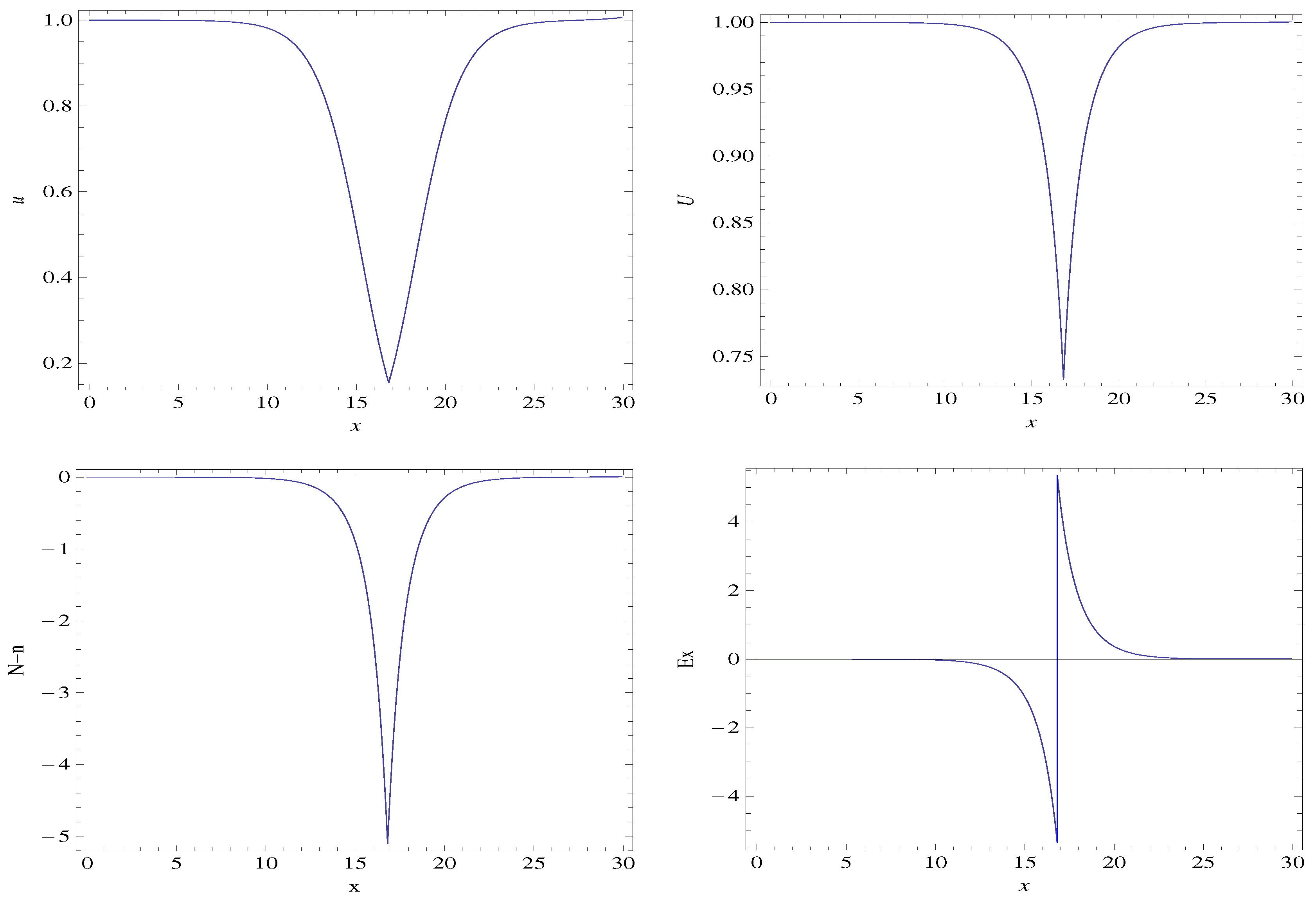
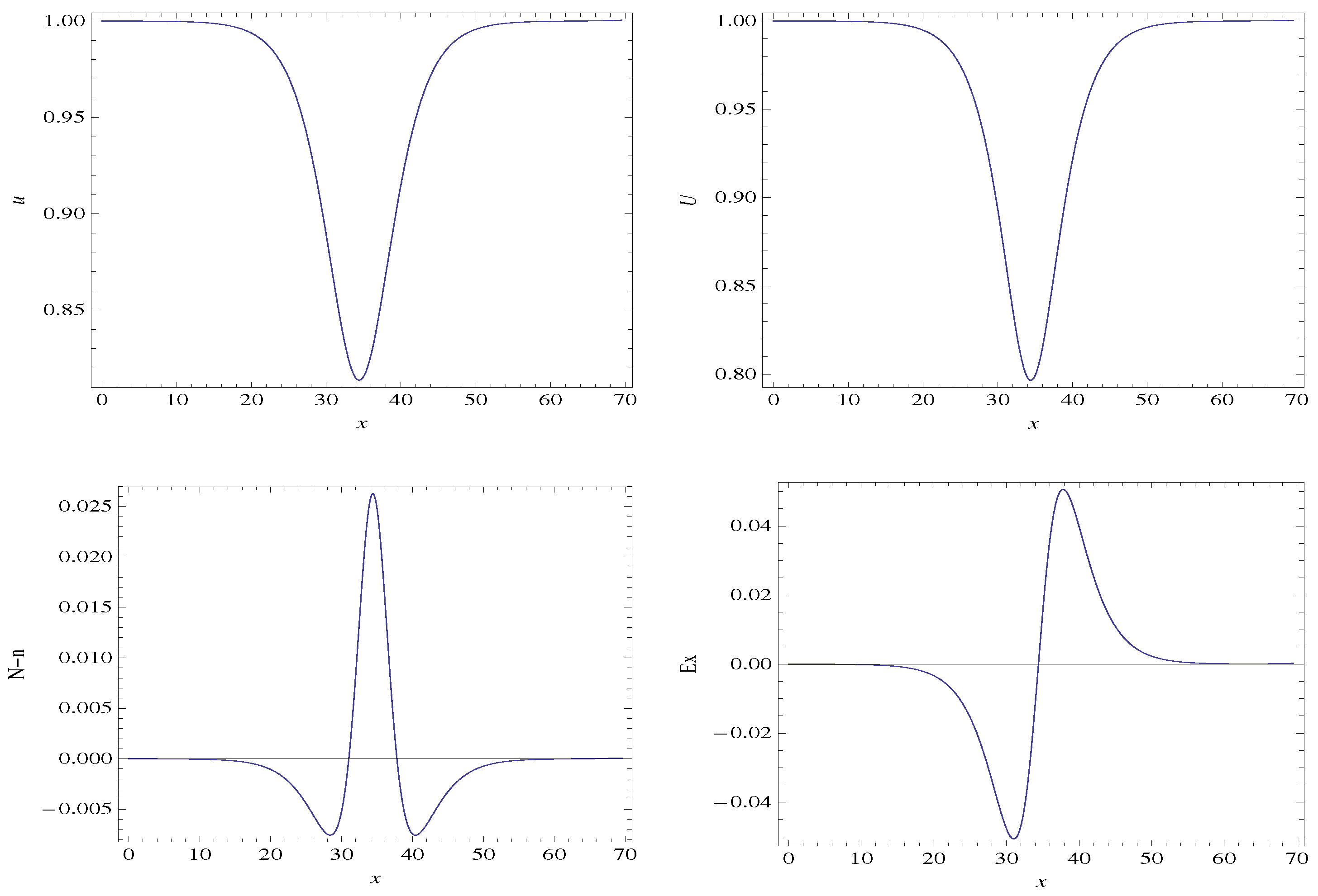
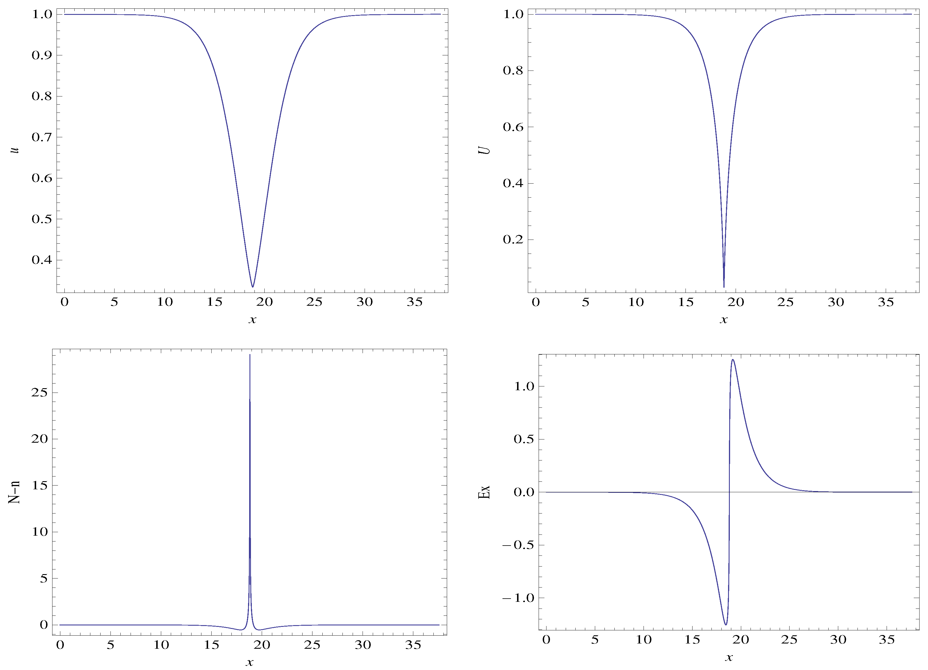
The sharply peaked upper solution for the choice , is presented in Figure 9. In terms of the collective Mach number
this choice corresponds to . The electron velocity (top left panel), evidently possesses a substantially stronger amplitude then the ion velocity (top right panel). The density difference (governing Possion’s equation), plotted in the lower left panel, reaches a maximum of ∼14% also at the sonic point bisector; however note that the insertion of the unique solution implicitly requires that be a delta type function at , but this behavior has not been included in the plot. The single valued solution for (lower right panel) is constructed by joining the positive and negative solution branches with a vertical line inserted at the sonic point bisector, where it is implied that , and removing the double valued curve portions that extend beyond this line. The construction of the single valued solution highlights the importance of the sonic point , the existence of which implies a location : the point where flow-rate that would otherwise be growing exponentially gets choked off and forced to decelerate back to the NBS.
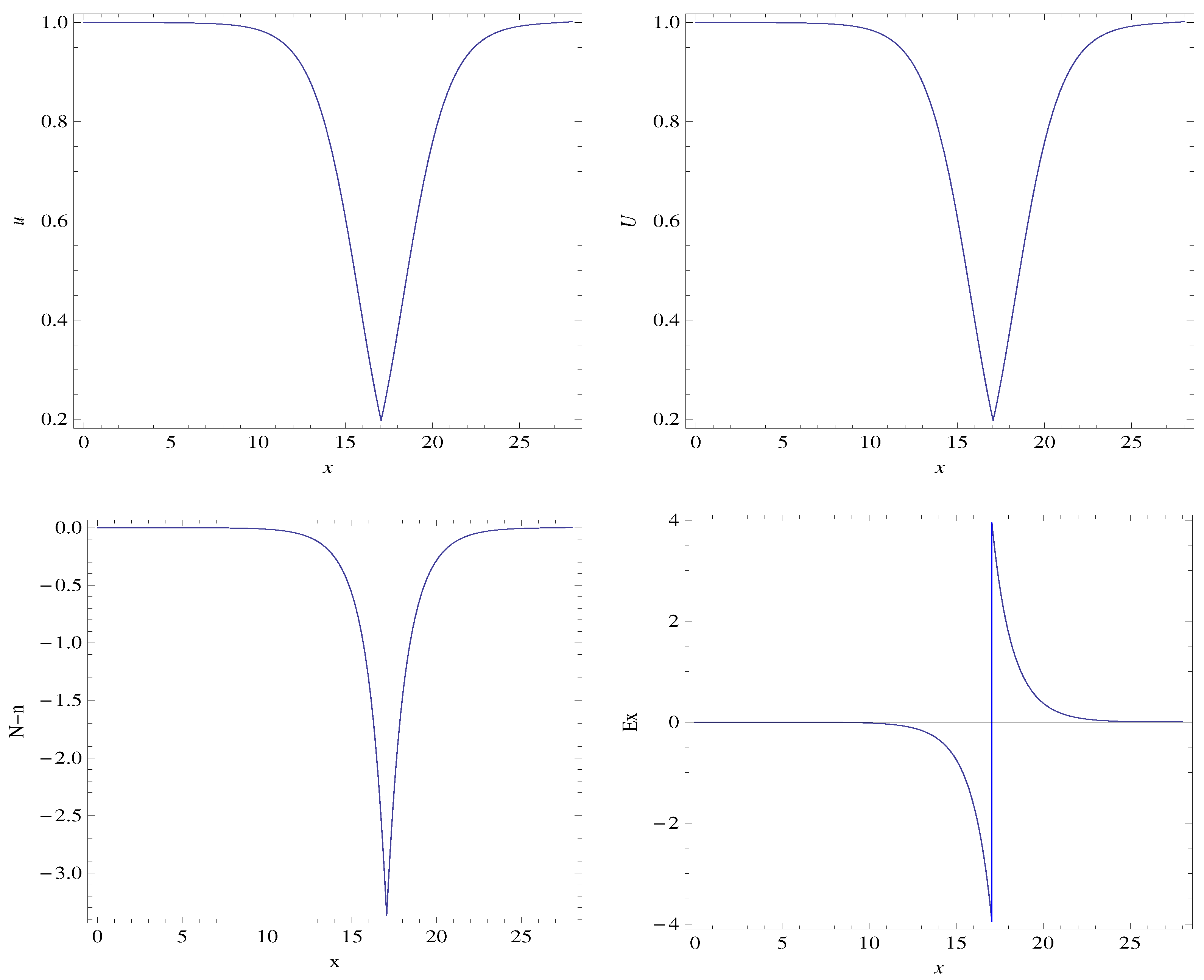
Lower solutions are presented in Figure 10, Figure 11, Figure 12, Figure 13 and Figure 14. For lower values of the collective ion-acoustic Mach number (e.g., ) these solution curves are smooth, single valued and do not require the insertion of a unique solution.
For the choice and higher, the decelerating solutions become double valued near the wave center consistent with the findings of McKenzie (2002) [29]). Figure 13, corresponding to , shows a close-up view of near the wave center, revealing the double valued character of the solution. In these double valued, decelerating cases, a unique solution can be inserted using the method described above, in which the value of at the wave center is found from an equal area construction (see Figure 8).
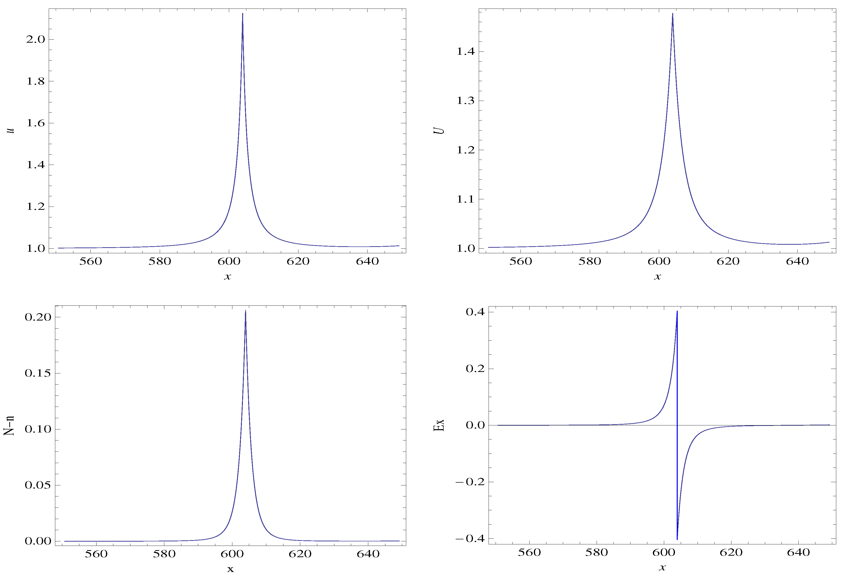
Figure 14, for illustrates a lower solution constructed in the same manner as described above for upper solutions. Some general trends that can be noted about such decelerating solutions are that the wave amplitude increases linearly with increasing Mach number, going from roughly for to for . On the other hand, the wave structure narrows with increasing Mach number, going from about 400 Debye lengths when and narrowing down to about 15 Debye lengths at after which the wave structure tends towards a constant minimum in that there is no further width decrease for increasing Mach number.
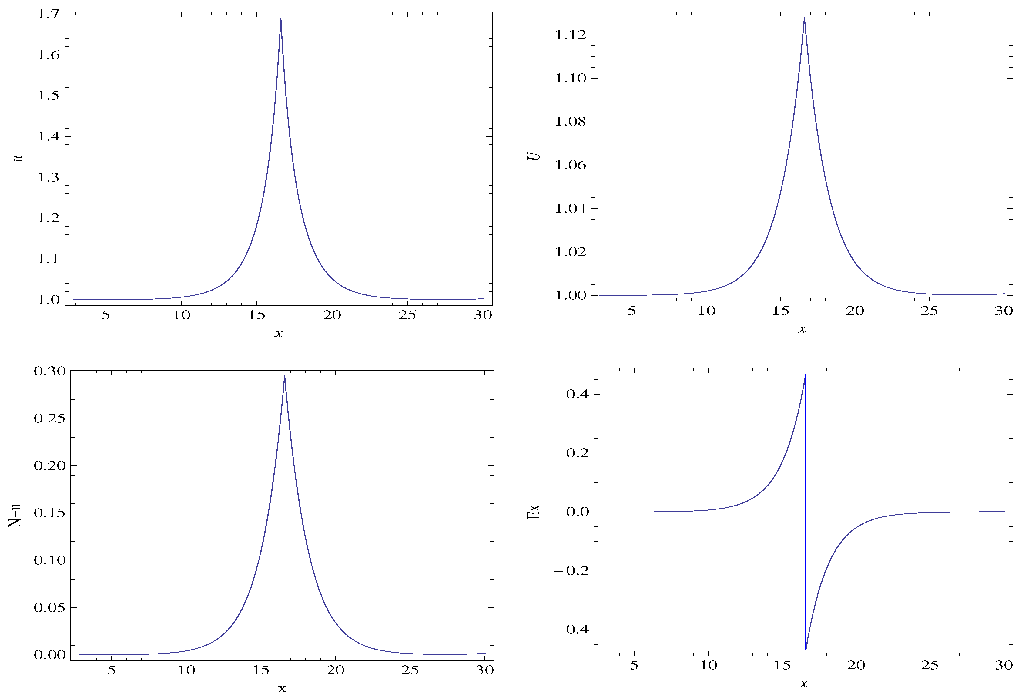
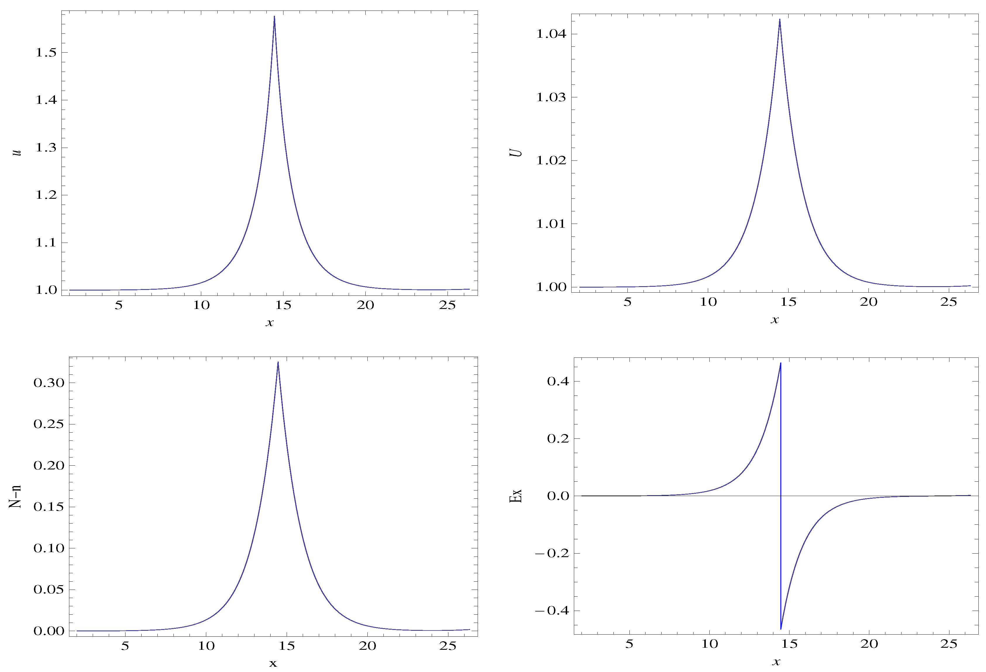
Upper solutions for Mach numbers 1, 1.8 and 3, constructed using the procedure described above, are presented in Figure 15, Figure 16 and Figure 17. The upper solutions also become increasingly narrow with increasing Mach number, going from a width of roughly 40 Debye lengths when down to about 15 Debye lengths when and then remaining roughly constant at this value for increasing Mach number. The amplitude of accelerating (weak) solutions is, evidently, highly insensitive to Mach number variation, going from when and remaining at for Mach numbers of and higher.
3.2. Setting the Electron Mass to Zero
To understand the significance of electron mass in the SSS, we can consider the limit , which effectively removes the electron-acoustic, sonic point from the system. The zero electron mass form of the SSS can readily be obtained by keeping only terms with a factor in the momentum equations and by dropping all terms with an factor from the conservation equations. This yields the governing system of ODEs
which contain the integrals
and
where the parameter is here most conveniently expressed in terms of the ‘collective ion-acoustic Mach number’ [29]
as
The SSS (94) through (96) again is stationary at the NBS.
The SSS for , linearized about the NBS, is
As with the previous case, the solution of Equation (99) has the general form (84) and also possesses the eigenvalue with the associated eigenvector , with the implication that the NBS as a constant state is built into the system. The remaining two eigenvalues for (99) can be expressed as
thus, the eigenvalues will be pure real whenever
and pure imaginary otherwise. With , Equations (91) and (92) become
and
Comparison of these analogous figures shows that a key difference between the zero and nonzero electron mass cases is that when the sonic point is effectively shifted to infinity on the u-axis. Thus, the proton verses electron velocity dependence, which is characterized by closed-loop (oscillator type) curves in phase-space for nonzero electron mass, becomes an open (on the right), unbounded electron velocity curve when .
Figure 18 and Figure 19 express, graphically, the condition required for solutions to connectable physically to the NBS.
Figure 20 is the only upper-solution presented for . As noted above, setting the electron mass to zero has effectively shifted the sonic point to infinity, meaning that the upward growing electron velocity is unbounded and thus unphysical in this case.
3.3. Discussion
While the treatment of the two-fluid system, considered here above, is simply a variation on the gas dynamic descriptions of ESWs presented by e.g., McKenzie and Verheest [7,30], it does have the advantage of yielding two types of ESW structures, via slight perturbations on the same background plasma conditions, for which the previously mentioned analytic methods would yield only a single ESW wave structure. Indeed, the classic Sagdeev potential method [31], and the more modern gas-dynamic view-points [7,30,32] derived from it, offer very attractive, analytic descriptions of ESWs. These analytic approaches [7,30], well define the exact conditions for which smooth ESW solutions can be constructed. The interesting feature of the (essentially numeric, gas dynamic) treatment considered here, however, is that we show how an additional non-smooth, or shock-like, ESW can also be constructed by the explicit insertion of a jump through the charge neutral point of the wave. This extra jump solution (denoted here as an accelerating upper solution in the text) is associated with negative potential wells, whereas the smooth solution that would naturally arise using more analytic methods (denoted here as a decelerating lower solution in the text) is associated with positive potential hills (e.g., see [33].) As suggested above, the proximate excitation of both upper and lower ESWs, by small perturbations from the same plasma background conditions, may be supported by observations.
4. Conclusions
The need for a self consistent system of multi-fluid equations which dynamically includes a small population of hot, energetic particles, such as pickup ions (treated kinetically as is done in PIC codes) has been addressed. We previously presented a multi-fluid treatment which included a population of kinetically treated pickup ions (PUIs) coupled to a two-fluid treatment with quasi self-consistent coupling through the anisotropic PUI pressure tensor [6]. Here we considered an improvement of that model with a small population of kinetic ions included in the multi-fluid system by a self-consistent treatment of their charge density and current component effects on the electromagnetic fields.
By considering the reduction of the multi-fluid plasma system to the special case of hot electrons and cold ions in the steady state, the existence of two types of electrostatic solitary waves (ESWs) were shown, characterized and typed here as upper and lower solutions. The character of the upper and lower solutions of the coupled set of ODEs are consistent with the two types of ESWs observed by Geotail near Earth’s bow shock [11], with one type of ESW associated with electrostatic potential hills and the other with potential wells.
We have shown that setting (a typical approximation for PIC as well as other simulations) recovers classical solitons, labeled here as lower solutions, such as presented in the well known text book on plasma physics by Chen [31].
A type of soliton, labeled as upper solutions, was found that depends critically on a nonzero electron mass to prevent unbounded acceleration of the electron fluid velocity. These so-called upper solutions are consistent with the second type of ESW observed by Geotail [11] associated with ‘positive’ electrostatic potential hills and components of two-fluid plasma flow returning upstream from the ESWs towards the bow shock.
The width of upper solutions were found to decrease with increasing Mach number, asymptotically reaching a minimum width of about 15 Debye lengths at . The amplitude of upper solutions is highly insensitive to Mach number and have a magnitude of the electric field of (in normalized units) for all Mach numbers. Upper solutions also become more narrow with increasing Mach number, asymptotically reaching a minimum scale width of roughly 15 Debye lengths.
The classical type solitons, or lower solutions, were found to have an electric field strengths that grow linearly with increasing Mach number. Lower solutions are smooth functions and straight-forward to evaluate over the Mach number range (for ). However for all upper solutions and for lower solutions where , the insertion of a unique solution is required.
A method for constructing unique solutions was outlined, and applied to both upper and lower types, where at the insertion point on the x-axis, the charge density is viewed as a delta like function where and the electric field is forced to zero by insertion of a unique solution, with the result that a bounded, single-valued solution is formed that is fully compatible with the original governing system of ODEs.
Funding
This research received no external funding.
Conflicts of Interest
The author declares no conflict of interest.
Abbreviations
The following abbreviations are used in this manuscript:
| MDPI | Multidisciplinary Digital Publishing Institute |
| DOAJ | Directory of open access journals |
| MRI | multiply reflected ion |
| PUI | pickup ion |
| SW | solar wind |
| PIC | particle-in-cell |
| MHD | magnetohydrodynamics |
| ESW | electrostatic solitary wave |
| ODE | ordinary differential equation |
| SDA | shock drift acceleration |
| SSA | shock surfing acceleration |
| TS | Termination Shock |
| CSP | cross-shock potential |
| SAP | shock accelerated particle |
| B&S | Boyd and Sanderson |
| AU | astronomical unit |
| 1D | one dimensional |
| SS | steady state |
| NBS | neutral background state |
| SSS | steady state system |
References
- Burrows, R.H.; Zank, G.P.; Webb, G.M.; Burlaga, L.F.; Ness, N.F. Pickup Ion Dynamics at the Heliospheric Termination Shock Observed by Voyager 2. Astrophys. J. 2010, 715, 1109–1116. [Google Scholar] [CrossRef]
- Zank, G.P.; Pauls, H.L.; Cairns, I.H.; Webb, G.M. Interstellar pickup ions and quasi-perpendicular shocks: Implications for the termination shock and interplanetary shocks. J. Geophys. Res. 1996, 101, 457–478. [Google Scholar] [CrossRef]
- Lee, M.A.; Shapiro, V.D.; Sagdeev, R.Z. Pickup ion energization by shock surfing. J. Geophys. Res. 1996, 101, 4777–4790. [Google Scholar] [CrossRef]
- Zank, G.P.; Heerikhuisen, J.; Pogorelov, N.V.; Burrows, R.; McComas, D. Microstructure of the Heliospheric Termination Shock: Implications for Energetic Neutral Atom Observations. Astrophys. J. 2010, 708, 1092–1106. [Google Scholar] [CrossRef]
- Zank, G.P.; Burrows, R.; Oka, M.; Dasgupta, B.; Heerikhuisen, J.; Webb, G.M. Micro-Structure of the Heliospheric Termination Shock. In Proceedings of the 8th Annual International Astrophysics Conference, Kona, HI, USA, 1–7 May 2009; Ao, X., Burrows, G.Z.R., Eds.; American Institute of Physics: College Park, MD, USA, 2009; Volume 1183, pp. 156–166. [Google Scholar] [CrossRef]
- Burrows, R.H.; Ao, X.; Zank, G.P. A New Hybrid Method. In Outstanding Problems in Heliophysics: From Coronal Heating to the Edge of the Heliosphere; Hu, Q., Zank, G.P., Eds.; ASP: San Francisco, CA, USA, 2014; Volume 484. [Google Scholar]
- McKenzie, J.F. Electron acoustic-Langmuir solitons in a two-component electron plasma. J. Plasma Phys. 2003, 69, 199–210. [Google Scholar] [CrossRef]
- Burrows, R.H.; Ao, X.; Zank, G.P. Shock Surfing at a Two-Fluid Plasma Model; American Institute of Physics Conference Series; American Institute of Physics: College Park, MD, USA, 2012. [Google Scholar]
- Richardson, J.D.; Kasper, J.C.; Wang, C.; Belcher, J.W.; Lazarus, A.J. Cool heliosheath plasma and deceleration of the upstream solar wind at the termination shock. Nature 2008, 454, 63–66. [Google Scholar] [CrossRef]
- Oka, M.; Zank, G.P.; Burrows, R.H.; Shinohara, I. Energy Dissipation at the Termination Shock: 1D PIC Simulation. In Proceedings of the 2010 Huntsville Workshop, Nashville, TN, USA, 3–8 October 2010; American Institute of Physics Conference Series. Florinski, V., Heerikhuisen, J., Zank, G.P., Gallagher, D.L., Eds.; American Institute of Physics: College Park, MD, USA, 2011; Volume 1366, pp. 53–59. [Google Scholar] [CrossRef]
- Shin, K.; Kojima, H.; Matsumoto, H.; Mukai, T. Characteristics of electrostatic solitary waves in the Earth’s foreshock region: Geotail observations. J. Geophys. Res. 2008, 113, A03101. [Google Scholar] [CrossRef]
- Wilson, L.B., III; Cattell, C.; Kellogg, P.J.; Goetz, K.; Kersten, K.; Hanson, L.; MacGregor, R.; Kasper, J.C. Waves in Interplanetary Shocks: A Wind/WAVES Study. Phys. Rev. Lett. 2007, 99, 041101. [Google Scholar] [CrossRef] [Green Version]
- Bale, S.D.; Kellogg, P.J.; Larson, D.E.; Lin, R.P.; Goetz, K.; Lepping, R.P. Bipolar electrostatic structures in the shock transition region: Evidence of electron phase space holes. Geophys. Res. Lett. 1998, 25, 2929–2932. [Google Scholar] [CrossRef]
- Tidman, D.A.; Krall, N.A. Shock Waves in Collisionless Plasmas; Wiley Series in Plasma Physics; Wiley-Interscience: New York, NY, USA, 1971. [Google Scholar]
- Noguchi, K.; Tronci, C.; Zuccaro, G.; Lapenta, G. Formulation of the relativistic moment implicit particle-in-cell method. Phys. Plasmas 2007, 14, 042308. [Google Scholar] [CrossRef] [Green Version]
- Lapenta, G. Particle simulations of space weather. J. Comput. Phys. 2012, 231, 795–821. [Google Scholar] [CrossRef]
- Hoshino, M. Coupling Across Many Scales. Science 2003, 299, 834–835. [Google Scholar] [CrossRef] [PubMed]
- Webb, G.M.; Axford, W.I.; Terasawa, T. On the drift mechanism for energetic charged particles at shocks. Astrophys. J. 1983, 270, 537–553. [Google Scholar] [CrossRef]
- Pogorelov, N.V.; Zank, G.P.; Ogino, T. Three-dimensional Features of the Outer Heliosphere due to Coupling between the Interstellar and Interplanetary Magnetic Fields. II. The Presence of Neutral Hydrogen Atoms. Astrophys. J. 2006, 644, 1299–1316. [Google Scholar] [CrossRef]
- Winske, D.; Daughton, W. Generation of lower hybrid and whistler waves by an ion velocity ring distribution. Phys. Plasmas 2012, 19, 072109. [Google Scholar] [CrossRef] [Green Version]
- Boyd, T.M.M.; Sanderson, J.J. Plasma Dynamics; Barnes & Nobel, Inc.: New York, NY, USA, 1969. [Google Scholar]
- Zank, G.P. Interaction of the solar wind with the local interstellar medium: A theoretical perspective. Space Sci. Rev. 1999, 89, 413–688. [Google Scholar] [CrossRef]
- Dudík, J.; Dzifčáková, E.; Meyer-Vernet, N.; Del Zanna, G.; Young, P.R.; Giunta, A.; Sylwester, B.; Sylwester, J.; Oka, M.; Mason, H.E.; et al. Nonequilibrium Processes in the Solar Corona, Transition Region, Flares, and Solar Wind (Invited Review). Sol. Phys. 2017, 292, 100. [Google Scholar] [CrossRef]
- Yoon, P.H. Electron kappa distribution and quasi-thermal noise. J. Geophys. Res. 2014, 119, 7074–7087. [Google Scholar] [CrossRef]
- Livadiotis, G.; McComas, D.J. Understanding Kappa Distributions: A Toolbox for Space Science and Astrophysics. Space Sci. Rev. 2013, 175, 183–214. [Google Scholar] [CrossRef] [Green Version]
- McComas, D.J.; Allegrini, F.; Bochsler, P.; Bzowski, M.; Christian, E.R.; Crew, G.B.; DeMajistre, R.; Fahr, H.; Fichtner, H.; Frisch, P.C.; et al. Global Observations of the Interstellar Interaction from the Interstellar Boundary Explorer (IBEX). Science 2009, 326, 959. [Google Scholar] [CrossRef]
- Ao, X.; Burrows, R.H.; Zank, G.P.; Webb, G.M. Solitons in two-fluid plasma. In Proceedings of the 10th Annual International Astrophysics, Maui, HI, USA, 13–18 March 2011; Heerikhuisen, J., Li, G., Pogorelov, N., Zank, G., Eds.; American Institute of Physics: College Park, MD, USA, 2011; Volume 1436, pp. 5–11. [Google Scholar]
- Zank, G.P.; McKenzie, J.F. Solitons in an ion-beam plasma. J. Plasma Phys. 1988, 39, 183–191. [Google Scholar] [CrossRef]
- McKenzie, J.F. The ion-acoustic soliton: A gas-dynamic viewpoint. Phys. Plasmas 2002, 9, 800–805. [Google Scholar] [CrossRef]
- Verheest, F.; Cattaert, T.; Lakhina, G.S.; Singh, S.V. Gas-dynamic description of electrostatic solitons. J. Plasma Phys. 2004, 70, 237–250. [Google Scholar] [CrossRef]
- Chen, F.F. Introduction to Plasma Physics and Controlled Fusion; Plenum Press: New York, NY, USA, 1984. [Google Scholar]
- Verheest, F.; Hellberg, M. Electrostatic solitons and sagdeev psuedopentials in space plasmas: Review of recent advances. In Handbook of Solitons; Nova Science Publishers: New York, NY, USA, 2009; pp. 353–393. [Google Scholar]
- Webb, G.M.; Burrows, R.H.; Ao, X.; Zank, G.P. Ion acoustic traveling waves. J. Plasma Phys. 2014, 80, 147–171. [Google Scholar] [CrossRef] [Green Version]
Figure 1.
Illustration of the idealized initial ion distribution, in the shock frame, before and just after reflection. (a) The unreflected initial distribution is composed of a pickup ions (PUIs) which reside on a shell in velocity space of radius (the solar wind (SW) speed) and SW ions residing in a core located at (). The dashed portion of the PI shell to the left of on the -axes (vertical dashed line) has an insufficient x-component of velocity to over come the cross-shock potential (CSP, ) and will be reflected. (b) The ion distribution immediately following refection is composed of the specularly reflected fractional part of the PUI shell and the remainder which, along with the SW core, is convected downstream without reflection. Not illustrated by this figure is the stretching along motional electric field () direction that the reflected partial shell will undergo during the energization process. It is evident that the reflected PUI partial shell has gained energy after a single reflection, with respect to the fluid frame where the SW core is at the origin.

Figure 2.
A test-particle ion (lower black curve) shock surfing through a model of the termination shock (upper blue curve). The fine structure in the ramp (not clearly visible in this figure) provides multiple possible reflection sights.
Figure 2.
A test-particle ion (lower black curve) shock surfing through a model of the termination shock (upper blue curve). The fine structure in the ramp (not clearly visible in this figure) provides multiple possible reflection sights.

Figure 3.
Depiction (for illustration purposes) of a perturbed quantity such as ion density, ion pressure, etc. represented along the verticle axis by at some arbitrary time shown together with the cross-shock potential (CSP) where x is the distance along the flow (measured along the horizontal axis.) The qualitative plots for these two functions are superimposed over a qualitative sketch of an ion trajectory. The illustration shows how some incoming ions are trapped by reflection from the CSP and accelerated in the motional electric field () before being convected downstream. This trapping leads to a small ion density increase which is accounted for by the nonzero value of in a small region centered around the shock front.

Figure 4.
(left) Cold Maxwellian solar wind distribution in the shock frame. (middle) Initial pickup ion filled-shell distribution in the shock frame. (right) Downstream multiply reflected ion (MRI) accelerated filled-shell distribution in the fluid frame.
Figure 4.
(left) Cold Maxwellian solar wind distribution in the shock frame. (middle) Initial pickup ion filled-shell distribution in the shock frame. (right) Downstream multiply reflected ion (MRI) accelerated filled-shell distribution in the fluid frame.

Figure 5.
Left panel: level curves for the conservation of momentum Equation (81) together with the direction field for ODE set (92). The level curves are red for , orange for and blue for . The curves are dashed on portions where and/or . All three level curves pass through the neutral background state (NBS): (, ). The red arrow stream-plot (appearing on the same axis with the level curves in the left panel) is the direction field for ODE set (92) with . Note that the direction fields swirls around the stationary point () in the fashion of a harmonic oscillator system. Right panel: direction field for the linear expansion of ODE system (92) about the fixed point so that and and for . Inspection of the direction field, for the linearized system, indicates clearly that the fixed point is node.

Figure 6.
Level curves for , satisfying both conservation of momentum (81) and energy (82), are plotted on the same axes for several choices of Mach number. The left panel plots are for (thick red curve), (orange curve) and (dashed blue curve). The right panel plots are for (thick red curve), (orange curve) and (dashed blue curve). Note that all curves pass through the neutral background state (NBS) where and . Assuming that physically real solutions require , then only curves which are concave up where they touch the NBS (e.g., the thick red curves) can be associated with physical solutions. This limits the range of Mach numbers that can support the physical connection of the plasma to the NBS to .

Figure 7.
Illustrating the double valued nature of the solution for (). The case plotted here is for an upper wave—where the velocity u rises above then returns to the NBS value, and for (i.e., ). The red dashed curves are the corresponding linearized solutions given by Equation (84); as expected, the linearized solutions well approximate the fully nonlinear solution curves (solid curves) for values near the NBS. Although double valued, the structure of the plasma variables is compatible with the ODEs (78)–(80). For example, the slope at the sonic points where and the slopes at the point where .

Figure 8.
Illustration of how a unique, single valued solution can be constructed. The left panel gives a view of both velocities plotted on the same axis, the blue curve for and the black curve for (which has been nonphysically scaled up for illustration purposes). The dashed, green, vertical lines, placed on the x-axis at the sonic points where , are tangent to the solution curve and are also the locations where reaches a maximum, as illustrated by Figure 5 and required by Equation (82). The associated solution for , where t is the parameterization variable (not the time), is plotted in the right panel. A horizontal dashed line has been inserted at the value of which separates the curve into equal area lobes. This value is also the bisector between the sonic points and the location where both the velocity curves (left panel) intersect themselves. A single valued, upper solution of the SSS can be constructed by cutting off the top, closed-loop portions of the velocity curves and joining them together with an infinitesimally narrow, horizontal segment at the point where the solution curves intersect at . This construction requires that for compatibility with the SSS equations and since the insertion location is the only place where such a compatible insertion can be made—the solution is unique.

Figure 9.
Upper solution where the plasma flow is above the initial velocity at the wave center for , .
Figure 9.
Upper solution where the plasma flow is above the initial velocity at the wave center for , .

Figure 10.
Lower solution for , .

Figure 11.
Lower solution for , .

Figure 12.
Lower solution for , . Note that here the solution is becoming double valued near the center of the wave (see Figure 13), suggesting the need for a unique solution.
Figure 12.
Lower solution for , . Note that here the solution is becoming double valued near the center of the wave (see Figure 13), suggesting the need for a unique solution.

Figure 13.
A close-up view of the center portion of the -curve from Figure 12, for . Clearly the solution is double valued near the center of the wave, suggesting that a unique solution should be inserted.
Figure 13.
A close-up view of the center portion of the -curve from Figure 12, for . Clearly the solution is double valued near the center of the wave, suggesting that a unique solution should be inserted.

Figure 14.
Lower solution for , .

Figure 15.
Upper solution, where the plasma flow is below the initial velocity at the wave center, for , .
Figure 15.
Upper solution, where the plasma flow is below the initial velocity at the wave center, for , .

Figure 16.
Upper solution for , .

Figure 17.
Upper solution for , .

Figure 18.
Level curves of Equation (98) for (red curve), (orange curve) and (blue curve). The dashed curves correspond to (the nonphysical region where) . The gaps in the upper curve branches correspond to where (also assumed to be a nonphysical region). The blue curve for which is the only curve that passes through , and thus is the only one of the three that is connected to the neutral background state (NBS). The right panel shows the stream-plot of the direction field for ODE system (103) where , on the same axes with the physical segment of the blue curve from the left panel. Comparison of this Figure to the analogous Figure 5, for nonzero electron mass case, shows that setting has effectively moved the sonic point to infinity on the u-axes.

Figure 19.
Level curves of Equation (94) for (dashed red curve), (orange curve) and (thick blue curve). Note that is concave up at the point where it touches the NBS only if , thus solutions physically connected to the NBS require flow that is supersonic with respect to the collective Mach number.
Figure 19.
Level curves of Equation (94) for (dashed red curve), (orange curve) and (thick blue curve). Note that is concave up at the point where it touches the NBS only if , thus solutions physically connected to the NBS require flow that is supersonic with respect to the collective Mach number.

Figure 20.
Upper solution for , , . The red, dashed curves correspond to the linearized solution (Equation (84)). This figure illustrates that setting has effectively shifted the sonic point to infinity on the x-axis with the result that plasma acceleration is unbounded when the velocity growth is positive.

Figure 21.
Lower solution for , , .

Figure 22.
Lower solution for , , .

Figure 23.
Lower solution (weak) for , , .

Figure 24.
Lower (weak) solution for , , .

© 2020 by the author. Licensee MDPI, Basel, Switzerland. This article is an open access article distributed under the terms and conditions of the Creative Commons Attribution (CC BY) license (http://creativecommons.org/licenses/by/4.0/).
Share and Cite
MDPI and ACS Style
Burrows, R. Ion Acceleration in Multi-Fluid Plasma: Including Charge Separation Induced Electric Field Effects in Supersonic Wave Layers. Plasma 2020, 3, 117-152. https://0-doi-org.brum.beds.ac.uk/10.3390/plasma3030010
AMA Style
Burrows R. Ion Acceleration in Multi-Fluid Plasma: Including Charge Separation Induced Electric Field Effects in Supersonic Wave Layers. Plasma. 2020; 3(3):117-152. https://0-doi-org.brum.beds.ac.uk/10.3390/plasma3030010
Chicago/Turabian StyleBurrows, Ross. 2020. "Ion Acceleration in Multi-Fluid Plasma: Including Charge Separation Induced Electric Field Effects in Supersonic Wave Layers" Plasma 3, no. 3: 117-152. https://0-doi-org.brum.beds.ac.uk/10.3390/plasma3030010