Method for Measuring the Laser Field and the Opacity of Spectral Lines in Plasmas

Abstract

In experimental studies of laser-plasma interactions, the laser radiation can exist inside plasma regions where the electron density is below the critical density (“underdense” plasma), as well as at the surface of the critical density. The surface of the critical density could exhibit a rich physics. Namely, the incident laser radiation can get converted in transverse electromagnetic waves of significantly higher amplitudes than the incident radiation, due to various nonlinear processes. We proposed a diagnostic method based on the laser-produced satellites of hydrogenic spectral lines in plasmas. The method allows measuring both the laser field (or more generally, the field of the resulting transverse electromagnetic wave) and the opacity from experimental spectrum of a hydrogenic line exhibiting satellites. This spectroscopic diagnostic should be useful for a better understanding of laser-plasma interactions, including relativistic laser-plasma interactions.

1. Introduction

In experimental studies of laser-plasma interactions, the laser radiation cannot penetrate plasma regions (called “overdense “plasma) of the electron density N_e > N_c, where N_c is the critical density defined by the equation.

ω = ω_pe(N_c)

(1)

Here ω is the laser/maser frequency and ω_pe(N_c) is the plasma electron frequency: ω_pe(N_c) = (4πe²N_c/m_e)^1/2. At the so-called “relativistic” laser intensities—typically the intensities exceeding 10¹⁸ W/cm², the critical density increases (despite the laser frequency is fixed) [1,2,3]. This is due to the relativistic effects in the plasma—such as the relativistic increase of the electron mass. The increased critical density depends on the laser intensity. It is called the relativistic critical density N_rc. For the linearly-polarized laser radiation, it becomes [4].

$$N_{cr}=\frac{\left(\pi a/4\right)m_e{\omega }^2}{4\pi e^2},a=\lambda \left(\mathsf{\mu }\mathrm{m}\right){\left[\frac{I\left(\mathrm{W}/\mathrm{c}{\mathrm{m}}^2\right)}{1.37\times {10}^{18}}\right]}^{1/2}$$

(2)

Below we utilize the term “critical density” in the broader sense—including the relativistic critical density, i.e., the densities defined in Equations (1) or (2).

However, the transverse electromagnetic wave, such as, e.g., the laser radiation, can exist inside plasma regions where the electron density is below the critical density (“underdense” plasma), as well as at the surface of the critical density. The surface of the critical density could exhibit a rich physics. Namely, the incident laser radiation can get converted in transverse electromagnetic waves of significantly higher amplitudes than the incident radiation, due to various nonlinear processes.

Shapes of spectral lines were used for dozens of years for measuring various fields in plasmas—see, e.g., books [5,6,7,8,9,10,11], published in the last 25 years or so (listed in the reversed chronological order), and references therein. There is also a review of year 2018 [12] of the latest advances in the analytical theory of Stark broadening of hydrogenic spectral lines in plasmas.

As mentioned in some of the above sources, the laser field (or more generally, the field of the resulting transverse electromagnetic wave) in laser-produced plasmas were measured in experiments by using satellites of dipole-forbidden spectral lines of helium-like ions—see, e.g., papers [13,14] and references therein. As for satellites of hydrogenic ions, they were not used for this purpose yet (to the best of our knowledge), despite the underlying theory has been well-developed—see, e.g., papers [15,16] and books [5,11]. One of the reasons is the following. Typically the laser field would be determined from the experimental ratio of the satellite intensity to the intensity of the main line (the line at the “unperturbed” wavelength or frequency), by comparing it with the corresponding theoretical ratio. However, in very dense plasmas characteristic for laser-plasma interactions (especially, for relativistic laser-plasma interactions), intense hydrogenic lines, such as, e.g., the Ly-alpha and Ly-beta lines, could be optically thick. In this situation, the experimental peak intensity of the main line would be affected by the opacity (while the peak intensity of the satellites would not be affected), so that the existing theory cannot be used for deducing the laser field from the experimental ratio of the satellite intensity to the intensity of the main line.

In the present paper we proposed the method appropriate for the above situation—the method that allows measuring both the laser field and the opacity from experimental spectrum of a hydrogenic line exhibiting satellites. We obtain the necessary theoretical results analytically and show how to use them for this purpose.

2. The Method

Under a linearly-polarized electric field E₀ cos ωt, a Stark component of a hydrogenic spectral line splits in satellites separated by pω (p = ±1, ±2, ±3, …) from the unperturbed frequency ω₀ of the spectral line, as shown by Blochinzew [15]. Blochinzew’s result was later extended to profiles of multicomponent hydrogenic spectral lines in paper [16]. In the “reduced frequency” scale, the profile is as follows (presented also in book [11], Section 3.1):

$$\begin{array}{c}S(\Delta \omega /\omega )={\displaystyle \sum _{p=-\infty }^{+\infty }I\left(p,\epsilon \right)\delta (\Delta \omega /\omega )-p),}\\ I\left(p,\epsilon \right)=[f_0{\delta }_p{}_0+2{\displaystyle \sum _{k=1}^{kmax}}{f}_k{J}_p{}^2\left(X_k\epsilon \right)]/(f_0+2\Sigma f_k),X_k=nq-n_0{q}_0\end{array}$$

(3)

Here n, q and n₀, q₀ are the principal and electric quantum numbers of the upper and lower energy levels, respectively, involved in the radiative transition (q = n₁ − n₂, q₀ = n₀₁ − n₀₂, where n₁, n₂, n₀₁, and n₀₂ are the corresponding parabolic quantum numbers); f₀ is the total intensity of all central Stark components, f_k is the intensity of the lateral Stark component with the number k = 1, 2, …, k_max; J_p(z) are the Bessel functions; ε is the scaled dimensionless amplitude of the field:

ε = 3ħE₀/(2Z_rm_eeω).

(4)

In Equation (4), Z_r is the nuclear charge of the radiating atom or ion; m_e and e are the electron mass and charge, respectively. A practical formula for the scaled dimensionless amplitude of the field is the following:

ε = 1.204 × 10⁷ E₀(V/cm)/[Z_r ω(s⁻¹)].

(5)

In the present paper we focus at the situation where ε < 1. (We note that for the validity of Equation (3) it is required that the instantaneous Stark shift ωε is significantly greater than the fine structure splitting). In this situation, the intensities of the first satellite (|p| = 1) and of the second satellite (|p| = 2) are significantly smaller than the intensity of the main line, the latter being the zeroth satellite (p = 0). Therefore, even if the optical depth τ₀ at the main line would be significant, the satellites (|p| > 0) typically would be optically thin.

According to Equation (3), the ratio of the intensity of the second satellite to the intensity of the first satellite has the form:

R₂₁(ε) = I(2, ε)/I(1, ε).

(6)

This ratio depends only on the scaled dimensionless amplitude ε of the electric field. Therefore, from the experimental value of the ratio R₂₁ one can determine the value of ε and then (by using Equation (6))—the laser amplitude E₀.

As for the ratio of the intensity of the first satellite to the intensity of the main line, at the zero optical depth of the main line it would be

R₁₀(τ₀ = 0, ε) = I(1, ε)/I(0, ε).

(7)

Below we present graphically the dependence of the ratios R₂₁and R₁₀ on the scaled dimensionless laser field ε at τ₀ = 0.

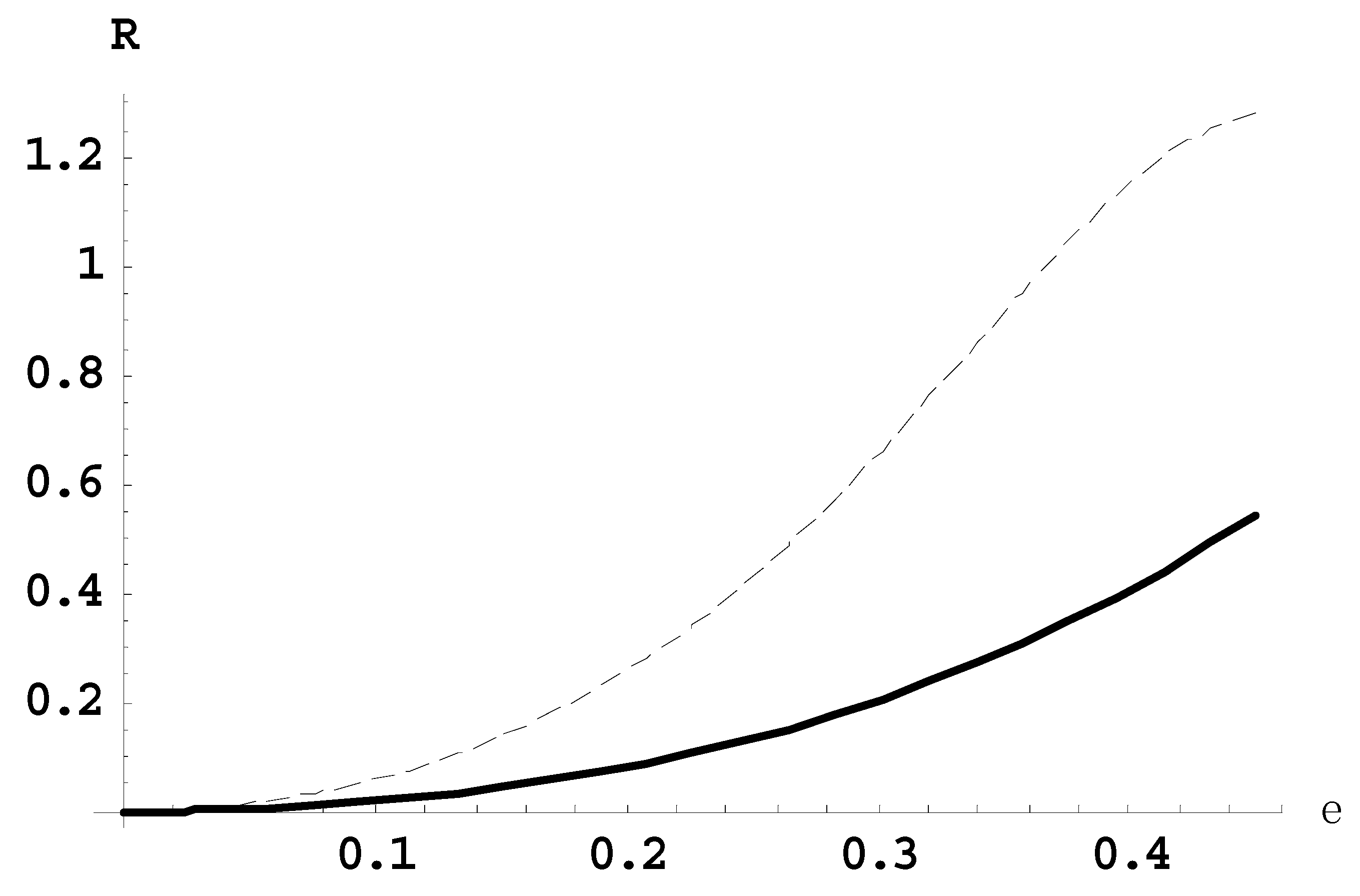
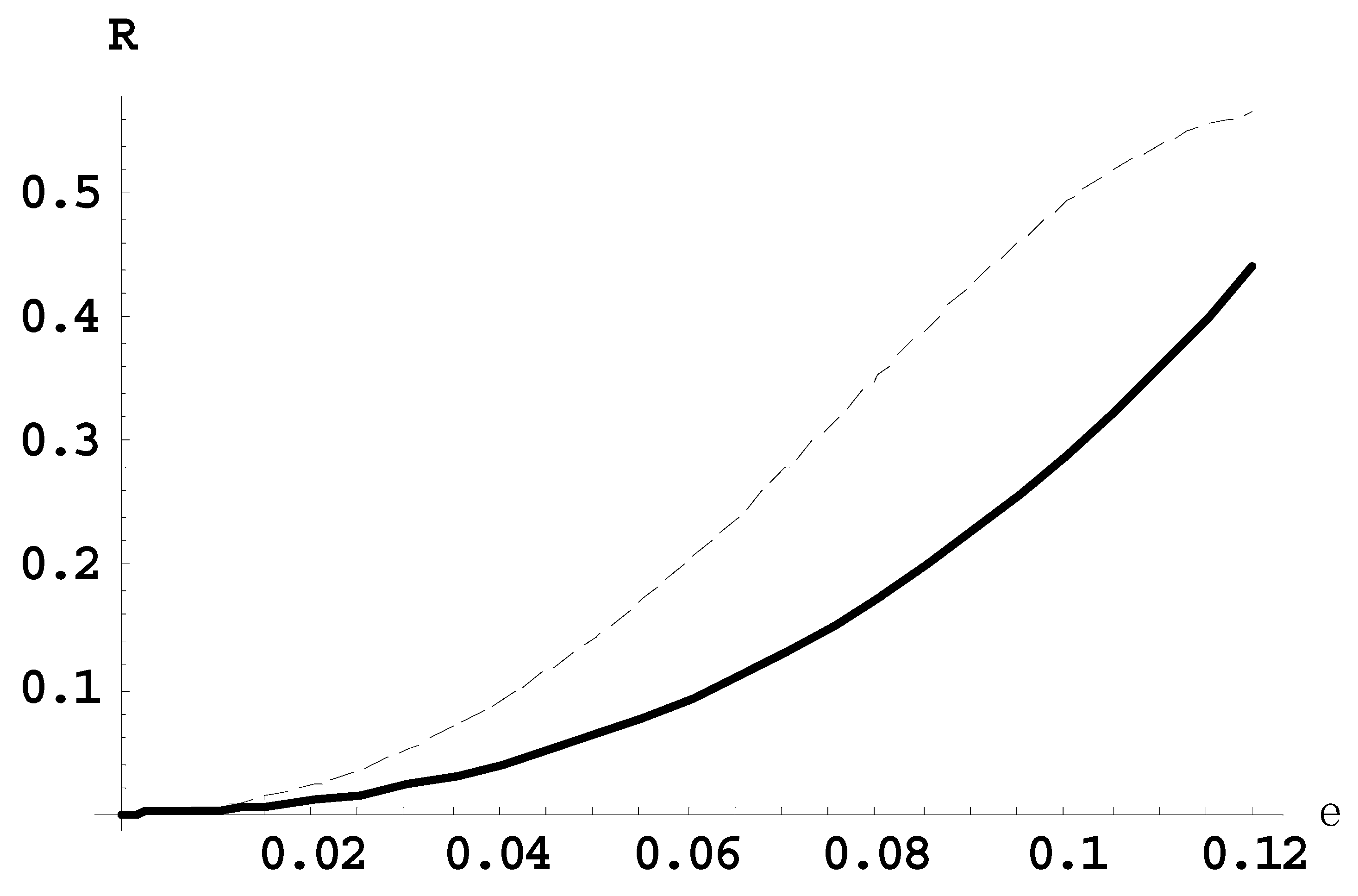
Figure 1 presents the dependence of the ratio R₂₁(ε) of the intensity of the second satellite to the intensity of the first satellite (solid line) and the ratio R₁₀(ε) of the intensity of the first satellite to the intensity of the main line (dashed line), for the Lyman-beta line for the observation perpendicular to the laser field.

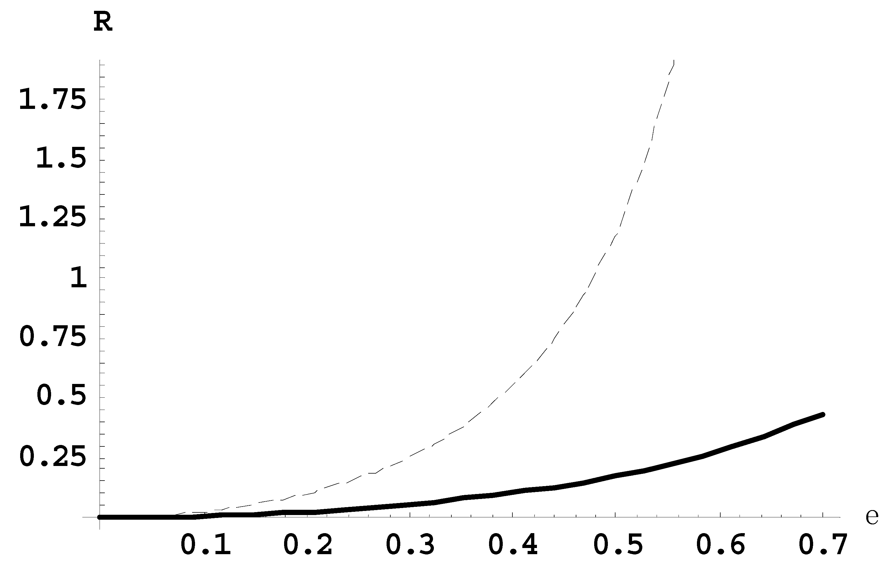
Figure 2 presents the dependence of the ratio R₂₁(ε) of the intensity of the second satellite to the intensity of the first satellite (solid line) and the ratio R₁₀(ε) of the intensity of the first satellite to the intensity of the main line (dashed line), for the Lyman-beta line for the observation parallel to the laser field.

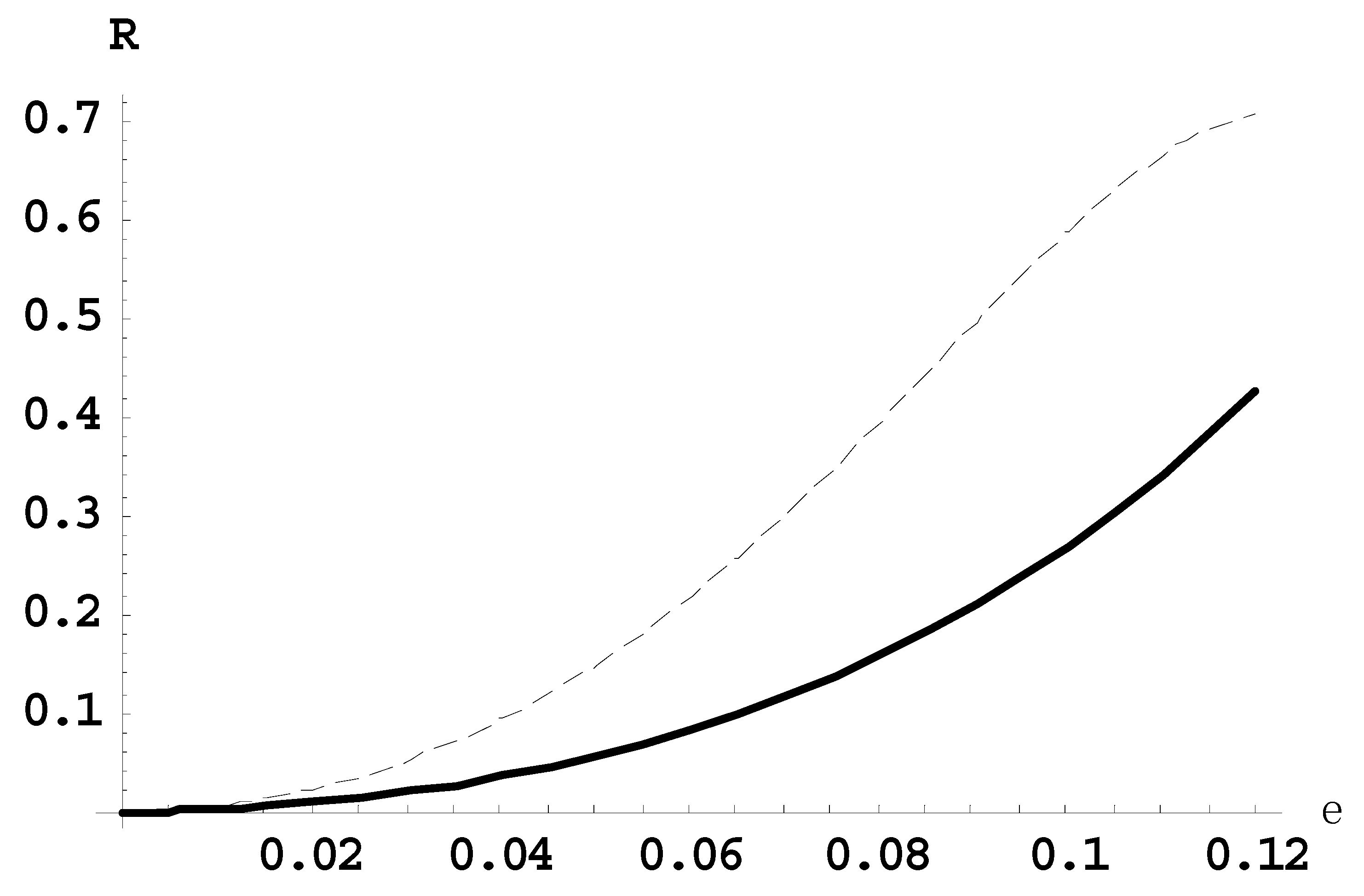
Figure 3 presents the dependence of the ratio R₂₁(ε) of the intensity of the second satellite to the intensity of the first satellite (solid line) and the ratio R₁₀(ε) of the intensity of the first satellite to the intensity of the main line (dashed line), for the Lyman-delta line for the observation perpendicular to the laser field.

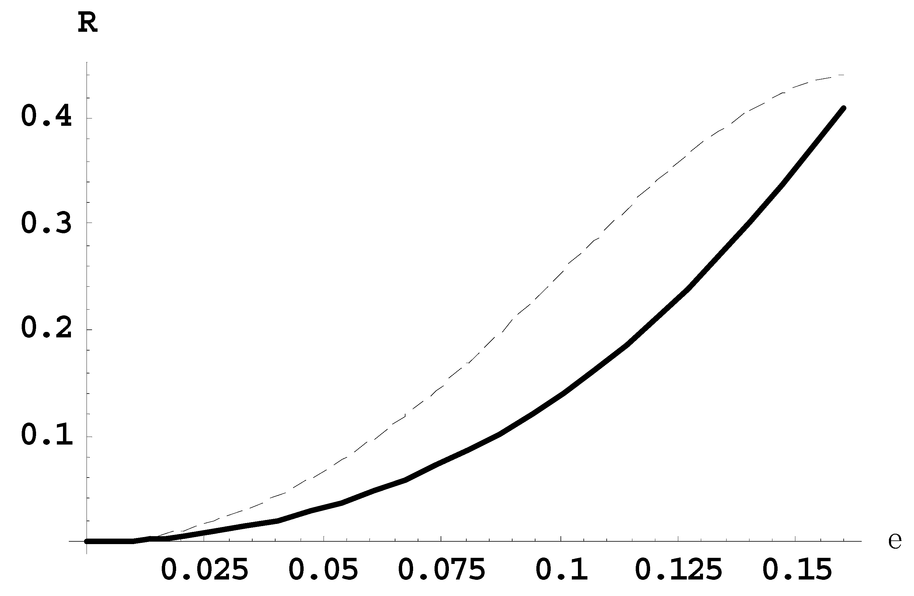
Figure 4 presents the dependence of the ratio R₂₁(ε) of the intensity of the second satellite to the intensity of the first satellite (solid line) and the ratio R₁₀(ε) of the intensity of the first satellite to the intensity of the main line (dashed line), for the Lyman-delta line for the observation parallel to the laser field.

Figure 5 presents the dependence of the ratio R₂₁(ε) of the intensity of the second satellite to the intensity of the first satellite (solid line) and the ratio R₁₀(ε) of the intensity of the first satellite to the intensity of the main line (dashed line), for the Balmer-beta line for the observation perpendicular to the laser field.

Figure 6 presents the dependence of the ratio R₂₁(ε) of the intensity of the second satellite to the intensity of the first satellite (solid line) and the ratio R₁₀(ε) of the intensity of the first satellite to the intensity of the main line (dashed line), for the Balmer-beta line for the observation parallel to the laser field.

Figure 7 presents the dependence of the ratio R₂₁(ε) of the intensity of the second satellite to the intensity of the first satellite (solid line) and the ratio R₁₀(ε) of the intensity of the first satellite to the intensity of the main line (dashed line), for the Balmer-delta line for the observation perpendicular to the laser field.

Figure 8 presents the dependence of the ratio R₂₁(ε) of the intensity of the second satellite to the intensity of the first satellite (solid line) and the ratio R₁₀(ε) of the intensity of the first satellite to the intensity of the main line (dashed line), for the Balmer-delta line for the observation parallel to the laser field.

All of the above figures demonstrate, in particular, the following. For relatively small laser fields, there is one-to-one correspondence between the scaled laser field ε and the corresponding ratios of satellite intensities.

Now we present the corresponding analytical results for the cases of the nonzero optical depth. At τ₀ > 0 (and especially at τ₀ > 1), the ratio R₁₀(τ₀) has to be calculated as follows.

In Equation (3) the profiles of each satellite and of the main line are represented by the delta-function. In reality, these profiles are influenced by various broadening mechanisms. Typically, for the experimental ratio of intensities of the satellites (to each other or to the intensity of the main line) one uses the corresponding experimental ratio of the peak intensities.

The profile P(Δω) of a spectral line affected by the optical thickness can be represented as follows

P(τ₀, Δω) = {1 − exp[−τ₀P₀(Δω)]}/τ₀,

(8)

where P₀(Δω) is the profile of the absorption coefficient normalized such that P₀(0) = 1. At τ₀ = 0, one has P(0, Δω) = P₀(Δω), so that P(0, 0) = 1. The peak intensity of the normalized profile is

P(τ₀, 0) = [1 − exp(−τ₀)]/τ₀.

(9)

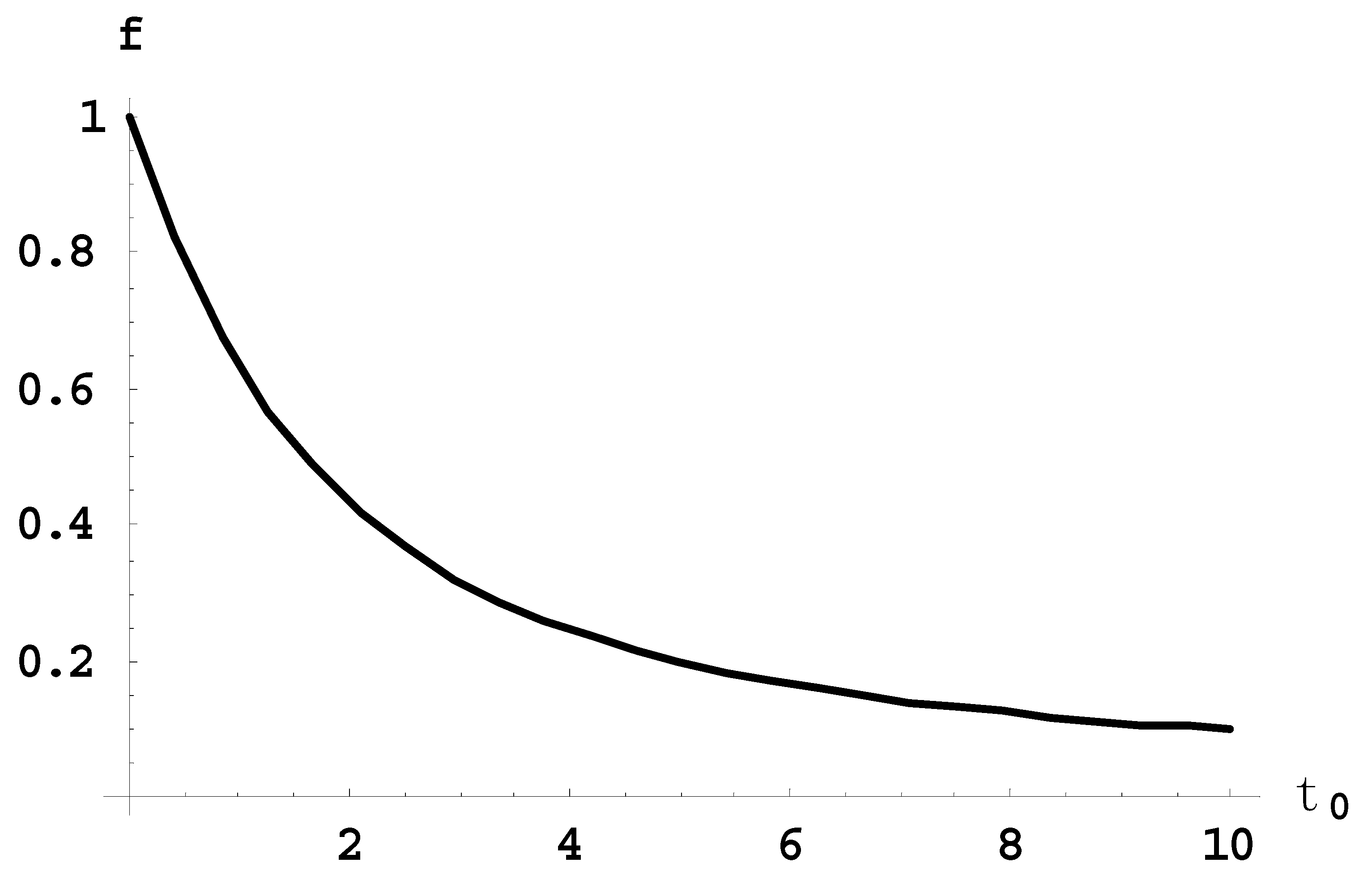
Thus, the factor reducing the peak intensity compared to the case of τ₀ = 0 is

f(τ₀) = [1 − exp(−τ₀)]/τ₀.

(10)

Figure 9 shows the dependence of the reducing factor f on the optical depth τ₀. It is seen the greater the optical depth, the more significant becomes the reduction of the peak intensity.

Since the satellites are optically thin and P(0, 0) = 1, the ratio of the peak intensity of the second satellite to the peak intensity of the first satellite is still given by Equation (6). But for the ratio of the peak intensity of the first satellite to the peak intensity of the main line we get

R₁₀(τ₀, ε) = I(1, ε)/[I(0, ε) f(τ₀)]

(11)

or

f(τ₀) = I(1, ε)/[I(0, ε) R₁₀(τ₀, ε)].

(12)

Thus, from the experimental ratio R₂₁ one can determine the scaled amplitude of the laser field ε (as well as the laser amplitude E₀ by using Equation (6)). Then after substituting the found value of ε and the experimental ratio R₁₀ in the right side of Equation (12), one can determine the optical depth τ₀ of the main line. For the frequently used spectral lines Lyman-beta, LyFigurean-delta, Balmer-beta, and Balmer-delta, the ratio I(1, ε)/I(0, ε) entering Equations (11) and (12) can be determined also from Figure 1, Figure 2, Figure 3, Figure 4, Figure 5, Figure 6, Figure 7 and Figure 8.

For resolving the satellites, the frequency of the laser field should significantly exceed the characteristic scales of the Stark and Doppler broadenings:

ω >> max[n²ħZ_p^1/3N_e^2/3/(Z_rm_e), ω₀(T/M)^1/2/c].

(13)

Here Z_p is the charge of perturbing ions, ω₀ is the unperturbed frequency of the spectral line, T is the ion temperature and M is the reduced mass of the pair “perturbing ion and radiating ion/atom”.

If ω is the frequency of the Nd laser (1.77 × 10¹⁵ s⁻¹), then for the Si XIV Ly-beta line (used, e.g., in experiments [17,18]), the condition (13) is satisfied for N_e << 3 × 10²³ cm⁻³ and T << 6 keV. Even in studies of relativistic laser-plasma interactions (such as, e.g., the studies [17,18]) both the N_e and T are by one or more orders of magnitude lower than the above thresholds, so that the condition (13) is met. In studies of nonrelativistic laser-plasma interactions (i.e., for lower laser intensities), both the N_e and T are lower than in the relativistic situation, so that the condition (13) is satisfied with even broader margin. Therefore, the employment of the satellites of hydrogenic spectral lines for the diagnostic presented in this paper should be feasible in experiments like [13,14].

3. Conclusions

We presented the method allowing to measure both the laser field and the opacity from experimental spectrum of a hydrogenic line exhibiting satellites. The method is appropriate for a linearly-polarized laser field at the surface of the critical density or in underdense plasma regions. We derived the necessary theoretical results analytically and showed how to use them for this purpose. This spectroscopic diagnostic should be useful for a better understanding of laser-plasma interactions, including relativistic laser-plasma interactions. The spectral lines chosen as the examples, are most sensitive to the described effects and therefore most appropriate for implementing this new diagnostic method.

To the best of our knowledge, this is the only one method allowing to measure simultaneously both the laser field and the opacity from the spectral line shapes. This makes it advantageous compared to other methods.

We note that recent spectroscopic studies of relativistic laser-plasma interactions [17,18] showed that a spatial inhomogeneity of the laser-produced plasmas does not play a significant role, because the primary contribution to the intensity of the experimental spectral lines originates from a relatively small (and therefore, quasi-homogeneous) layer around the surface of the relativistic critical density. Otherwise, the L-dips, caused by the Langmuir waves (the waves developing only at the surface of the relativistic critical density via the parametric decay instability)—the L-dips clearly identified in the experimental x-ray line profiles—would have been smeared out by the contribution from other layers where the Langmuir waves could not develop.

References

- Maine, P.; Strickland, D.; Bado, P.; Pessot, M.; Mourou, G. Generation of ultrahigh peak power pulses by chirped pulse amplification. IEEE J. Quantum Electron. 1988, 24, 398–403. [Google Scholar] [CrossRef]
- Akhiezer, A.I.; Polovin, R.V. Theory of Wave Motion of an Electron Plasma. Sov. Phys. JETP 1956, 3, 696–705. [Google Scholar]
- Lünow, W. On the relativistic non-linear interaction of cold plasma with electro-magnetic waves. Plasma Phys. 1968, 10, 879–890. [Google Scholar] [CrossRef]
- Guerin, S.; Mora, P.; Adam, J.C.; Heron, A.; Laval, G. Propagation of ultraintense laser pulses through overdense plasma layers. Phys. Plasmas 1996, 3, 2693–2699. [Google Scholar] [CrossRef]
- Oks, E. Diagnostics of Laboratory and Astrophysical Plasmas Using Spectral Lines of One-, Two-, and Three-Electron Systems; World Scientific: Singapore, 2017. [Google Scholar]
- Kunze, H.-J. Introduction to Plasma Spectroscopy; Springer: Berlin, Germany, 2009. [Google Scholar]
- Oks, E. Stark Broadening of Hydrogen and Hydrogenlike Spectral Lines in Plasmas: The Physical Insight; Alpha Science International: Oxford, UK, 2006. [Google Scholar]
- Fujimoto, T. Plasma Spectroscopy; Clarendon Press: Oxford, UK, 2004. [Google Scholar]
- Salzman, D. Atomic Physics in Hot Plasmas; Oxford University Press: Oxford, UK, 1998. [Google Scholar]
- Griem, H.R. Principles of Plasma Spectroscopy; Cambridge University Press: Cambridge, UK, 1997. [Google Scholar]
- Oks, E. Plasma Spectroscopy: The Influence of Microwave and Laser Fields; Springer Series on Atoms and Plasmas: New York, NY, USA, 1995; Volume 9. [Google Scholar]
- Oks, E. Review of Recent Advances in the Analytical Theory of Stark Broadening of Hydrogenic Spectral Lines in Plasmas: Applications to Laboratory Discharges and Astrophysical Objects. Atoms 2018, 6, 50. [Google Scholar] [CrossRef] [Green Version]
- Elton, R.C.; Griem, H.R.; Welch, B.L.; Osterheld, A.L.; Manchini, R.C.; Knauer, J.; Pien, G.; Watt, R.G.; Cobble, J.A.; Jaanimagi, P.A.; et al. Satellite spectral lines in high density laser-produced plasmas. J. Quant. Spectrosc. Radiat. Transf. 1997, 58, 559–570. [Google Scholar] [CrossRef]
- Sauvan, P.; Dalimier, E.; Oks, E.; Renner, O.; Weber, S.; Riconda, C. Spectroscopic diagnostics of plasma interaction with an external oscillatory field. J. Phys. B At. Mol. Opt. Phys. 2009, 42, 195001. [Google Scholar] [CrossRef]
- Blochinzew, D.I. Zur Theorie des Starkeffektes im Zeitveränderlichen Feld. Phys. Z. Sov. Union 1933, 4, 501–515. [Google Scholar]
- Oks, E. Spectroscopy of plasmas containing quasimonochromatic electric fields. Sov. Phys. Doklady 1984, 29, 224–226. [Google Scholar]
- Oks, E.; Dalimier, E.; Faenov, A.Y.; Angelo, P.; Pikuz, S.A.; Pikuz, T.A.; Skobelev, I.Y.; Ryazanzev, S.N.; Durey, P.; Doehl, L.; et al. In-Depth Study of Intra-Stark Spectroscopy in the X-Ray Range in Relativistic Laser-Plasma Interactions. J. Phys. B At. Mol. Opt. Phys. 2017, 50, 245006. [Google Scholar] [CrossRef] [Green Version]
- Oks, E.; Dalimier, E.; Faenov, A.Y.; Angelo, P.; Pikuz, S.A.; Tubman, E.; Butler, N.M.H.; Dance, R.J.; Pikuz, T.A.; Skobelev, I.Y.; et al. Using X-ray spectroscopy of relativistic laser plasma interaction to reveal parametric decay instabilities: A modeling tool for astrophysics. Opt. Express 2017, 25, 1958. [Google Scholar] [CrossRef] [PubMed] [Green Version]
Figure 1.
Ratio R21 of the intensity of the second satellite to the intensity of the first satellite (solid line) and the ratio R10 of the intensity of the first satellite to the intensity of the main line (dashed line) versus the scaled dimensionless laser field ε, for the Lyman-beta line for the observation perpendicular to the laser field.
Figure 2.
The same as in Figure 1, but for the observation parallel to the laser field: solid line is R21; dashed line is R10.
Figure 3.
Ratio R21 of the intensity of the second satellite to the intensity of the first satellite (solid line) and the ratio R10 of the intensity of the first satellite to the intensity of the main line (dashed line), versus the scaled dimensionless laser field ε, for the Lyman-delta line for the observation perpendicular to the laser field.
Figure 4.
The same as in Figure 3, but for the observation parallel to the laser field: solid line is R21; dashed line is R10.
Figure 5.
Ratio R21 of the intensity of the second satellite to the intensity of the first satellite (solid line) and the ratio R10 of the intensity of the first satellite to the intensity of the main line (dashed line), versus the scaled dimensionless laser field ε, for the Balmer-beta line for the observation perpendicular to the laser field.
Figure 6.
The same as in Figure 5, but for the observation parallel to the laser field: solid line is R21; dashed line is R10.
Figure 7.
Ratio R21 of the intensity of the second satellite to the intensity of the first satellite (solid line) and the ratio R10 of the intensity of the first satellite to the intensity of the main line (dashed line), versus the scaled dimensionless laser field ε, for the Balmer-delta line for the observation perpendicular to the laser field.
Figure 8.
The same as in Figure 7, but for the observation parallel to the laser field: solid line is R21; dashed line is R10.
Figure 9.
Dependence of the factor f, reducing the peak intensity of spectral line profiles, on the optical depth τ0.
Publisher’s Note: MDPI stays neutral with regard to jurisdictional claims in published maps and institutional affiliations. |
© 2021 by the author. Licensee MDPI, Basel, Switzerland. This article is an open access article distributed under the terms and conditions of the Creative Commons Attribution (CC BY) license (http://creativecommons.org/licenses/by/4.0/).
Share and Cite
MDPI and ACS Style
Oks, E. Method for Measuring the Laser Field and the Opacity of Spectral Lines in Plasmas. Plasma 2021, 4, 65-74. https://0-doi-org.brum.beds.ac.uk/10.3390/plasma4010003
AMA Style
Oks E. Method for Measuring the Laser Field and the Opacity of Spectral Lines in Plasmas. Plasma. 2021; 4(1):65-74. https://0-doi-org.brum.beds.ac.uk/10.3390/plasma4010003
Chicago/Turabian StyleOks, Eugene. 2021. "Method for Measuring the Laser Field and the Opacity of Spectral Lines in Plasmas" Plasma 4, no. 1: 65-74. https://0-doi-org.brum.beds.ac.uk/10.3390/plasma4010003