Article

The Effect of Surface Fire in Savannah Systems in the Kruger National Park (KNP), South Africa, on the Backscatter of C-Band Sentinel-1 Images

1
Ecosystem Earth Observation, Natural Resources and the Environment, Council for Science and Industrial Research, PO BOX 395, Pretoria 0001, South Africa
2
Department of Geography, Geomatics and Meteorology, University of Pretoria, Lynnwood Rd, Hatfield, Pretoria 0002, South Africa
3
Department of Geography, Environment & Spatial Sciences and Center for Global Change and Earth Observations, Michigan State University, East Lansing, MI 48824, USA
4
Department of Chemistry, Princeton University, Princeton, NJ 08544, USA
*
Author to whom correspondence should be addressed.
Submission received: 11 April 2019 / Revised: 3 June 2019 / Accepted: 14 June 2019 / Published: 27 June 2019
(This article belongs to the Special Issue Remote Sensing of Fire and Its Impact on Land and Atmosphere)

Abstract

:
Savannahs are mixed woody-grass communities where low-intensity surface fires are common, affecting mostly the grass layer and rarely damaging trees. We investigated the effect of surface fires in a savannah system in the Kruger National Park, South Africa, on the backscatter of synthetic aperture radar (SAR) C-band Sentinel-1A images. Pre-fire and post-fire dual polarized (VH, VV) C-band backscatter values were examined for 30 burn events. For all events, a systematic backscatter decrease from pre-fire to post-fire conditions was observed, with mean backscatter decreases of 1.61 dB and 0.99 dB for VH and VV, respectively. A total of 90% and 75% of the burn events showed a decrease in VH and VV backscatter greater than 0.43 dB, the overall absolute radiometric of Sentinel-1A products. The VH data were, overall, 1.7 times more sensitive to surface fire effects than the VV data. C-band data are likely sensitive to a reduction in grass biomass typical of surface fires, as well as in grass/soil moisture levels. Early season fires had higher backscatter decreases due to greater early season moisture conditions. For region with more than 30% woody cover, the effect of fire on the C-band backscatter was reduced. Denser woody communities tend to produce lower grass fuel load and less intense surface fires, and limit the penetration of C-band microwaves to the ground where most savannah fires and associated effects occur. This research provides evidence that C-band space-borne SAR is sensitive to the effects of surface-level fires in southern African savannahs. The unique availability of frequent and spatially detailed C-band data from the Sentinel-1 SAR constellation provide new opportunities for burned area mapping and systematic monitoring in savannahs systems, for instance, for fine-scale fire propagation studies.

1. Introduction

Globally, fires occur more in savannahs than in any other biome [1,2]. They emit large quantities of aerosols and greenhouse gases [3] and are an important vegetation disturbance [4]. Fire is an integral part of African savannah ecosystems [5,6] and include natural fires (lightning) and a majority of anthropogenic fires, ignited for instance for land clearing, enhancing livestock productivity, bush control, and arson or accidents [7,8,9]. The fire intensity and frequency may alter the long-term woody/grass cover ratio, woody height profile, and short- to long-term surface albedo [10,11,12,13], with potentially cascading effects on water and nutrient cycling, biodiversity, resource availability (e.g., grazing or fuelwood), energy balance, and climate variability [14,15,16,17]. Spatially and temporally explicit maps of burned area are needed to estimate aerosols and gaseous emissions for modelling climate variability, carbon budgets, pollutant transport, and air quality [3,18,19,20], and to improve our understanding of fire processes and impacts on ecosystem services [21,22]. Improved knowledge on fire occurrence may support the development of policies, management strategies, and operations to enhance its effective use, control, and protection against fire [23,24,25].
The extent of burned areas can be mapped using remote sensing by detecting fire-induced changes including the deposition of char and ash, removal of standing vegetation and debris, and changes to the vegetation structure [26]. Burned area products over large areas have been produced from a range of optical wavelength satellite remote sensing data [27], especially from coarse spatial resolution and high temporal frequency sensors, such as NOAA AVHRR [28], MODIS [29], SPOT Vegetation [30], or ENVISAT MERIS [1], and more recently using medium spatial but low temporal resolution Landsat imagery [31,32]. It is well established, however, that optical wavelength burned area detection algorithms are limited by cloud obscuration and optically thick smoke [2]. Synthetic aperture radar (SAR) can sense through clouds and smoke and SAR data have been used to assess the extent of fires in different forest systems including tropical forests [33,34,35], boreal forests [36,37,38], temperate forests [39], and Mediterranean landscapes [40,41,42]. SAR systems operating within the microwave domain (from X- to P-band) are sensitive to tree structure, thus, they are useful for mapping burned areas in dense forests where canopy fires severely affect tree canopy structure. In addition, SAR may also provide a useful tool to document post-fire recovery processes such as tree regrowth [43,44,45]. Although L-band is more sensitive to tree structural changes [46], C-band data (e.g., ENVISAT ASAR, RADARSAT) were often used for the detection of burned areas in forest biomes due to the lack of frequent L-band SAR time series to date.
Savannah vegetation consists of mixed woody-grass communities, with a semi-continuous grass layer and a woody cover varying from 10% to 60% [47]. African savannah fires are predominantly surface fires (as opposed to canopy fires) that burn mostly grasses, shrubs, and woody debris accumulated over the growing season and in preceding fire-free growing seasons [48]. Surface fires remove the grass layer while woody canopies are minimally affected, as fires only rarely reach the tree canopy [49,50,51]. African savannah fires are generally of lower intensity but occur at higher frequency than in tropical, boreal, or temperate forests, due to the higher rates of regrowth of the main grass fuel source [52].
Menges et al. [53] investigated the effect of fire on microwave backscatter in a predominantly savannah landscape in Australia using a single airborne multi-frequency (C-, L-, P-band) dataset. They concluded that of the three SAR frequencies considered, only the C-band was affected significantly by fire effects. Comparing unburnt and burnt patches using C-band VV imagery (VH or HV was not available), they showed that the SAR backscatter decreased by 0.62 dB and 1.21 dB for woodland and grassland, respectively. The burning of the senesced grass layer may decrease the C-band backscatter as this frequency is sensitive to changes in small-size scatterers of a similar size as grass foliage [46]. Since fire-driven tree and shrub structural changes are limited, L- and P-bands are less effective for detecting fire-related changes in savannas. Cross-polarized VH or HV C-band SAR backscatter may be more sensitive than the VV polarized data used by [53] due to its higher sensitivity to changes in grass volume scattering [54].
The availability of frequent high-spatial-resolution C-band (5.6 cm) Sentinel-1A (launched 2014) and Sentinel-1B (launched 2016) SAR satellite data [55] have opened up new SAR burned area monitoring opportunities, especially in savannahs. The interferometric wide swath Sentinel-1 mode data are acquired in dual polarimetric configuration with VV and VH polarizations and a spatial resolution of approximately 5 × 20 m. The two Sentinel-1 satellites have a six-day equatorial revisit, which is comparable to the revisit provided by combination of Sentinel-2A, Sentinel-2B, and Landsat-8 optical wavelength data assuming 50% cloud cover at the time of overpass [56]. Prior to Sentinel-1, frequent (every 2 weeks) global coverage SAR data with a high level of spatial detail (<1 ha) and of free access were not available. As a result, the potential of satellite C-band SAR data for the systematic monitoring of the occurrence of surface fires needs to be more widely assessed. Indeed, only one recent investigation used Sentinel-1 (together with Sentinel-2) time-series data to monitor burnt areas in tropical evergreen forests, including open forests with tall grasses [35].
In this study, the effect of surface fire in savannah systems in the Kruger National Park (KNP), South Africa, on C-band Sentinel-1 images were examined. Thirty burned areas across the park that occurred at different times in 2015 were considered to provide a comprehensive study set. The burned areas were identified using a 500 m MODIS-based burned area dataset, and then more accurately delineated using 30 m Landsat 8 data to enable appropriately detailed comparison with the Sentinel-1 data. Changes in the Sentinel-1 VV and VH C-band backscatter were examined to investigate the effect of fire disturbance on the backscatter of Sentinel-1 images. Temporal backscatter dynamics were analyzed in the context of rainfall and phenology that were impacted by the exceptional 2015 KNP drought. The seasonality of pre-fire to post-fire differences, and also the effect of woody cover, were examined as C-band SAR data are known to be sensitive to soil moisture and vegetation moisture and to woody structure [57,58].

2. Materials and Methods
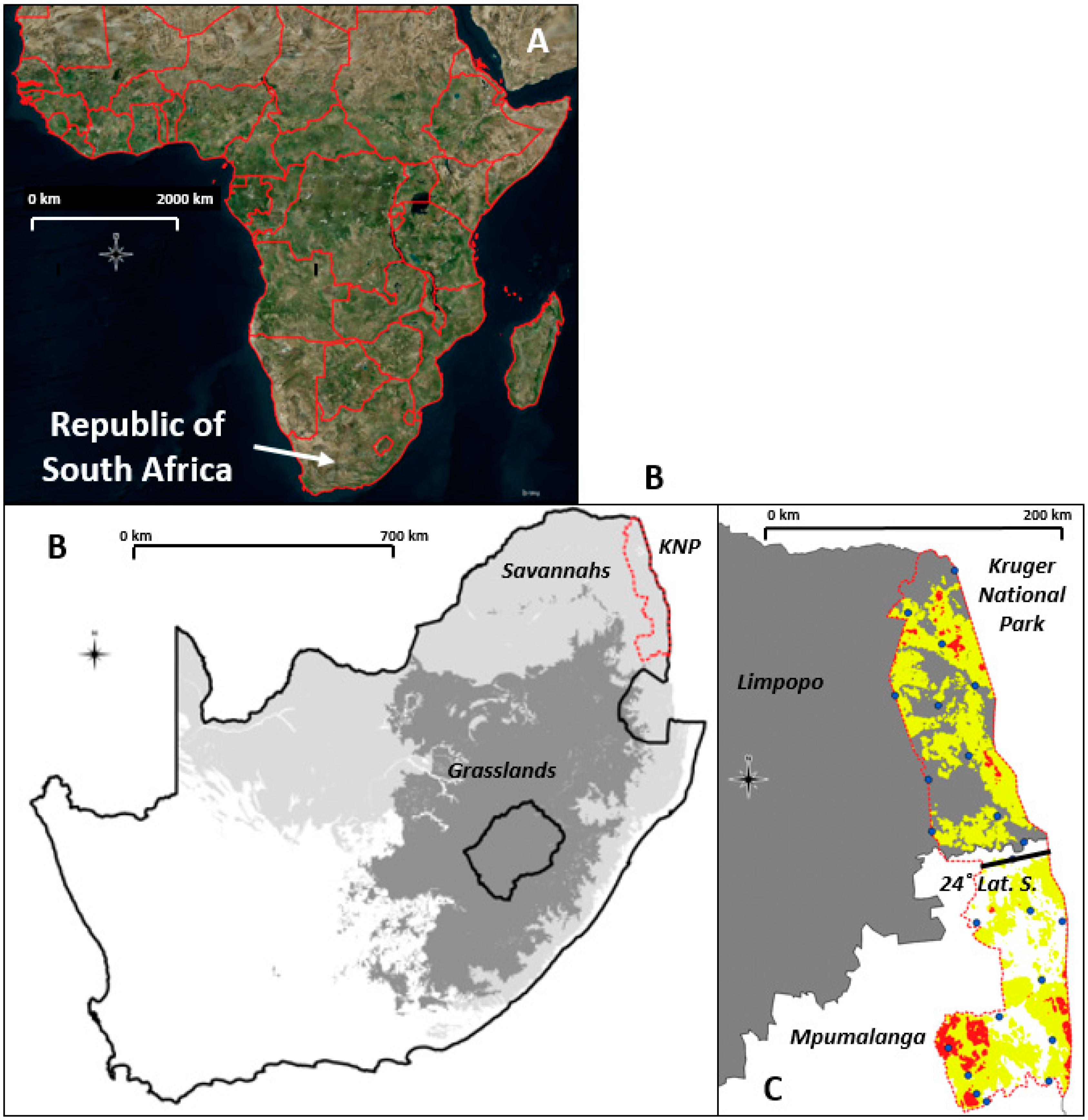
2.1. Study Area

The KNP is the largest public protected area in South Africa (1.95 million ha) and is located in the north-eastern corner of the country bordering Mozambique and Zimbabwe (Figure 1). It is the largest conservation area in South Africa and is considered to be one of the most pristine semi-arid savannahs in the region. Human presence and activities in the park are mostly related to conservation tourism. Environmental conditions in the park (rainfall, geology, woody cover/bushiness) are diverse, and fire is common, making it an ideal site for the purpose of this study. The KNP climate is subtropical with two contrasting seasons, a dry season from April to September (mean daily minimum and maximum temperatures of 10 °C and 27 °C) and a wet and hot season from October to March (mean daily minimum and maximum temperatures of 23 °C to 34 °C). Mean annual precipitation (MAP) has an increasing north–south gradient from 350 to 700 mm [59]. Rainfall events are spatially and temporally heterogeneous and are generally due to convective thunderstorms. Elevation ranges from about 260 m above sea level in the east to 840 m in the south-western areas of the park. The dominant geology includes nutrient-rich basalts in the eastern plains and nutrient-poor granites and gneisses in the west. The hydrological network is structured around six perennial rivers (Limpopo, Luvuvhu Letaba, Olifant, Sabie, Crocodile) draining eastward into the Indian Ocean with a dense network of seasonally flowing tributaries. Woodlands and grasslands dominate the park vegetation with a canopy cover ranging from 10% to 60%, and more than 80% in thin riparian zones [60]. Grass-dominated versus woody-dominated regional vegetation patterns are controlled by rainfall and geological gradients with finer scale variations, driven by geomorphology (catenas) and disturbance history, e.g., large herbivores, mainly elephants [61,62], and fire [63,64]. In granitic areas, woody communities are dominated by moderately dense broad leaf deciduous trees in deep sandy uplands and dense thicket to open savanna in lowlands [65]. The vegetation in the basaltic landscapes forms large tracks of palatable grassland with low density of shrubs and scattered larger fine leaf trees.
In the park, various fire management policies have been implemented since 1941 [66], from no management intervention at all (natural fires only) to a command-and-control fire strategy aimed at prescribed burning of fixed management areas every three years. Since 2002, an outcomes-based integrated fire management policy is in place. The strategy allows managers, depending on range conditions, to burn patch mosaics, which, together with natural fires (lightning), aim to maintain biodiversity and vegetation heterogeneity. Between 2000 and 2010, 60% of the park was burned every three to five years and 5% every two years (Figure 1).
The photographs in Figure 2 show examples of typical pre-fire and post-fire surface conditions in South African savannahs; char and ash are deposited through the burning and removal of dry grasses and debris, and the tree or shrubs above the flame height are minimally affected. Wind and rain may blow away the char and ash to reveal the understory and soil.

2.2. Remote Sensing Data

Sentinel-1A was launched in April 2014, and, following the commissioning phase, started to acquire data over the KNP in March 2015. A total of 19 interferometric wide (IW) swath Sentinel-1A C-band images acquired in the afternoon over the KNP (16.30 overpass local time) from 20 March 2015 to 14 January 2016 were considered. The images were available in dual polarimetric mode (VV, VH) and at 10 × 10 m pixel spacing (Level-1 ground range detected). The images were sensed typically every 12 days, although some consecutive images had 24- or 36-day intervals. The look angle (i.e., the angle between the slant range and SAR instrument nadir) ranged from 37.8° (near range) to 43.7° (far range) and the mean angle per image date changed by less than 1° over the time series. These angles are relative to the KNP boundaries, which extend, at most, 80 km from the west to the east. This configuration provides a good compromise between small incidence angles, which enable more penetration of woody canopies and large incidence angles, which are more sensitive to herbaceous and woody vegetation structure [67]. A Sentinel-1A system calibration assessment was performed by the German Space Agency using corner reflectors and transponders, and the overall absolute radiometric accuracy of Sentinel-1A products for the mission time was assessed to be 0.43 dB (1σ) for all modes (Stripmap, IW and Extra Wideswath), and across look angles [68].
The MODIS 8-day 500-m normalized difference vegetation index (NDVI) product [69] was used to examine vegetation phenological changes with temporal changes in the Sentinel-1A backscatter values. The long-term mean and standard deviation (STD) NDVI values for 2000 to 2015, and for the 2015 data corresponding to the SAR data used in this study, were extracted, taking care to remove the low quality and cloud flagged NDVI values. A 2015 500-m MODIS-based burned area dataset, produced by the CSIR (South Africa) and disseminated by the active fire information system (AFIS) (https://southernafrica.afis.co.za/) was used to identify all the burn events, which occurred during the year 2015. It merges the MODIS MCD45A1 [2] and the MCD64A1 [70] 500 m burned area products over South Africa, and has been shown to improve the detection of burned areas, particularly of small burns [71]. The MODIS burned area products report the 500 m location of burning and the approximate date of burning with a median temporal reporting precision of 1 day [72]. The MODIS 1 km active fire detection product MCD14ML was also used that provides the center of each 1 km MODIS Terra or Aqua day or night observation flagged by the MODIS active fire detection algorithm as a fire, and includes a fire detection confidence score (0 to 100) [73]. Landsat 8 operational land imager (OLI) 30 m images were used to more accurately delineate the 500 m MODIS burned areas. Collection 1 Landsat 8 OLI Tier 1 images, which are geometrically corrected to ≤12 m root mean square error geodetic accuracy, and include a per-pixel cloud and shadow mask [74,75], were used. Each OLI image covers approximately 180 × 185 km and were available typically every 16 days over the KNP.

2.3. Ancillary Data

To understand potential moisture effects, daily rainfall data from 24 weather stations scattered across the KNP [76] were used (Figure 1). For some of the analyses, the rainfall was partitioned into 12 stations in the northern and southern sections (divided along 24°S, see Figure 1), and for other analyses, the rainfall data derived from the weather station closest to the burn event were used. Also, depending on the analysis, the daily rainfall data were aggregated at different time scales: The 8-day MODIS NDVI product reporting period, or the 7, 5, 3, or 1 days prior to each SAR image acquisition.
A KNP 1-ha scale woody cover (0%–100%) map was used to analyze the potential effect of woody vegetation cover on SAR burned area detection. The map was generated by random forest classification of L-band dual polarized (HH, HV) fine-resolution (9.4 × 3.2 m) ALOS PALSAR scenes acquired in 2010 and using 80,000 ha of LiDAR tracks acquired in 2012 for training and validation [77]. The woody cover map was produced at a 25 m pixel size and with an RMSE accuracy of 10.3% and a relative RMSE accuracy of 29.3%. The map was aggregated at a 100 m pixel size (1 ha) to further reduce noise and better match landscape variation of woody patches along catenae.

2.4. Methods

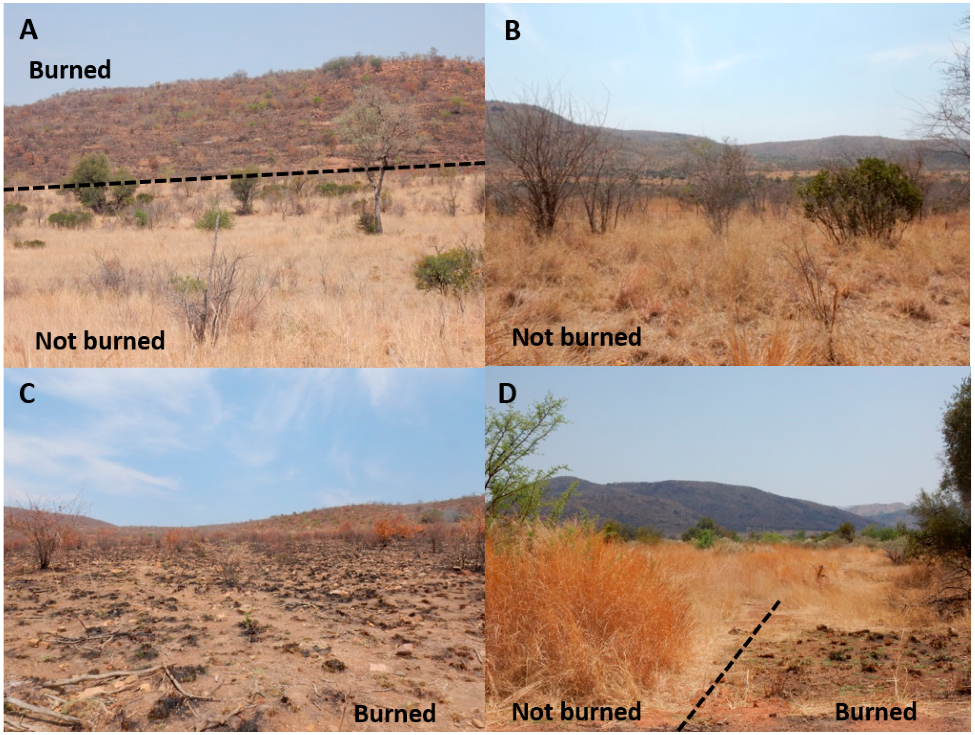
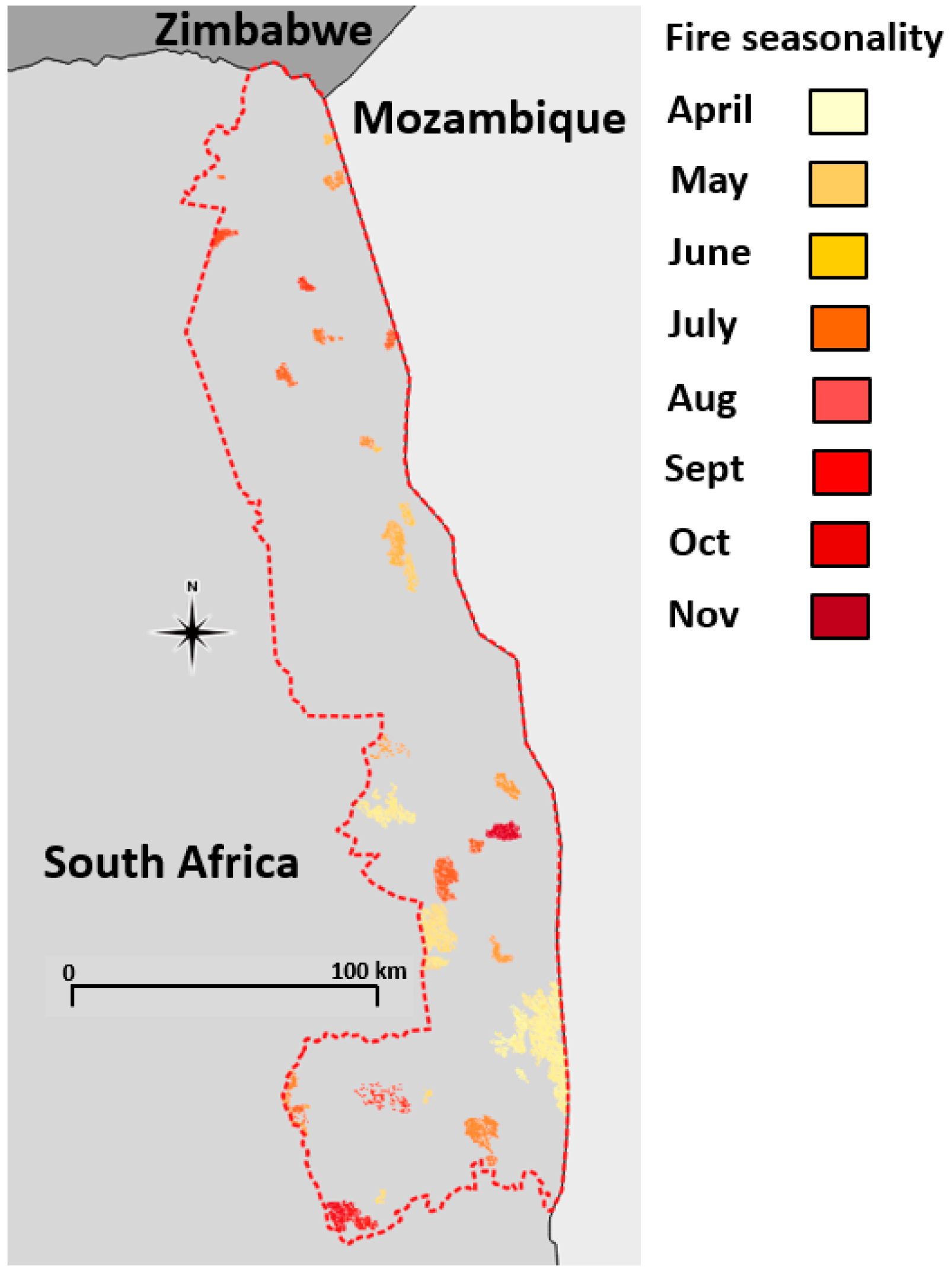
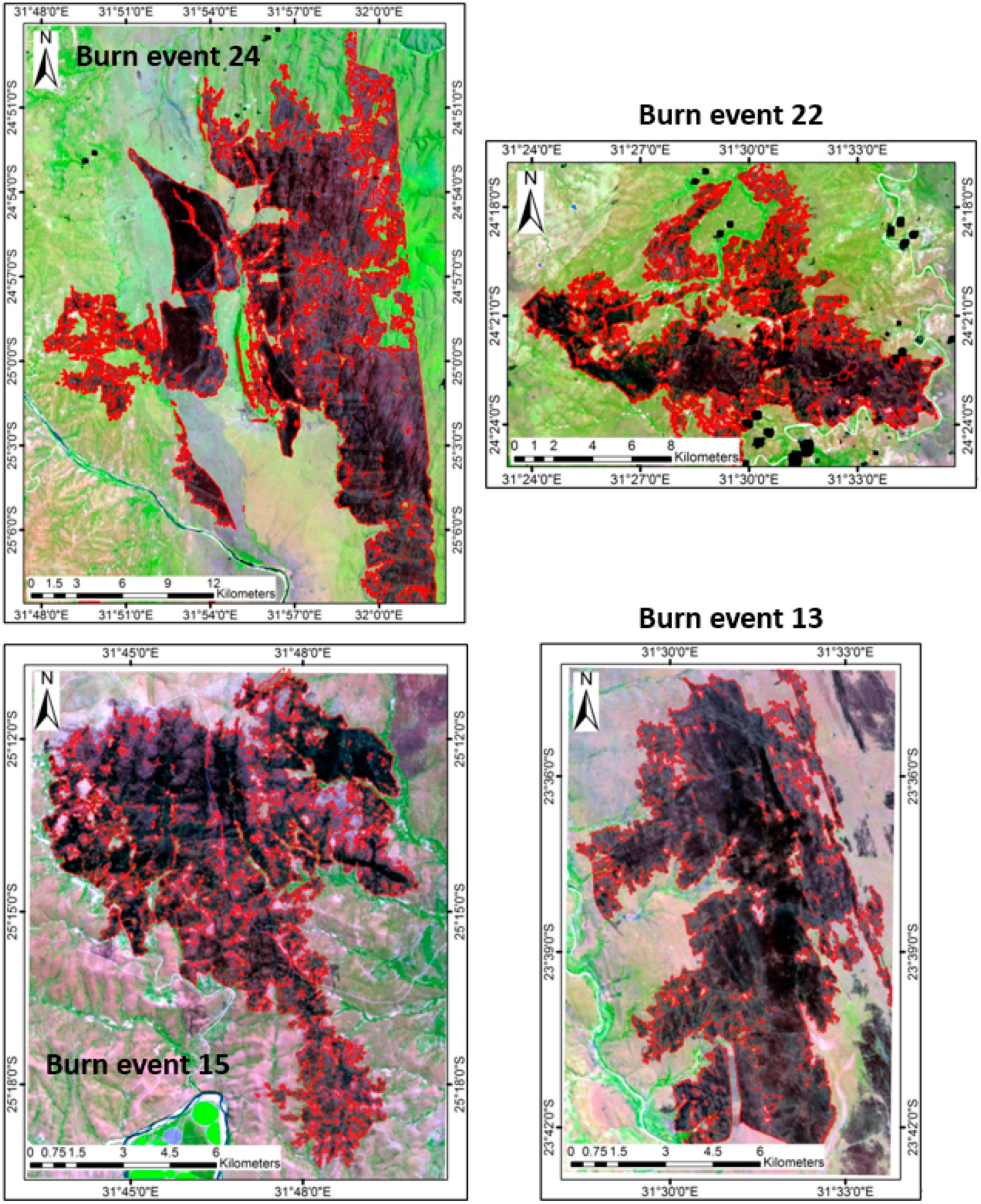
2.4.1. Burned Area Selection and Refinement

Burned areas were inventoried by examination of the MODIS burned area product data. Burned polygons were assigned to a single fire event, following the same approach as [78], if they were spatially contiguous or in close proximity (no more three 500-m pixels to each other) and occurred within one day of each other. In addition, only burned areas containing at least one high-confidence (confidence >50) MODIS 1 km active fire detection flag were retained. A total of 31 burn events were identified from February to December 2015 (Figure 3). The first February burn event was excluded as it occurred before the first KNP Sentinel-1A image was acquired. The 30 remaining burn events were categorized as belonging to the early fire season (i.e., before June, nine burn events), during the main fire season (June to August, 19 burn events), or the late fire season (after August, two burn events). This seasonality classification was derived from fire temporal frequency data derived for southern Africa [5].
Landsat 8 OLI 30 m images were used to more accurately delineate the 500 m MODIS burned areas. The delineation was undertaken by segmenting the images into burned and unburned segments using a simple segmentation approach, and then interactively cleaning and refining the burned areas visually. We assumed that the Landsat 8 pixels mapped as burned included only limited unburned material (and were not generally mixed pixels). The Otsu segmentation approach was applied to the Landsat 8 near infrared band. The method selects a local threshold value in a bimodal pixel distribution by minimizing the intra-class variance, thereby enabling a two-class segmentation [79]. The threshold was identified for each burn event separately, and to reduce pixel confusion, digitized regions of interest around each fire were used to spatially constrain the pixels on which the method operated. The binary segmentations were converted to a vector layer, and then interactively ‘cleaned’ of erroneous burned patches (e.g., water surfaces and topographic shadow), with the help of the Landsat 8 color composites. Figure 4 illustrates some example Landsat 8 OLI images and the resulting refined burned area vectors.
For the 30 burn events, the mean area (as measured by Landsat data) was 3500 ha (standard deviation STD 5300 ha), with a minimum and a maximum area of 255 ha and 29,500 ha, respectively. The mean fire duration (as measured by MODIS data) was 10.5 days (STD 4.8 days), with a minimum and maximum duration of 4 and 20 days, respectively.

2.4.2. Sentinel-1 Data Processing

The Sentinel-1A images were processed using the ESA sentinel application platform (SNAP) software (v4.1.1, http://step.esa.int). The following processing steps were undertaken in SNAP: Radiometric calibration to sigma nought (defined as the average value of the scattering cross-section per unit area [80]), topographic backscatter normalization, terrain correction using the “Range Doppler Terrain Correction” algorithm, and the shuttle radar topography mission (SRTM) 1-arc second (30 m) digital elevation model (DEM). The 10 × 10 m SAR images were multi-looked and aggregated to 100 m pixel size (1 ha) and converted from intensity to decibels (dB) [81]. The 100 m pixel size reduced the speckle noise to an average equivalent number of looks (ENL) of 53. The latter ENL value was calculated by dividing the mean square backscatter intensity by the variance (e.g., ENL = mean2/variance) over homogeneous grassland and wooded areas selected and averaged from two wet season and two dry season multi-looked images.

2.4.3. Pre-Fire and Post-Fire SAR Backscatter Analysis

The ability of the Sentinel-1A data to discriminate between burned and unburned areas was assessed by measuring backscatter (dB) differences between the Sentinel 1A pre-fire and post-fire images acquired as close as possible before the start and the end of each burn event, respectively. Only Sentinel-1 pixels completely within the boundary of the Landsat burn vector boundaries were analyzed to ensure that only “pure” fire affected pixels were considered. The mean time lag between the pre-fire image and the actual start of the fire and the actual end of the fire and the post-fire image for the 30 burn events was 7 and 8 days, respectively. The latter time lag is reasonably short and should not be sufficient to allow for any significant vegetation regrowth. In a few instances, a Sentinel-1 image was acquired between the fire start and end dates. In these cases, the backscatter difference was calculated using two sets of image pairs, considering the areas burned during the first pair and also those affected during the second pair, but we still considered these as single burn events.
The following post-fire minus pre-fire backscatter differences Δ V V and Δ V H were derived per burn event:
Δ V V = V V ¯ p o s t - f i r e V V ¯ p r e - f i r e
where
V V ¯ = i , j     b u r n V V ( i , j ) n
Δ V H = V H ¯ p o s t - f i r e V H ¯ p r e - f i r e
where
V H ¯ = i , j     b u r n V H ( i , j ) n
Δ r a t i o V H / V V = Δ V H Δ V V
where i, j is a 100 m Sentinel-1 pixel location in the burn event burn in a post-fire or pre-fire image, n is the number of pixels in the burn event, VV and VH are the polarized backscatter values for the pixel, and V V ¯ and V H ¯ are the mean backscatter for all pixels falling within one burn event for the VV and VH polarization, respectively. The Δ r a t i o V H / V V measures the ratio of the mean VH and VV differences and so provides insights into the relative sensitivity to fire-induced changes of the VH polarization with respect to the VV polarization. The total number of burn records at 100 m for all burn events was 106,000.
The differences were analyzed considering each of the burn events, and stratified by fire season. We also considered a correction factor calculated to quantify and partially correct for non-fire-related environmental changes, which may impact backscatter changes occurring between the pre-fire and post-fire Sentinel-1 dates. This allowed us to better quantify the magnitude of backscatter changes solely due to the effects of the surface fires propagating through savannahs, i.e., excluding other types of environmental changes. Considering the fact that anthropogenic land use activities do not exist within the park (e.g., agriculture), non-fire-related changes can only be attributed to phenological changes, i.e., woody plant leaf shedding or display, as well as grass senescence or growth, and soil and vegetation moisture changes. Plant leaf shedding or display is mostly determined by day-length, which can be considered similar across the park [82], while the remaining factors are mostly controlled by climatic conditions, essentially rainfall and evaporation. Consequently, we applied the correction factor (Equations (6)–(8)) considering two climatic zones in the park, the dryer northern section (350–500 mm/yr) and the wetter southern section (500–700 mm/yr), separated by the 24th parallel of Latitude South, which marks the 500 mm/yr MAP isohyet (Figure 1). These climatic areas were broad in terms of geographic extent; thus, the correction factor was more suited to correct for temporal phenological changes. The corrections were applied as:
Δ V V _ c o r r = Δ V V r e g i o n i ( V V p o s t - f i r e V V p r e - f i r e )
Δ V H _ c o r r = Δ V H r e g i o n i ( V H p o s t - f i r e V H p r e - f i r e )
Δ r a t i o V H / V V _ c o r r = Δ V H _ c o r r Δ V V _ c o r r
where Δ V V and Δ V H are defined as Equations (1) and (3), respectively and regioni is the mean difference in the polarized backscatter for all the pixels of the KNP north of 24°S (i = 1) and all the pixels of the KNP south of 24°S (i = 2).
Woody cover heterogeneity in savannahs varies at multiple scales and is patchy because of small-scale variation of abiotic factors (e.g., topographic position, water) and disturbances (e.g., fire, herbivory) [83]. To analyze the effect of woody cover on burned area backscatter, the 100 m sentinel 1A C-band backscatter values were compared to the mean woody cover derived from the ALOS PALSAR 1-ha scale woody cover map.

3. Results

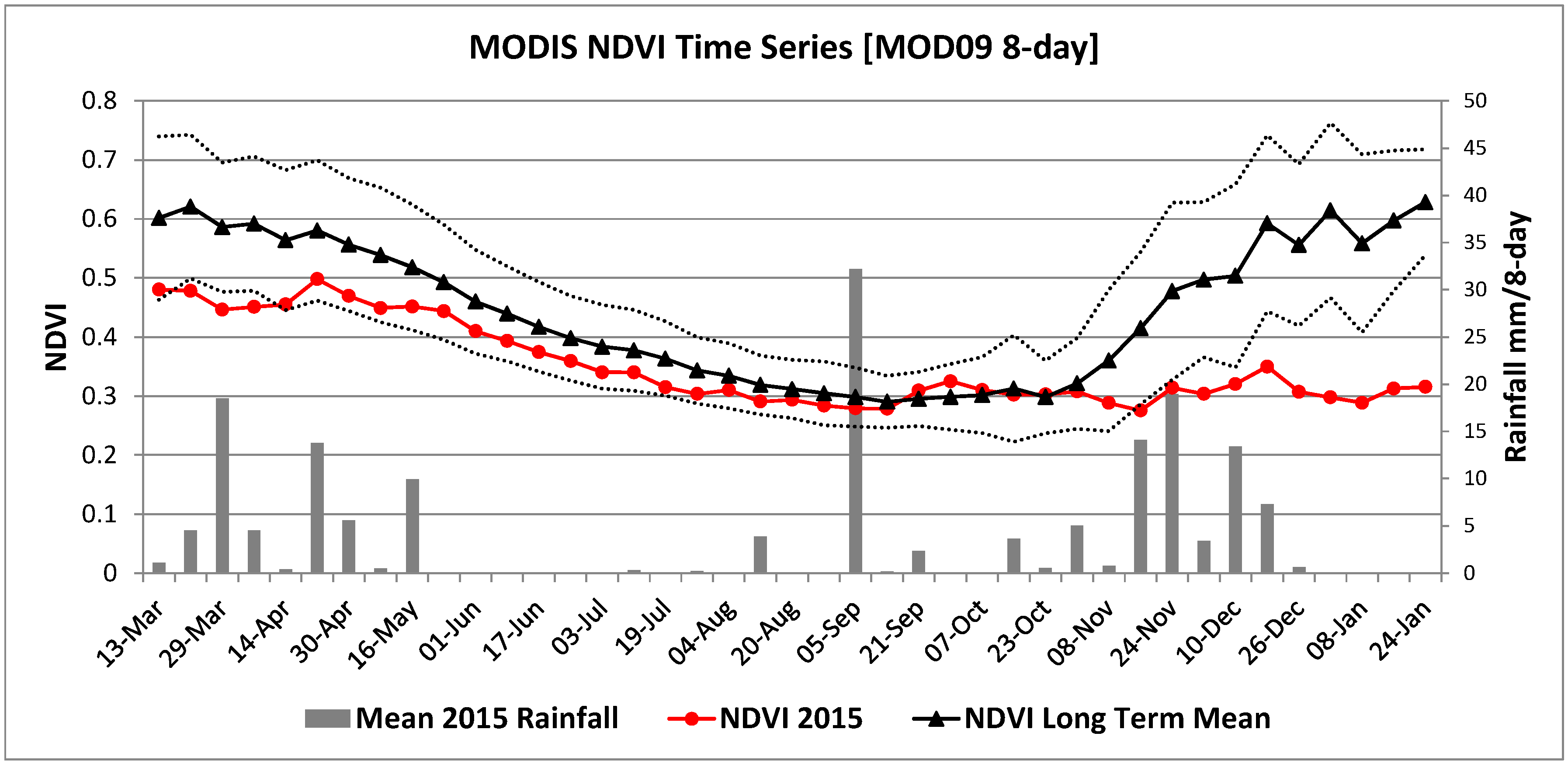
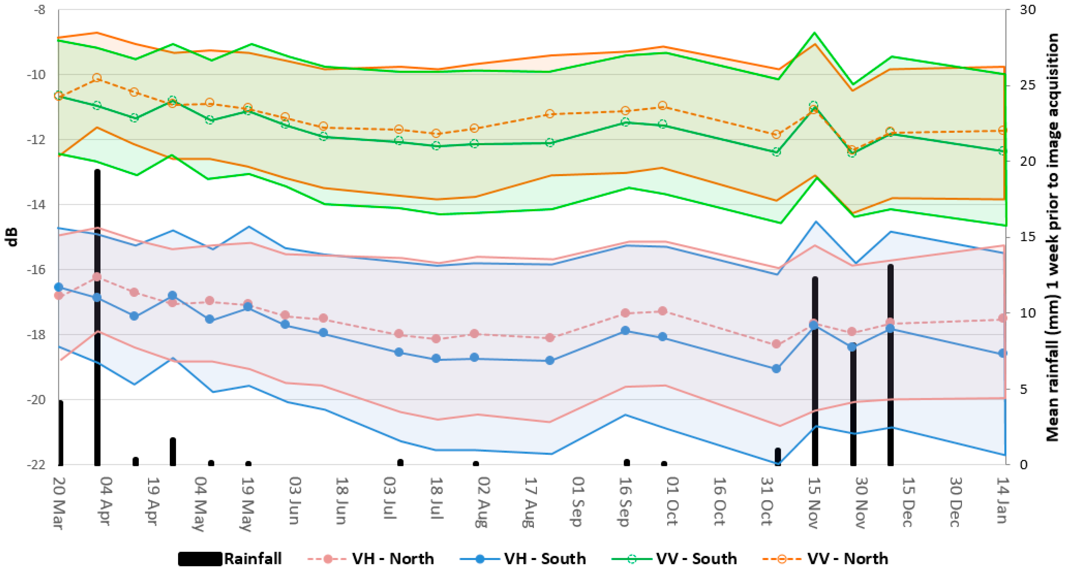
3.1. Backscatter and Environmental Temporal Dynamics

The long-term (2000–2015) MODIS NDVI, 2015 MODIS NDVI, and 2015 rainfall data for the park are shown in Figure 5. The long-term MODIS NDVI reflects the well-known phenological cycle characterizing southern African savannahs. Vegetation starts greening at the end of October with the first rains, to reach a maximum between January and March in the middle of the wet season. From April onwards the landscape dries up—grasses senesce and woody plants (mostly deciduous) shed their leaves—and the NDVI reaches a minimum in early September before the new rains of the following cycle. In 2015, the NDVI greening profile was below the long-term mean for most of the year. In November–December, the NDVI remained low because the first rains arrived late (mid-November instead of mid-October), and these were interrupted by an exceptional El Niño southern oscillation (ENSO) event. The regional 2015–2016 cycle experienced well below-average rainfall and an intense drought [84]. Early rainfall from mid-October to early December resulted in a slight NDVI increase (from 0.28 to 0.35), mostly in the wetter southern section of the park, which then collapsed well below the one standard deviation long-term mean line when the drought started in early December. The wet season of the previous cycle 2014–2015 already experienced below average NDVI, also as result of a low rainfall (Figure 5). Interestingly, several large rainfall events in August and early September resulted in a brief episode of NDVI increase.
The mean Sentinel-1 VV and VH backscatter data computed for the northern (>24°S) and southern (<24°S) sections of the KNP are shown in Figure 6, with the mean total rainfall data for the seven days prior to each Sentinel-1 image acquisition. The mean 2015 backscatter profile generally follows the rainfall and NDVI greening patterns; for example, the decreasing backscatter trend from April to July corresponds with the senescing/drying periods captured in the 2015 NDVI decreasing trend (Figure 5). After the month of October, the backscatter does not increase significantly despite the early season rainfalls in November, indicating the start of the drought conditions. Overall, across the study timeframe, the backscatter range of variation was quite limited with a range of only 2 dB in both polarizations, in accordance with the drier conditions shown in the 2015 NDVI dynamic.

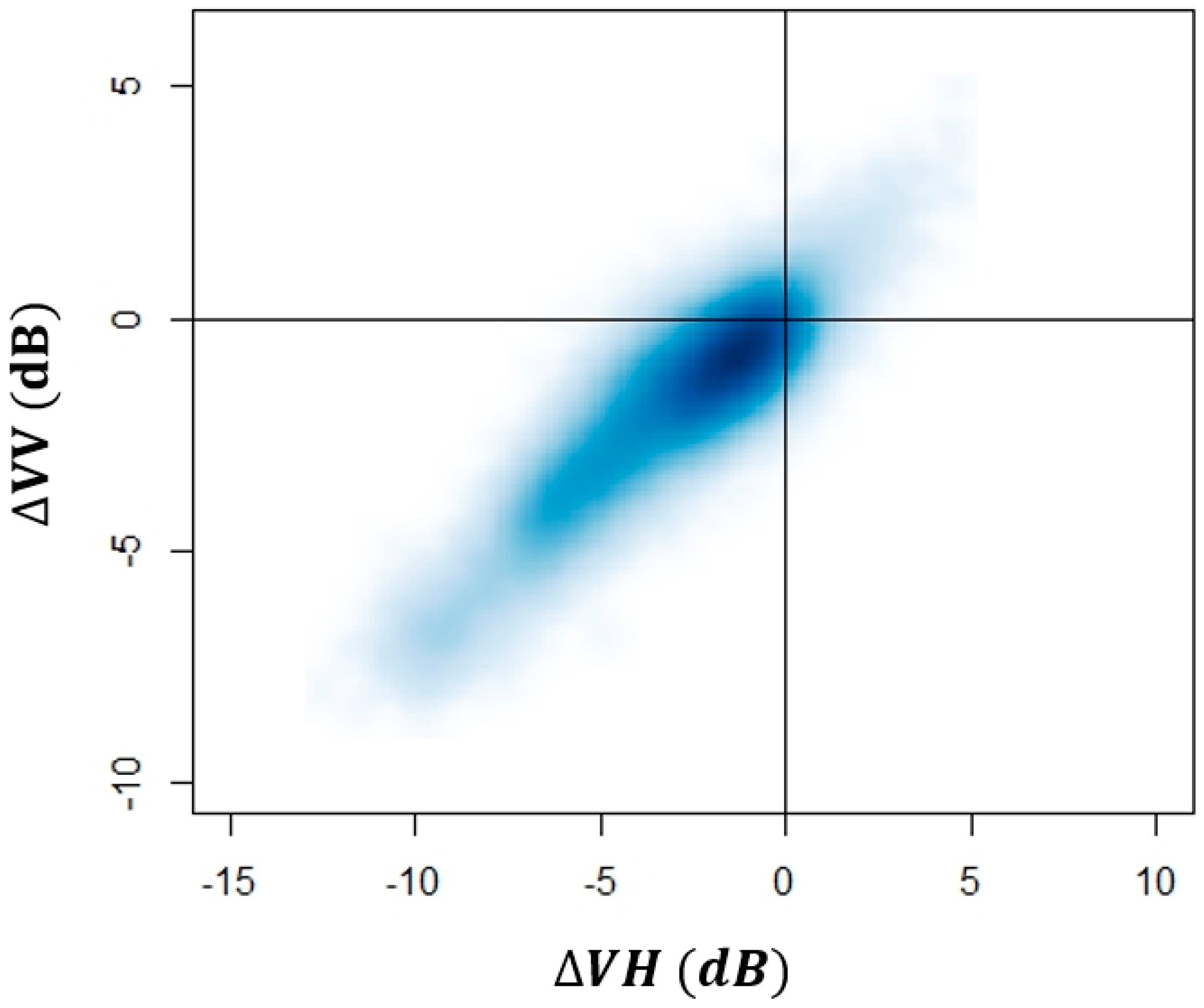
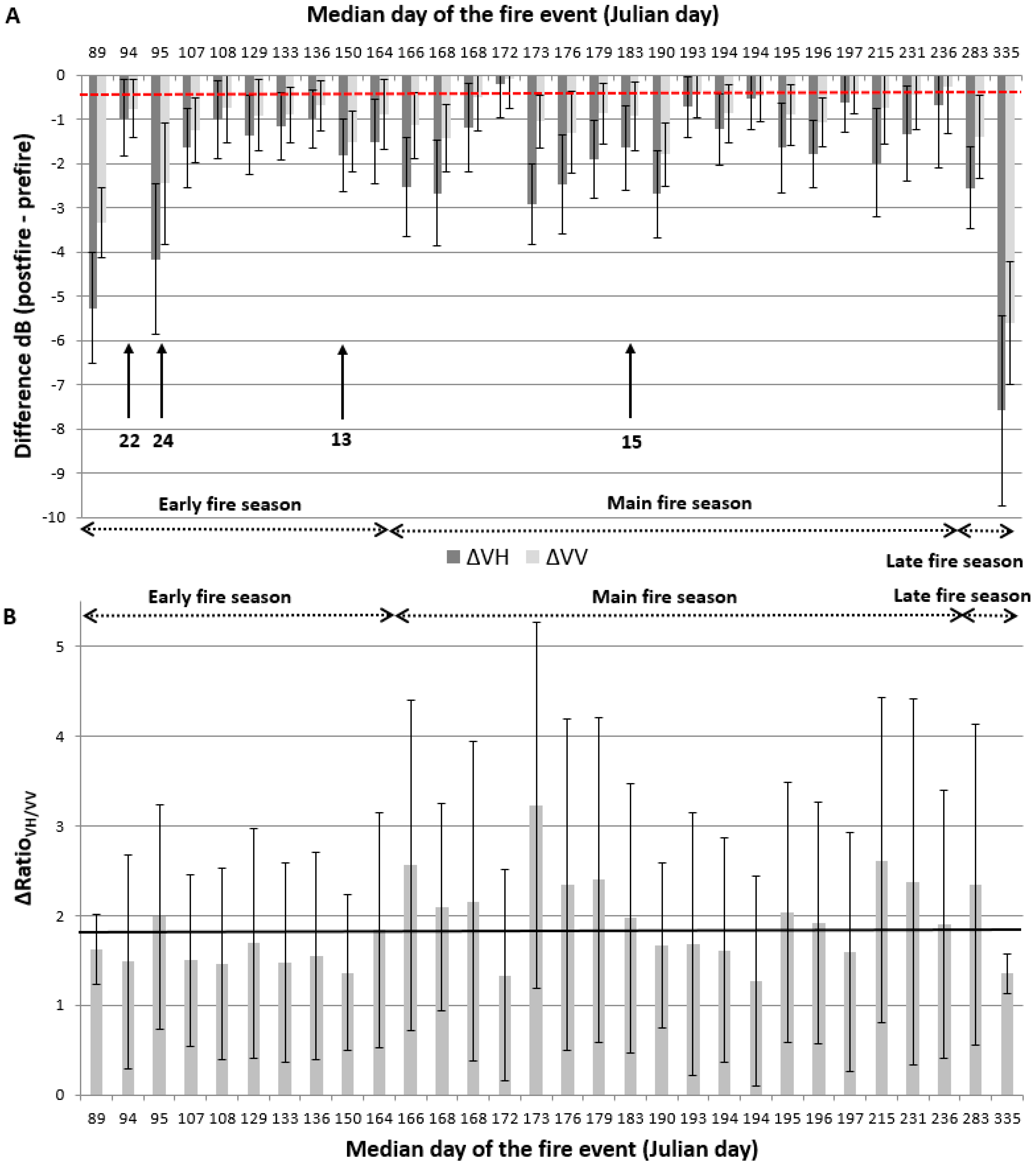
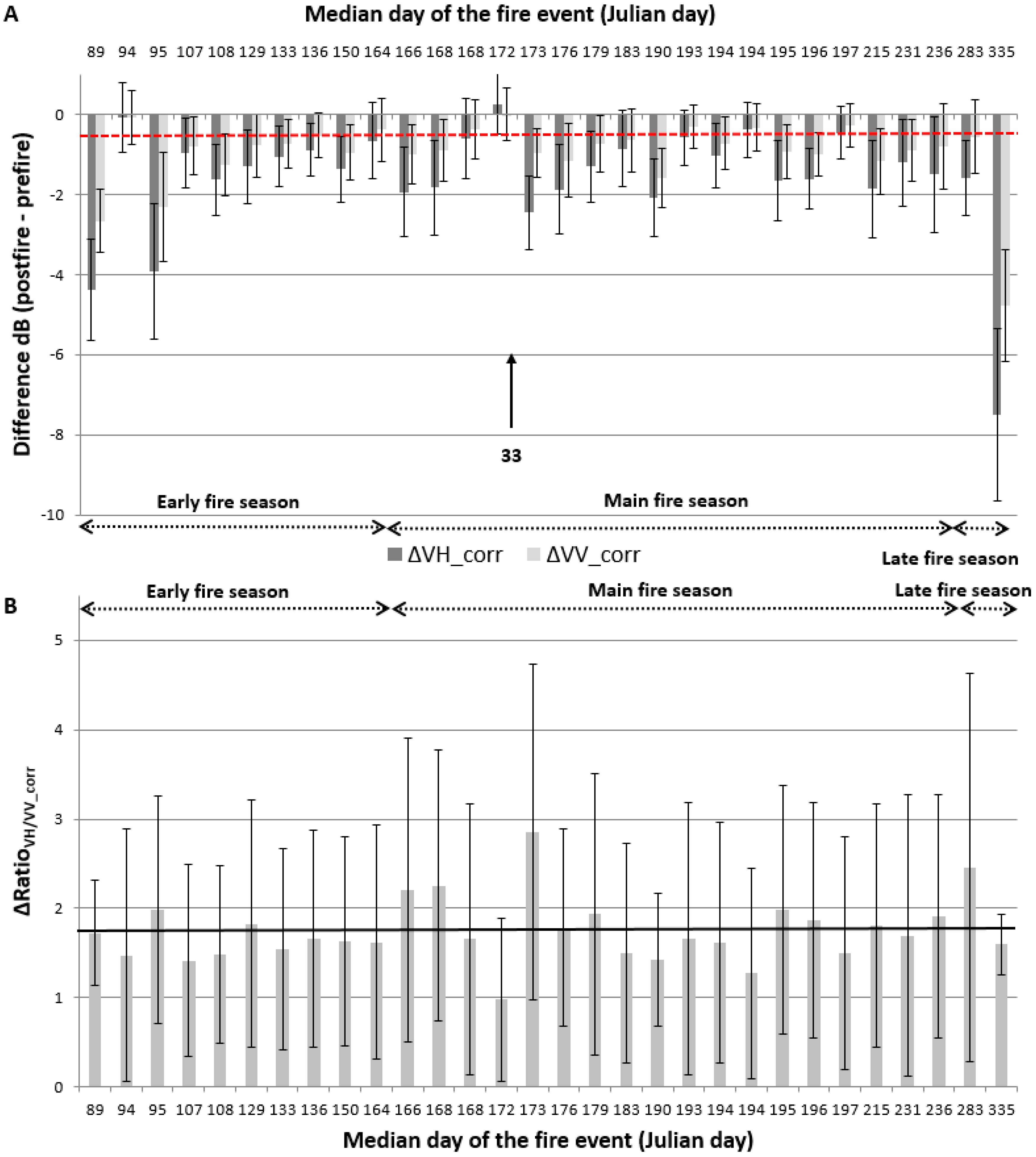
3.2. Pre-Fire Versus Post-Fire Backscatter Changes

Figure 7 shows the variability of pre-fire to post-fire backscatter differences Δ V V and Δ V H for all 100 m burn records (N = 106,000) measured in the 30 KNP burn events in 2015. The mean difference was a backscatter decrease of 2.36 dB (standard deviation STD = 2.01 dB) and 1.45 dB (STD = 1.41 dB), in the VH and VV polarizations, respectively. From the total 106,000 pixels, 2.95% exhibited a positive change in VH and VV (mean = 0.72 dB and STD = 0.74 dB, mean = 0.69 dB and STD = 0.64 dB for VH and VV, respectively), 3.18% a positive change in VH and a negative change in VV (mean = 0.35 dB and STD = 0.31 dB, mean = −0.52 dB and STD = 0.4 dB for VH and VV, respectively), 7.2% a negative change in VH and a positive change in VV (mean = −0.95 dB and STD = 0.71 dB, mean = 0.33 dB and STD = 0.3 dB for VH and VV, respectively), and 86.7% a negative change in VH and VV (mean = −2.68 dB and STD = 1.93 dB, mean = −1.70 dB and STD = 1.33 dB for VH and VV, respectively).
The mean backscatter differences between the post-fire and pre-fire images for each of the 30 burn events are shown in Figure 8. All of the burn events exhibit a mean post-fire backscatter decrease in both polarizations, with greater VH than VV decreases (Figure 8A). The mean backscatter decrease considering all 30 burn events was −1.96 dB (STD = 1.0 dB) for the VH polarization and −1.17 dB (STD = 0.76 dB) for the VV polarization. A total of 29 (96.7%) and 27 (90%) burn events had a decrease in VH and VV backscatter greater than 0.43 dB, the overall absolute radiometric accuracy of the Sentinel-1A products [68]. This value provides a general reference against which the significance of the Sentinel-1 backscatter change can be assessed, i.e., a change below 0.43 dB may not result from a target change on the ground. In addition, a Wilcoxon signed-rank test showed a significant difference between the pre-fire and post-fire backscatter value (p-value < 0.01 for both polarization VH and VV). We calculated the ratio Δ r a t i o V H / V V to compare the relative effect of fire on the backscatter of both polarizations. We only included pixels that exhibited a backscatter decrease in both polarizations, as this was the main observed dynamic in the burnt areas. In addition, we further discarded pixels that had a backscatter decrease below 0.2 dB in the VV polarization since low backscatter change values tended to generate an abnormally high ratio. The mean ratio of the VH and VV difference (Figure 8B) was always ≥1.2 and over the 30 burn events, had a mean of 1.9 (STD 1.33), indicating that the cross-polarized Sentinel-1 band (VH) is close to being twice as sensitive to fire-induced changes as the co-polarized (VV) band. When considering the results by fire season, the largest backscatter decreases for both polarizations were observed in the late season (N = 2, mean = −5.06 and −3.50 dB with also the highest STD, 3.56 and 2.97dB for VH and VV, respectively) and then in the early season (N = 9, mean = −2.04 and −1.39 dB with 1.56 and 0.91dB STD for VH and VV, respectively). In the main fire season, i.e., the driest months between June and September, intermediate decreases (N = 19, mean = −1.59 and −0.82dB with the lowest 0.82 and 0.43 dB STD for VH and VV, respectively) were observed. The Wilcoxon signed-rank test was significant for the early fire season (p-value = 0.03 and 0.05 for VH and VV, respectively) and the main fire season (p-value = 0.02 and 0.05 for VH and VV, respectively), but not significant for the late fire season, which, in 2015, included only two fires (p-value = 0.67 and 0.33 for VH and VV, respectively).
Figure 9 shows the same results as Figure 8 but considering the differences derived with the regional correction factors (Equations (6)–(8)) to reduce non-fire-related environmental changes occurring between the pre-fire and post-fire images, such as woody plant leaf shedding or display, and changes in soil and vegetation moisture. All of the burn events (except one, burn event 33) still exhibited a post-fire backscatter decrease in both polarizations (Figure 9A). A total of 27 (90%) and 23 (75%) burn events showed a decrease in VH and VV backscatter greater than 0.43 dB. The mean backscatter decrease for all fires was reduced by 0.35 dB to −1.61 dB (STD 1.0 dB), and by 0.2 dB to -0.99 dB (STD 0.77 dB) for the VH and VV polarizations, respectively. This indicates the overall drying conditions during the fire season. Again, the Wilcoxon signed-rank test showed a significant difference between the pre-fire and post-fire backscatter value (p-value < 0.01 for both polarization VH and VV). The mean ΔRatioVH/VV_corr (Figure 9B) was generally ≥1.0, except for the fire event 33, which showed a pre-fire to post-fire increase of VH backscatter. The ratios of the VH and VV difference (Figure 9B, mean 1.7, STD 0.78) were similar to the uncorrected ratios (Figure 8B). When examining the results by fire season, the results were similar than in the previous section, with the largest backscatter decreases observed in the late season (N = 2, −4.54 and −2.66 dB with also the highest STD, 4.17 and 2.98 dB for VH and VV, respectively), followed by the early season (N = 9, −1.73 and −1.12dB with 1.43 and 0.83 dB STD for VH and VV, respectively), and the main fire season (N = 19, −1.24 and -0.75 dB with the lowest 0.71 and 0.39 dB STD for VH and VV, respectively). The Wilcoxon signed-rank test was significant for the early fire season (p-value = 0.07 and 0.06 for VH and VV, respectively) and the main fire season (p-value = 0.03 and 0.05 for VH and VV, respectively), but again, not significant for the late fire season (p-value = 0.67 and 0.67 for VH and VV, respectively).

3.3. Relationships between Pre-Fire Versus Post-Fire Backscatter Changes and Rainfall

Most fires occur during dry periods—90% of the fires occur between mid-May and mid-September when only 5% of the total rain fell in the region. Due to the importance of surface moisture conditions on radar scattering, we sought to verify the potential effect of rainfall on the backscatter changes between the pre-fire and post-fire images. The total rainfall before the acquisition of each Sentinel-1A image (pre- and post-fire) is an indicator of the possible confounding effects of surface moisture on the backscatter. We hypothesized that ground fires in savannahs decrease the C-band backscatter because of the burning and physical removal of dry grasses and vegetation debris. However, a rainfall event prior to the pre-fire image would increase the Δ V V and Δ V H backscatter decrease (by increasing the pre-fire image backscatter), whereas a rainfall event prior to the post-fire image would tend to reduce the Δ V V and Δ V H backscatter decrease (increasing the post-fire image backscatter). A similar amount of rainfall prior to both dates is likely to balance each other out and have a null effect on the backscatter difference; although this assumes a similar effect of moisture on the backscatter of a grass layer and bare ground. We, thus, calculated the total rainfall prior to the post-fire image minus total rainfall prior to the pre-fire image (RDIFF) and regressed it against Δ V V and Δ V H . Positive rainfall values indicate higher rainfall during the day(s) prior to the pre-fire image compared to the day(s) prior to the post-fire image, and negative rainfall values indicate higher rainfall during the day(s) prior to the post-fire image. A high dependence of Δ V H and Δ V V backscatter changes on rainfall is expected to exhibit a significant negative relationship. The rainfall data (mm) for each burn event were derived from the closest weather station. The mean distance weather station to burn event was 12 km. The possible effect of rainfall over seven, five, three, and one days before the Sentinel-1A acquisition dates (Table 1) were examined. Given the dry conditions and high infiltration and evaporation rates in the region, it is unlikely that rainfall would have an influence beyond seven days.
The relationships between Δ V H and Δ V V and RDIFF were not significant for the scenarios where rainfall was measured one, five, and seven days prior to the image acquisitions for both polarizations (R2 ~ 0.03–0.001). For the three-day scenario, the relationships were negatively correlated (R2 ~ 0.33–0.2), but were only significant (p < 0.01) for the VV polarization (Table 1). This result is driven by one burn event, which was affected by a 10 mm rainfall event three days prior to the pre-fire image during the late fire season. SAR imagery is known to be sensitive to surface moisture. However, the period under investigation corresponds to the dry season in Southern Africa, when most fires burn and when rainfall events are uncommon. From the 30 fire events recorded in KNP, 19 did not receive any rainfall seven days prior to the pre- or post-fire Sentinel-1A image acquisition, and only three burn events received more than 5 mm of rainfall seven days prior to the pre- or post-fire Sentinel-1A image acquisition. Overall, the results indicate that for 2015, rainfall had limited effect on the backscatter changes. If we could not find evident moisture effects on backscatter change over the burn events, it cannot be ruled out that moisture effects might be potentially higher in a wetter year.

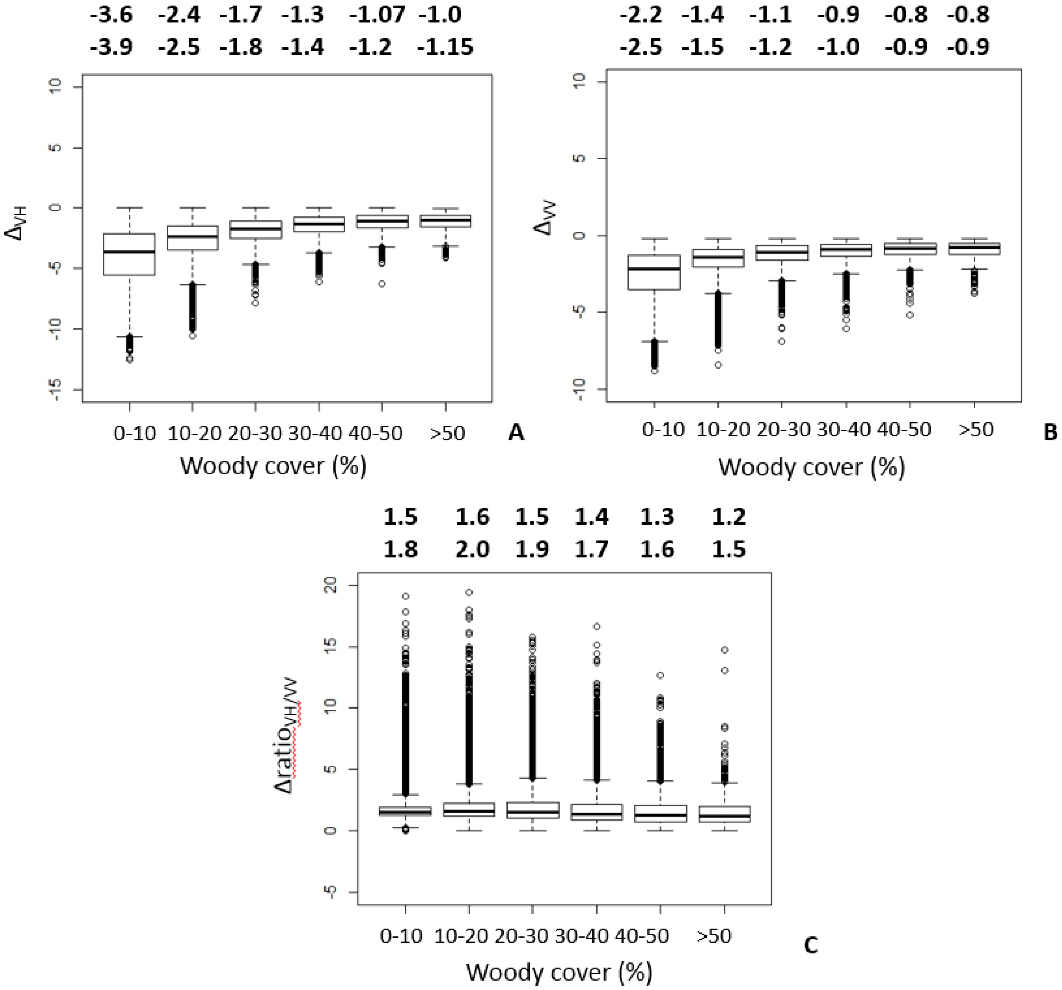
3.4. Effect of Woody Cover

Figure 10 shows examples of Sentinel-1A images over burned areas in grasslands and in woodier savannah KNP landscapes. All the burned areas are clearly visible within their surroundings and match the Landsat burned areas (red outlines) quite well. The contrast between non-burned and burned regions is less evident in the woody-dominated landscapes than in the grassland-dominated landscapes. Burn event 22 is a good example where the fire propagated through a granitic area with a woody canopy cover around 30%–40% to the north and an area intruded by gabbro sills with a woody canopy cover around 5%–15% in the south. The boundary between the two geological formations is very evident and suggests a stronger effect of fire on the C-band backscatter dynamics in grasslands, or more spatially fragmented and/or less complete combustion in the woodland area.
The backscatter differences in individual 1 ha pixels were compared with the corresponding woody cover for all the burn events in Figure 11. The woody cover was quantized into 10% intervals, with just one class representing woody cover ≥50%. For both polarizations (Figure 11A,B), greater woody cover is associated with smaller pre-fire and post-fire backscatter change, with reduced within-cover class variability. Fire effects on backscatter were higher for the VH than the VV polarization, but this effect was reduced at higher woody cover. The woody cover effect on backscatter change tended to saturate above about 30% cover. The Δ r a t i o V H / V V was around 1.5 for the lowest woody cover class and tended to decrease with an increasing woody cover, to reach a ratio below one for the woody cover classes above 40%. This later result means that the VV polarization is slightly more sensitive to fire-driven backscatter changes than the VH polarization when the woody cover is denser (Figure 11C). Similar results were found when the regionally corrected backscatter differences (Equations (6)–(8)) were considered (not shown). A Kruskal–Wallis (H-test) was conducted, which showed that there were significant differences (i.e., H statistic > χ2 critical value) in Δ V H , Δ V V , and Δ r a t i o V H / V V differences between the woody cover intervals (N = 106,000+, H = 24,546, 29,223, 1145 with χ2 critical value 11.07, for Δ V H , Δ V V , and Δ r a t i o V H / V V , respectively).

4. Discussion

A number of environmental factors may have influenced the SAR backscatter reported in this study and are potential confounding factors for the detection of burned areas. These include changes in soil and vegetation moisture content, and changes in phenology of the two main life forms, grasses, and woody plants. Moisture is present in various forms across KNP with variable persistence. Dew can form at night, even in the dry season, and so may increase the backscatter of images acquired in the early morning compared to those acquired in the afternoon. In the current study, however, all the Sentinel-1 images were acquired in the afternoon. Rainfall infiltrates the soil layer, then evaporates or is taken up by plants for growth, and across KNP, this mostly occurs as discrete events associated with short-duration convective thunderstorms [60]. Grass greening and senescence is in response to rainfall but with high inter-annual temporal and spatial variability depending on the timing and amplitude of the rainfall events [82]. From April to June (wet to dry transition season) or from September to October (dry to wet transition season), the backscatter is also influenced by the shedding or display of tree canopy leaves (most KNP savanna species are deciduous). Leaf display or shedding is spatially and temporally more homogeneous than grass greening or senescence [82]. Leaf display occurs generally before the first rains between the end of September and mid-October. However, tree species and water availability through soil type or landscape position influence spatial variability of tree phenology [82,85,86].
The gradual Sentinel-1A backscatter decrease (−2 dB) observed from the beginning of April to early July (Figure 6) is most likely indicative of a general drying across the landscape. After this date, the backscatter stabilized to its lowest level until early September. The shedding of leaves may have impacted this pattern. The effect of leaves on SAR backscatter can be complex as they influence the penetration depth of microwaves, and their interactions with the canopy and underlying layers. For short microwaves, leaves tend to act as scatterers and attenuators, while for long microwaves, they act mostly as attenuators [67]. Thus, an increase in tree canopy leaf area index (LAI) has been associated with an increase in X-band backscatter [87], while leaf-off scenarios have been observed to increase the L-band backscatter—due to a higher penetration of microwave in the canopy and interaction with the ground and trunk—compared to leaf-on scenarios [67]. Published data are limited in savannahs. Positive correlations established between tree foliage biomass and C-band backscatter in Australia [88,89] suggest that leaf shedding would contribute to further decrease the Sentinel-1 backscatter. In addition, the decrease in foliage elements due to fires resulted in decreased C-band cross-polarized backscatter by about 2–3 dB over dry Mediterranean forests, but it increased in the co-polarized frequencies [42]. Studies are recommended to better understand the effect of leaf-on versus leaf-off on the backscatter, considering the specificities of trees found in savannahs, e.g., broad versus fine leaves species, and low LAI.
For the KNP 30 burn events, a systematic decrease of the SAR backscatter from pre-fire to post-fire was observed with a mean backscatter decrease of −1.61 dB and −0.99 dB for the VH and VV polarizations, respectively. The cross-polarization VH data were found to be nearly twice as sensitive to fire as the VV co-polarization data (Figure 8 and Figure 9). The large ratio VH/VV values, consistent across fire events and seasons, suggest that the dominant fire effect detected by pre-fire and post-fire backscatter change is linked to the removal of grass and a decrease in C-band volume scattering, which has been observed in other studies [40]. However, the decrease of the ratio VH/VV with the woody cover (Figure 11C), below one when the woody cover is above 40%, may indicate an increase of the cross-polarized signal interaction with the woody layer.
The early season fires produced greater backscatter decreases compared to main season fires. During the early fire season, the landscape is in a drying phase with a decrease of grass and soil moisture (see NDVI and backscatter profiles in Figure 5 and Figure 6). Although early season fires are expected to be less intense, and possibly less complete than main season fires [63], the grass removal by early season fires could have several effects, namely (i) removal of grass scatterers, (ii) decrease in grass moisture, and (iii) decrease of soil moisture due to fire [53]. Moisture changes were at their minimum during July–August (Figure 6), so this suggests that the backscatter changes during the main fire season are likely a result of the removal of grass scatterers and a corresponding decrease in volume scattering, while early fire season backscatter changes resulted from both changes in grass scatterers and moisture. Difference of pre-fire grass conditions, including biomass and grass communities with varying plant height, leaf structure, and shape, may explain the large variability of Δ V H and Δ V V backscatter observed at low woody cover (0%–20%, Figure 11), over 3 and 2 dB for the VH and VV polarizations, respectively. Grass biomass is mostly controlled by rainfall and soil fertility, but is also linked to the time elapsed since the last burn, since grass biomass accumulates from one year to another without fire [63]. Higher pre-fire grass biomass would lead to a higher backscatter decrease after a burn event. In addition, fire removes and changes the vegetation structure and may reveal the underlying soil [26,90]. Different soils and bare ground conditions may influence the variability of fire-induced changes on backscatter changes. The post-fire image will have a higher soil background contribution, which could be affected by variable soil roughness, texture, and stoniness.
The magnitude of backscatter decrease due to fire is influenced by woody cover (Figure 11). Similar observations were reported with airborne C-band SAR data over a burned area in a tropical Australian savannah [53]. High woody cover is associated with lower grass biomass due to resource competition, e.g., water, sunlight [17], and is likely to produce less intense or frequent fires, possibly with a less complete combustion of the grass layer. In addition, a higher woody canopy cover reduces gaps and increases the attenuation of microwaves travelling through the canopies, especially with leaf-on scenarios [91], therefore it reduces the signal reaching and interacting with the ground where most of the fire effects in savannahs occur, through the removal of grasses and debris. Although fire is an important driver of long-term woody structure in African savannahs [13,92], backscatter change attributed to tree damages is limited (see for instance the small backscatter decrease shown in dense woodlands −0.55 dB for VH and −0.31 dB for VV, below the Sentinel-1 radiometric accuracy for the latter, Figure 11A,B). Savannah fires are primarily ground fires of lower intensity than canopy fires occurring in denser forests [52]. Woody savannah species have developed fire-resistant mechanisms, e.g., thick and/or corky bark, rapid early growth, and vigorous resprouting [51,93]; thus, savannah fires rarely affect large trees except when they have been previously weakened by animal or insect damage [62,94]. Damages in the shrubby strata may occur, but would also lead to a decrease of backscatter, enhancing the detectability of burned patches. A woody cover above 30%–40% might act as a buffer layer for the microwaves and might be more challenging to detect burned areas with C-band SAR.

5. Conclusions

The effect of surface fires in southern African deciduous savannahs on the backscatter of multi-temporal C-band SAR Sentinel-1A data was investigated. We hypothesized that C-band backscatter would be affected by the removal of grass scatterers in surface fires in savannahs, and that the C-band VH backscatter would be more sensitive than the VV backscatter. For 30 burn events in the KNP, we observed a systematic pre-fire to post-fire decrease of backscatter (mean of −1.61 dB and −0.99 dB for the VH and VV polarizations) considering the 18 Sentinel-1A C-band images acquired between 20 March and 9 December 2015. Between 90% and 75% of the burn events had a backscatter decrease greater than the Sentinel-1 radiometric accuracy (0.43 dB), for VH and VV, respectively. The cross-polarization VH was nearly twice as sensitive to fire-induced changes as the co-polarization VV data. Pre-fire and post-fire backscatter changes most likely resulted from a reduction in grass biomass and moisture levels. Early season fires produced higher decreases compared to the main season fires, possibly due to greater fire-induced moisture changes (e.g., removal of grasses with higher moisture content). Over 30% woody cover the fire effects on the backscatter of the C-band Sentinel-1 images were reduced, with a lower decrease of backscatter values between pre- and post-fire conditions. Denser woody communities tend to produce lower grass fuel load and less intense surface fires, and limit the penetration of C-band microwaves to the ground where most savannah fires occur.
This research provides evidence that C-band spaceborne SAR is sensitive to surface fire effects in southern African deciduous savannahs. Additional research will be required to assess how these results can be used possibly to develop a burnt areas detection algorithm based on Sentinel-1 data, to extract burnt patches, and assess burnt areas detection rates. Important limitations exist in densely wooded areas. However, the availability of high temporal C-band datasets from the Sentinel-1 SAR constellation (six-day revisit) suggest that this technology can play a greater role in burned area mapping and monitoring, in particular in combination with optical wavelength moderate resolution Landsat-8 and Sentinel-2 data that have good burned area discrimination [95] but unlike SAR, cannot work under cloudy conditions. This may open up opportunities for fine-scale fire propagation studies and a better understanding of fire processes and drivers. In 2018, for example, both Sentinel-1 platforms acquired SAR images in the KNP region in average every eight days.

Author Contributions

Conceptualization, R.M. (Renaud Mathieu) and, R.M. (Russell Main); methodology, R.M. (Renaud Mathieu), R.M. (Russell Main), and L.N.; formal analysis, R.M. (Renaud Mathieu), D.R., R.M. (Russell Main), and L.N.; data curation and processing, R.M. (Russell Main), H.Y., and L.N.; writing—original draft preparation, R.M. (Renaud Mathieu); writing—review and editing, D.R.

Funding

This research was undertaken with funding provided by the Council of Science and Industrial Research (CSIR), South Africa: NRE Parliamentary Grant “Multi-Domain Development Platform (CMDP) to Realize National Value of the Sentinel Sensors for various land, fresh water and marine societal benefit areas”, and Thematic Programme 45 “National woody vegetation monitoring system for ecosystem and value-added services”.

Acknowledgments

The European Space Agency (ESA) and Copernicus program management and staff are thanked for the free provision of the Sentinel-1 data. The USGS Landsat program management and staff, are thanked for the free provision of the Landsat data. CSIR-Meraka and NASA are thanked for the provision of the MODIS burned area products. We also acknowledge the use of data and imagery from LANCE FIRMS operated by the NASA/GSFC/Earth Science Data and Information System (ESDIS) with funding provided by NASA/HQ.

Conflicts of Interest

The authors declare no conflict of interest. The funders had no role in the design of the study; in the collection, analyses, or interpretation of data; in the writing of the manuscript, or in the decision to publish the results.

References

  1. Chuvieco, E.; Yue, C.; Heil, A.; Mouillot, F.; Alonso-Canas, I.; Padilla, M.; Pereira, J.M.; Oom, D.; Tansey, K. A New Global Burned Area Product for Climate Assessment of Fire Impacts. Glob. Ecol. Biogeogr. 2016, 25, 619–629. [Google Scholar] [CrossRef]
  2. Roy, D.P.; Boschetti, L.; Justice, C.O.; Ju, J. The Collection 5 MODIS Burned Area Product—Global Evaluation by Comparison with the MODIS Active Fire Product. Remote Sens. Environ. 2008, 112, 3690–3707. [Google Scholar] [CrossRef]
  3. van der Werf, G.R.; Randerson, J.T.; Giglio, L.; Collatz, G.J.; Mu, M.; Kasibhatla, P.S.; Morton, D.C.; DeFries, R.S.; Jin, Y.; van Leeuwen, T.T. Global Fire Emissions and the Contribution of Deforestation, Savanna, Forest, Agricultural, and Peat Fires (1997–2009). Atmos. Chem. Phys. Discuss. 2010, 10, 11707–11735. [Google Scholar] [CrossRef]
  4. Bond, W.J.; Keeley, J.E. Fire as a Global ‘Herbivore’: The Ecology and Evolution of Flammable Ecosystems. Trends Ecol. Evol. 2005, 20, 387–394. [Google Scholar] [CrossRef]
  5. Archibald, S.; Scholes, R.J.; Roy, D.P.; Roberts, G.; Boschetti, L. Southern African Fire Regimes as Revealed by Remote Sensing. Int. J. Wildland Fire 2010, 19, 861–878. [Google Scholar] [CrossRef]
  6. Sheuyange, A.; Oba, G.; Weladji, R.B. Effects of Anthropogenic Fire History on Savanna Vegetation in Northeastern Namibia. J. Environ. Manag. 2005, 75, 189–198. [Google Scholar] [CrossRef] [PubMed]
  7. Mapiye, C.; Chikumba, N.; Chimonyo, M.; Mwale, M. Fire as a Rangeland Management Tool in the Savannas of Southern Africa: A Review. Trop. Subtrop. Agroecosyst. 2008, 8, 115–124. [Google Scholar]
  8. Lohmann, D.; Tietjen, B.; Blaum, N.; Joubert, D.F.; Jeltsch, F. Prescribed Fire as a Tool for Managing Shrub Encroachment in Semi-Arid Savanna Rangelands. J. Arid Environ. 2014, 107, 49–56. [Google Scholar] [CrossRef]
  9. Frost, P.G.H. Fire in southern African woodlands: Origins, impacts, effects, and control. In Proceedings of the FAO Meeting on Public Policies Affecting Forest Fires, FAO Forestry Paper 138. Rome, Italy, 28–30 October 1998; FAO; pp. 181–205. [Google Scholar]
  10. Jin, Y.; Roy, D.P. Fire-Induced Albedo Change and its Radiative Forcing at the Surface in Northern Australia. Geophys. Res. Lett. 2005, 32, L13401. [Google Scholar] [CrossRef]
  11. Levick, S.R.; Asner, G.P.; Smit, I.P.J. Spatial Patterns in the Effects of Fire on Savanna Vegetation Three-Dimensional Structure. Ecol. Appl. 2012, 22, 2110–2121. [Google Scholar] [CrossRef]
  12. Moreira, A.G. Effects of Fire Protection on Savanna Structure in Central Brazil. J. Biogeogr. 2000, 27, 1021–1029. [Google Scholar] [CrossRef]
  13. Smit, I.P.J.; Asner, G.P.; Govender, N.; Kennedy-Bowdoin, T.; Knapp, D.E.; Jacobson, J. Effects of Fire on Woody Vegetation Structure in African Savanna. Ecol. Appl. 2010, 20, 1865–1875. [Google Scholar] [CrossRef] [PubMed]
  14. Andersen, A.N.; Woinarski, J.C.Z.; Parr, C.L. Savanna Burning for Biodiversity: Fire Management for Faunal Conservation in Australian Tropical Savannas. Austral Ecol. 2012, 37, 658–667. [Google Scholar] [CrossRef]
  15. Medina, E.; Silva, J.F. Savannas of Northern South-America—A Steady-State Regulated by Water Fire Interactions on a Background of Low Nutrient Availability. J. Biogeogr. 1990, 17, 403–413. [Google Scholar] [CrossRef]
  16. Oba, G.; Post, E.; Syvertsen, P.O.; Stenseth, N.C. Bush Cover and Range Condition Assessments in Relation to Landscape and Grazing in Southern Ethiopia. Landsc. Ecol. 2000, 15, 535–546. [Google Scholar] [CrossRef]
  17. Smit, I.P.J.; Prins, H.H.T. Predicting the Effects of Woody Encroachment on Mammal Communities, Grazing Biomass and Fire Frequency in African Savannas. PLoS ONE 2015, 10, e0137857. [Google Scholar] [CrossRef] [PubMed]
  18. Jain, A.K. Global Estimation of CO Emissions using Three Sets of Satellite Data for Burned Area. Atmos. Environ. 2007, 41, 6931–6940. [Google Scholar] [CrossRef]
  19. Stroppiana, D.; Brivio, P.A.; Gregoire, J.M.; Liousse, C.; Guillaume, B.; Granier, C.; Mieville, A.; Chin, M.; Petron, G. Comparison of Global Inventories of CO Emissions from Biomass Burning Derived from Remotely Sensed Data. Atmos. Chem. Phys. 2010, 10, 12173–12189. [Google Scholar] [CrossRef]
  20. Williams, J.E.; van Weele, M.; van Velthoven, P.F.J.; Scheele, M.P.; Liousse, C.; van der Werf, G.R. The Impact of Uncertainties in African Biomass Burning Emission Estimates on Modeling Global Air Quality, Long Range Transport and Tropospheric Chemical Lifetimes. Atmosphere 2012, 3, 132–163. [Google Scholar] [CrossRef] [Green Version]
  21. Alvarado, S.T.; Fornazari, T.; Costola, A.; Morellato, L.P.C.; Silva, T.S.F. Drivers of Fire Occurrence in a Mountainous Brazilian Cerrado Savanna: Tracking Long-Term Fire Regimes using Remote Sensing. Ecol. Ind. 2017, 78, 270–281. [Google Scholar] [CrossRef]
  22. Archibald, S.; Roy, D.P.; van Wilgen, B.W.; Scholes, R.J. What Limits Fire? an Examination of Drivers of Burnt Area in Southern Africa. Glob. Chang. Biol. 2009, 15, 613–630. [Google Scholar] [CrossRef]
  23. Curt, T.; Borgniet, L.; Ibanez, T.; Moron, V.; Hely, C. Understanding Fire Patterns and Fire Drivers for Setting a Sustainable Management Policy of the New-Caledonian Biodiversity Hotspot. For. Ecol. Manag. 2015, 337, 48–60. [Google Scholar] [CrossRef]
  24. Le Maitre, D.C.; Kruger, F.J.; Forsyth, G.G. Interfacing Ecology and Policy: Developing an Ecological Framework and Evidence Base to Support Wildfire Management in South Africa. Austral Ecol. 2014, 39, 424–436. [Google Scholar] [CrossRef]
  25. Trigg, S.N.; Roy, D.P. A Focus Group Study of Factors that Promote and Constrain the use of Satellite-Derived Fire Products by Resource Managers in Southern Africa. J. Environ. Manag. 2007, 82, 95–110. [Google Scholar] [CrossRef] [PubMed]
  26. Roy, D.; Landmann, T. Characterizing the Surface Heterogeneity of Fire Effects using Multi-Temporal Reflective Wavelength Data. Int. J. Remote Sens. 2005, 26, 4197–4218. [Google Scholar] [CrossRef]
  27. Mouillot, F.; Schultz, M.G.; Yue, C.; Cadule, P.; Tansey, K.; Ciais, P.; Chuvieco, E. Ten Years of Global Burned Area Products from Spaceborne Remote Sensing-A Review: Analysis of User Needs and Recommendations for Future Developments. Int. J. Appl. Earth Obs. Geoinf. 2014, 26, 64–79. [Google Scholar] [CrossRef]
  28. Ruiz, J.A.M.; Riano, D.; Arbelo, M.; French, N.H.F.; Ustin, S.L.; Whiting, M.L. Burned Area Mapping Time Series in Canada (1984-1999) from NOAA-AVHRR LTDR: A Comparison with Other Remote Sensing Products and Fire Perimeters. Remote Sens. Environ. 2012, 117, 407–414. [Google Scholar] [CrossRef]
  29. Giglio, L.; Boschetti, L.; Roy, D.P.; Humber, M.L.; Justice, C.O. The Collection 6 MODIS Burned Area Mapping Algorithm and Product. Remote Sens. Environ. 2018, 217, 72–85. [Google Scholar] [CrossRef]
  30. Tansey, K.; Gregoire, J.M.; Binaghi, E.; Boschetti, L.; Brivio, P.A.; Ershov, D.; Flasse, S.; Fraser, R.; Graetz, D.; Maggi, M.; et al. A Global Inventory of Burned Areas at 1km Resolution for the Year 2000 Derived from SPOT VEGETATION Data. Clim. Chang. 2004, 67, 345–377. [Google Scholar] [CrossRef]
  31. Boschetti, L.; Roy, D.P.; Justice, C.O.; Humber, M.L. MODIS-Landsat Fusion for Large Area 30 M Burned Area Mapping. Remote Sens. Environ. 2015, 161, 27–42. [Google Scholar] [CrossRef]
  32. Hawbaker, T.J.; Vanderhoof, M.K.; Beal, Y.J.; Takacs, J.D.; Schmidt, G.L.; Falgout, J.T.; Williams, B.; Fairaux, N.M.; Caldwell, M.K.; Picotte, J.J.; et al. Mapping Burned Areas using Dense Time-Series of Landsat Data. Remote Sens. Environ. 2017, 198, 504–522. [Google Scholar] [CrossRef]
  33. Siegert, F.; Ruecker, G.; Hinrichs, A.; Hoffmann, A.A. Increased Damage from Fires in Logged Forests during Droughts Caused by El Nino. Nature 2001, 414, 437–440. [Google Scholar] [CrossRef] [PubMed]
  34. Siegert, F.; Hoffmann, A.A. The 1998 Forest Fires in East Kalimantan (Indonesia): A Quantitative Evaluation using High Resolution, Multitemporal ERS-2 SAR Images and NOAA-AVHRR Hotspot Data. Remote Sens. Environ. 2000, 72, 64–77. [Google Scholar] [CrossRef]
  35. Verhegghen, A.; Eva, H.; Ceccherini, G.; Achard, F.; Gond, V.; Gourlet-Fleury, S.; Cerutti, P.O. The Potential of Sentinel Satellites for Burnt Area Mapping and Monitoring in the Congo Basin Forests. Remote Sens. 2016, 8, 986. [Google Scholar] [CrossRef]
  36. Bourgeau-Chavez, L.L.; Kasischke, E.S.; Brunzell, S.; Mudd, J.P.; Tukman, M. Mapping Fire Scars in Global Boreal Forests using Imaging Radar Data. Int. J. Remote Sens. 2002, 23, 4211–4234. [Google Scholar] [CrossRef]
  37. Huang, S.L.; Siegert, F. Backscatter Change on Fire Scars in Siberian Boreal Forests in ENVISAT ASAR Wide-Swath Images. IEEE Geosci. Remote Sens. Lett. 2006, 3, 154–158. [Google Scholar] [CrossRef]
  38. Rykhus, R.; Lu, Z. Monitoring a Boreal Wildfire using Multi-Temporal Radarsat-1 Intensity and Coherence Images. Geomat. Nat. Hazards Risk 2011, 2, 15–32. [Google Scholar] [CrossRef]
  39. Tanase, M.A.; Kennedy, R.; Aponte, C. Fire Severity Estimation from Space: A Comparison of Active and Passive Sensors and their Synergy for Different Forest Types. Int. J. Wildland Fire 2015, 24, 1062–1075. [Google Scholar] [CrossRef]
  40. Imperatore, P.; Azar, R.; Calo, F.; Stroppiana, D.; Brivio, P.A.; Lanari, R.; Pepe, A. Effect of the Vegetation Fire on Backscattering: An Investigation Based on Sentinel-1 Observations. IEEE J. Select. Top. Appl. Earth Obs. Remote Sens. 2017, 10, 4478–4492. [Google Scholar] [CrossRef]
  41. Polychronaki, A.; Gitas, I.Z.; Veraverbeke, S.; Debien, A. Evaluation of ALOS PALSAR Imagery for Burned Area Mapping in Greece using Object-Based Classification. Remote Sens. 2013, 5, 5680–5701. [Google Scholar] [CrossRef]
  42. Tanase, M.A.; Santoro, M.; de la Riva, J.; Perez-Cabello, F.; Le Toan, T. Sensitivity of X-, C-, and L-Band SAR Backscatter to Burn Severity in Mediterranean Pine Forests. IEEE Trans. Geosci. Remote Sens. 2010, 48, 3663–3675. [Google Scholar] [CrossRef]
  43. Minchella, A.; Del Frate, F.; Capogna, F.; Anselmi, S.; Manes, F. Use of Multitemporal SAR Data for Monitoring Vegetation Recovery of Mediterranean Burned Areas. Remote Sens. Environ. 2009, 113, 588–597. [Google Scholar] [CrossRef]
  44. Polychronaki, A.; Gitas, I.Z.; Minchella, A. Monitoring Post-Fire Vegetation Recovery in the Mediterranean using SPOT and ERS Imagery. Int. J. Wildland Fire 2014, 23, 631–642. [Google Scholar] [CrossRef]
  45. Tanase, M.; de la Riva, J.; Santoro, M.; Perez-Cabello, F.; Kasischke, E. Sensitivity of SAR Data to Post-Fire Forest Regrowth in Mediterranean and Boreal Forests. Remote Sens. Environ. 2011, 115, 2075–2085. [Google Scholar] [CrossRef]
  46. Kasischke, E.S.; Melack, J.M.; Dobson, M.C. The use of Imaging Radars for Ecological Applications—A Review. Remote Sens. Environ. 1997, 59, 141–156. [Google Scholar] [CrossRef]
  47. Sankaran, M.; Hanan, N.P.; Scholes, R.J.; Ratnam, J.; Augustine, D.J.; Cade, B.S.; Gignoux, J.; Higgins, S.I.; Le Roux, X.; Ludwig, F.; et al. Determinants of Woody Cover in African Savannas. Nature 2005, 438, 846–849. [Google Scholar] [CrossRef] [PubMed]
  48. Bond, W.J.; Keane, R.E. Ecological Effects of Fire. Ref. Modul. Life Sci. 2017, 1–11. [Google Scholar] [CrossRef]
  49. Dantas, V.D.; Pausas, J.G. The Lanky and the Corky: Fire-Escape Strategies in Savanna Woody Species. J. Ecol. 2013, 101, 1265–1272. [Google Scholar] [CrossRef]
  50. Disney, M.I.; Lewis, P.; Gomez-Dans, J.; Roy, D.; Wooster, M.J.; Lajas, D. 3D Radiative Transfer Modelling of Fire Impacts on a Two-Layer Savanna System. Remote Sens. Environ. 2011, 115, 1866–1881. [Google Scholar] [CrossRef]
  51. Lawes, M.J.; Adie, H.; Russell-Smith, J.; Murphy, B.; Midgley, J.J. How do Small Savanna Trees Avoid Stem Mortality by Fire? the Roles of Stem Diameter, Height and Bark Thickness. Ecosphere 2011, 2, 1–13. [Google Scholar] [CrossRef]
  52. Archibald, S.; Lehmann, C.E.R.; Gomez-Dans, J.L.; Bradstock, R.A. Defining Pyromes and Global Syndromes of Fire Regimes. Proc. Natl. Acad. Sci. USA 2013, 110, 6442–6447. [Google Scholar] [CrossRef] [PubMed]
  53. Menges, C.H.; Bartolo, R.E.; Bell, D.; Hill, G.J.E. The Effect of Savanna Fires on SAR Backscatter in Northern Australia. Int. J. Remote Sens. 2004, 25, 4857–4871. [Google Scholar] [CrossRef]
  54. Freeman, A.; Durden, S.L. A Three-Component Scattering Model for Polarimetric SAR Data. IEEE Trans. Geosci. Remote Sens. 1998, 36, 963–973. [Google Scholar] [CrossRef]
  55. Torres, R.; Snoeij, P.; Geudtner, D.; Bibby, D.; Davidson, M.; Attema, E.; Potin, P.; Rommen, B.; Floury, N.; Brown, M.; et al. GMES Sentinel-1 Mission. Remote Sens. Environ. 2012, 120, 9–24. [Google Scholar] [CrossRef]
  56. Li, J.; Roy, D.P. A Global Analysis of Sentinel-2A, Sentinel-2B and Landsat-8 Data Revisit Intervals and Implications for Terrestrial Monitoring. Remote Sens. 2017, 9, 902. [Google Scholar] [Green Version]
  57. Bourgeau-Chavez, L.L.; Kasischke, E.S.; Riordan, K.; Brunzell, S.; Nolan, M.; Hyer, E.; Slawski, J.; Medvecz, M.; Walters, T.; Ames, S. Remote Monitoring of Spatial and Temporal Surface Soil Moisture in Fire Disturbed Boreal Forest Ecosystems with ERS SAR Imagery. Int. J. Remote Sens. 2007, 28, 2133–2162. [Google Scholar] [CrossRef]
  58. Lucas, R.; Armston, J.; Fairfax, R.; Fensham, R.; Accad, A.; Carreiras, J.; Kelley, J.; Bunting, P.; Clewley, D.; Bray, S.; et al. An Evaluation of the ALOS PALSAR L-Band Backscatter-Above Ground Biomass Relationship Queensland, Australia: Impacts of Surface Moisture Condition and Vegetation Structure. IEEE J. Sel. Top. Appl. Earth Obs. Remote Sens. 2010, 3, 576–593. [Google Scholar] [CrossRef]
  59. Gertenbach, W.P.D. Rainfall Patterns in the Kruger National Park. Koedoe 1980, 23, 35–43. [Google Scholar] [CrossRef]
  60. Venter, K.J.; Scholes, R.J.; Eckhardt, H.C. The abiotic template and its associated vegetation pattern. In The Kruger Experience: Ecology and Management of Savanna Heterogeneity; Du Toit, J., Biggs, H., Rogers, K.H., Eds.; Island Press: London, UK, 2003; pp. 83–129. [Google Scholar]
  61. Cumming, D.H.M. The influence of large herbivores on savanna structure in Africa. In Ecology of Tropical Savannas, Ecological Studies 42; Huntley, B.J., Walker, B.H., Eds.; Springer: Berlin, Heidelberg, 1982; pp. 217–245. [Google Scholar]
  62. Shannon, G.; Thaker, M.; Vanak, A.T.; Page, B.R.; Grant, R.; Slotow, R. Relative Impacts of Elephant and Fire on Large Trees in a Savanna Ecosystem. Ecosystems 2011, 14, 1372–1381. [Google Scholar] [CrossRef]
  63. Govender, N.; Trollope, W.S.W.; Van Wilgen, B.W. The Effect of Fire Season, Fire Frequency, Rainfall and Management on Fire Intensity in Savanna Vegetation in South Africa. J. Appl. Ecol. 2006, 43, 748–758. [Google Scholar] [CrossRef]
  64. Trollope, W.S.W. Ecological effects of fires in South African savannas. In Ecology of Tropical Savannas; Huntley, B.J., Walker, B.H., Eds.; Springer: Berlin, Heidelberg, 1982; pp. 292–306. [Google Scholar]
  65. Mucina, L.; Rutherford, M.C. The Vegetation of South Africa, Lesotho and Swaziland; South African National Biodiversity Institute: Pretoria, South Africa, 2006. [Google Scholar]
  66. Govender, N.; Mutanga, O.; Ntsala, D. Veld Fire Reporting and Mapping Techniques in the Kruger National Park, South Africa, from 1941 to 2011. Afr. J. Range Forage Sc. 2012, 29, 63–73. [Google Scholar] [CrossRef]
  67. Leckie, D.G.; Ranson, K.J. Forestry applications using imaging radar. In Principles & Applications of Imaging Radar, 3rd ed.; Henderson, F.M., Lewis, A.J., Eds.; John Willey: New York, NY, USA, 1998; Volume 2, pp. 435–501. [Google Scholar]
  68. Schwerdt, M.; Schmidt, K.; Ramon, N.T.; Alfonzo, G.C.; Doring, B.J.; Zink, M.; Prats-Iraola, P. Independent Verification of the Sentinel-1A System Calibration. IEEE J. Sel. Top. Appl. Earth Obs. Remote Sens. 2016, 9, 994–1007. [Google Scholar] [CrossRef]
  69. Huete, A.; Didan, K.; Miura, T.; Rodriguez, E.; Gao, X.; Ferreira, L. Overview of the Radiometric and Biophysical Performance of the MODIS Vegetation Indices. Remote Sens. Environ. 2002, 83, 195–213. [Google Scholar] [CrossRef]
  70. Giglio, L.; Loboda, T.; Roy, D.P.; Quayle, B.; Justice, C.O. An Active-Fire Based Burned Area Mapping Algorithm for the MODIS Sensor. Remote Sens. Environ. 2009, 113, 408–420. [Google Scholar] [CrossRef]
  71. Tsela, P.; Wessels, K.; Botai, J.; Archibald, S.; Swanepoel, D.; Steenkamp, K.; Frost, P. Validation of the Two Standard MODIS Satellite Burned-Area Products and an Empirically-Derived Merged Product in South Africa. Remote Sens. 2014, 6, 1275–1293. [Google Scholar] [CrossRef] [Green Version]
  72. Boschetti, L.; Roy, D.P.; Justice, C.O.; Giglio, L. Global Assessment of the Temporal Reporting Accuracy and Precision of the MODIS Burned Area Product. Int. J. Wildland Fire 2010, 19, 705–709. [Google Scholar] [CrossRef]
  73. Giglio, L.; Descloitres, J.; Justice, C.O.; Kaufman, Y.J. An Enhanced Contextual Fire Detection Algorithm for MODIS. Remote Sens. Environ. 2003, 87, 273–282. [Google Scholar] [CrossRef]
  74. Foga, S.; Scaramuzza, P.L.; Guo, S.; Zhu, Z.; Dilley, R.D., Jr.; Beckmann, T.; Schmidt, G.L.; Dwyer, J.L.; Hughes, M.J.; Laue, B. Cloud Detection Algorithm Comparison and Validation for Operational Landsat Data Products. Remote Sens. Environ. 2017, 194, 379–390. [Google Scholar] [CrossRef]
  75. Dwyer, J.L.; Roy, D.P.; Sauer, B.; Jenkerson, C.B.; Zhang, H.K.; Lymburner, L. Analysis Ready Data: Enabling Analysis of the Landsat Archive. Remote Sens. 2018, 10, 1363. [Google Scholar]
  76. SAWS. South African Weather Service Rainfall Data 2006 to 2010; Dataset; South African Weather Service: Pretoria, South Africa, 2015. [Google Scholar]
  77. Naidoo, L.; Mathieu, R.; Main, R.; Kleynhans, W.; Wessels, K.; Asner, G.; Leblon, B. Savannah Woody Structure Modelling and Mapping using Multi-Frequency (X-, C- and L-Band) Synthetic Aperture Radar Data. Isprs J. Photogramm. Remote Sens. 2015, 105, 234–250. [Google Scholar] [CrossRef]
  78. Boschetti, L.; Roy, D.P. Strategies for the Fusion of Satellite Fire Radiative Power with Burned Area Data for Fire Radiative Energy Derivation. J. Geophys. Res.-Atmos. 2009, 114, D20302. [Google Scholar] [CrossRef]
  79. Otsu, N. A Threshold Selection Method from Gray-Level Histograms. IEEE Trans. Syst. Man Cybern. 1979, 9, 62–66. [Google Scholar] [CrossRef] [Green Version]
  80. Ulaby, F.T.; Moore, R.K.; Fung, A.K. Microwave Remote Sensing: Active and Passive. Vol 2 Radar Remote Sensing and Surface Scattering and Emission Theory; Artech House: London, UK, 1982. [Google Scholar]
  81. Veci, L. Sentinel-1 Toolbox SAR Basics Tutorial. 2016. Available online: http://step.esa.int/main/doc/tutorials/ (accessed on 26 February 2019).
  82. Archibald, S.; Scholes, R.J. Leaf Green-Up in a Semi-Arid African Savanna—Separating Tree and Grass Responses to Environmental Cues. J. Veg. Sci. 2007, 18, 583–594. [Google Scholar]
  83. Bucini, G.; Hanan, N.P.; Boone, R.B.; Smit, I.P.J.; Saatchi, S.; Lefsky, M.A.; Asner, G.P. Woody fractional cover in Kruger National Park, South Africa: Remote-sensing-based maps and ecological insights. In Ecosystems Function in Savannas: Measurement and Modeling at Landscape to Global Scales; Hill, M.J., Hanan, N.P., Eds.; CRC Press, Taylor & Francis Group: Boca Raton, FL, USA, 2010; pp. 219–237. [Google Scholar]
  84. Rembold, F.; Leo, O.; Nègre, T.; Hubbard, N. The 2015–2016 El Niño Event: Expected Impact on Food Security and Main Response Scenarios in East and Southern Africa; EUR 27653 EN; European Commission: Brussels, Belgium, 2015; pp. 1–5. [Google Scholar]
  85. Cho, M.A.; Debba, P.; Mathieu, R.; Naidoo, L.; van Aardt, J.; Asner, G.P. Improving Discrimination of Savanna Tree Species through a Multiple-Endmember Spectral Angle Mapper Approach: Canopy-Level Analysis. IEEE Trans. Geosci. Remote Sens. 2010, 48, 4133–4142. [Google Scholar] [CrossRef]
  86. Shackleton, C.M. Rainfall and Topo-Edaphic Influences on Woody Community Phenology in South African Savannas. Glob. Ecol. Biogeogr. 1999, 8, 125–136. [Google Scholar] [CrossRef]
  87. McDonald, K.C.; Dobson, M.C.; Ulaby, F.T. Modeling Multifrequency Diurnal Backscatter from a Walnut Orchard. IEEE Trans. Geosci. Remote Sens. 1991, 29, 852–863. [Google Scholar] [CrossRef]
  88. Cronin, N.; Lucas, R.; Milne, A.; Witte, C. Relationships between the Component Biomass of Woodlands in Australia and Data from Airborne and Spaceborne SAR. In Proceedings of the IEEE 2000 International Geoscience and Remote Sensing Symposium. Taking the Pulse of the Planet: The Role of Remote Sensing in Managing the Environment, Honolulu, HI, USA, 24–28 July 2000. [Google Scholar] [CrossRef]
  89. Lucas, R.; Moghaddam, M.; Cronin, N. Microwave Scattering from Mixed-Species Forests, Queensland, Australia. IEEE Trans. Geosci. Remote Sens. 2004, 42, 2142–2159. [Google Scholar] [CrossRef]
  90. Trigg, S.; Roy, D.; Flasse, S. An in Situ Study of the Effects of Surface Anisotropy on the Remote Sensing of Burned Savannah. Int. J. Remote Sens. 2005, 26, 4869–4876. [Google Scholar] [CrossRef]
  91. Wang, Y.; Day, J.; Sun, G. Santa-Barbara Microwave Backscattering Model for Woodlands. Int. J. Remote Sens. 1993, 14, 1477–1493. [Google Scholar] [CrossRef]
  92. Higgins, S.I.; Bond, W.J.; February, E.C.; Bronn, A.; Euston-Brown, D.I.W.; Enslin, B.; Govender, N.; Rademan, L.; O’Regan, S.; Potgieter, A.L.F.; et al. Effects of Four Decades of Fire Manipulation on Woody Vegetation Structure in Savanna. Ecology 2007, 88, 1119–1125. [Google Scholar] [CrossRef]
  93. Nefabas, L.L.; Gambiza, J. Fire-Tolerance Mechanisms of Common Woody Plant Species in a Semiarid Savanna in South-Western Zimbabwe. Afr. J. Ecol. 2007, 45, 550–556. [Google Scholar] [CrossRef]
  94. N’Dri, A.B.; Gignoux, J.; Barot, S.; Konate, S.; Dembele, A.; Werner, P.A. The Dynamics of Hollowing in Annually Burnt Savanna Trees and its Effect on Adult Tree Mortality. Plant Ecol. 2014, 215, 27–37. [Google Scholar] [CrossRef]
  95. Huang, H.; Roy, D.P.; Boschetti, L.; Zhang, H.K.; Yan, L.; Kumar, S.S.; Gomez-Dans, J.; Li, J. Separability Analysis of Sentinel-2A Multi-Spectral Instrument (MSI) Data for Burned Area Discrimination. Remote Sens. 2016, 8, 873. [Google Scholar] [CrossRef]
Figure 1. (A) The Republic of South Africa on the African continent, (B) Savannah (light grey) and grassland (dark grey) biomes that cover 65% of South Africa, (C) Kruger National Park (KNP) (park boundary as red dashed line) showing the fire return frequency between 2000 and 2010 (red every 2 years, yellow 3–5 years, rest > 5 years) after [5], blue dots show the location of the KNP weather stations. The 24th degree of South Latitude (bold black line) demarks the limit between the drier northern and the wetter southern parts of the park and corresponds approximately to the 500 mm mean annual precipitation isohyet.
Fire 02 00037 g001
Figure 2. Example of southern African savannah fire effects in the dry season. (A) Burned area in the background versus unburned area in the foreground, (B) unburned area close-up, (C) burned area close-up, (D) contrast between a burned patch to the right and non-burned grass patch to the left (photos Renaud Mathieu). Note that surface fires remove the grass layer.
Fire 02 00037 g002
Figure 3. MODIS 500-m burned areas detected in the Kruger National Park (red dashed line) in 2015. The burns are colored to show their approximate seasonality.
Fire 02 00037 g003
Figure 4. Example of KNP 2015 burned areas extracted from 30 m Landsat operational land imager (OLI) images (shown in false color composites, RGB band 6, 5, 4 respectively). Red boundaries show the extracted Landsat burned areas used as reference burned areas for the analysis of the Sentinel-1 data.
Fire 02 00037 g004
Figure 5. Comparison of the long-term mean MODIS normalized difference vegetation index (NDVI) (2000–2015), 2015 mean MODIS NDVI, and 2015 mean rainfall data for all the Kruger National Park. The dotted black lines show the long-term mean MODIS NDVI ± one standard deviation calculated every eight days 2000–2015. The mean rainfall shows the mean daily rainfall in the eight days corresponding to the eight-day MODIS NDVI periods.
Fire 02 00037 g005
Figure 6. Mean VH and VV backscatter values for the 19 Sentinel-1A C-band images acquired from 20 March to 14 January 2016 over the Kruger National Park. The colored areas indicate plus and minus one-time standard deviation around the mean. The mean backscatter values are computed for the northern (>24°S) and southern (<24°S) sections of the park as shown in Figure 1. The mean total rainfalls for the seven days preceding each Sentinel-1 acquisition are also shown as black bars.
Fire 02 00037 g006
Figure 7. Density plot showing the variability of pre-fire to post-fire backscatter differences Δ V V and Δ V H for all burn records (N = 106,000) measured in the 30 KNP burn events in 2015. The blue shade is indicative of record density from low (light blue) to high (dark blue).
Fire 02 00037 g007
Figure 8. (A) Mean pre-fire to post-fire backscatter differences Δ V V and Δ V H for each of the 30 KNP burn events in 2015, (B) ratio of the mean VH and VV differences Δ r a t i o V H / V V . Whiskers shows the standard deviation. The horizontal dashed red line in A shows the Sentinel1-A radiometric accuracy reported by [68], 0.43dB. The numbers and vertical arrows in (A) refer to the burn events illustrated in Figure 11. The plain line in (B) shows the mean Δ r a t i o V H / V V for all 30 KNP burn event.
Fire 02 00037 g008
Figure 9. (A) Mean pre-fire to post-fire backscatter differences Δ V V _ c o r r and Δ V H _ c o r r for each of the 30 KNP burn events in 2015, (B) ratio of the mean VH and VV differences Δ r a t i o V H / V V _ c o r r , corrected for non-fire related environmental changes. Whiskers shows the standard deviation. The horizontal dashed red line in (A) shows the Sentinel1-A radiometric accuracy reported by [68], 0.43 dB. The plain line in (B) shows the mean Δ r a t i o V H / V V for all 30 KNP burn event.
Fire 02 00037 g009
Figure 10. Sentinel-1 multi-date backscatter composites over four KNP burn events. The color channels are displayed as follows: Red layer = VH post-fire image; green layer = VH post-fire image; blue layer = VH pre-fire image. Grey shades indicate small or no backscatter intensity changes between the two Sentinel-1 acquisition dates (from black, low backscatter to white, high backscatter). Blue shades indicate backscatter decrease between the pre-fire and the post-fire image, with the intensity indicating the magnitude of the decrease (faint blue = low decrease and vivid blue = high decrease). Red boundaries show the extracted Landsat burned areas and yellow lines show the KNP boundary. The mean pre-fire to post-fire backscatter differences, and median day, for these burn events—labelled as: burn 22 (early season fire) Woodlands on granite (north) and grasslands on Timbavati gabbro (south); burn 24 (early season fire) East–west gradient moderately dense woodland (gabbro), grassland (basalt), and moderately dense woodland (rhyolite); burn 15 (main season fire) Moderately dense woodlands on granite, burn 13 (main season fire) Grassland (basalt)—are shown in Figure 8.
Fire 02 00037 g010
Figure 11. Quartile box-plots comparing the pre-fire to post-fire backscatter differences (A) Δ V H , (B) Δ V V , and the cross- and polarized ratio (C) Δ r a t i o V H / V V calculated within individual 1 ha pixels (100,000+ pixels across the 30 burn events) as a function of woody canopy cover quantized into 10% ranges. Plain bold lines indicate the median, and the median (top line) and mean (bottom line) values are given at the top of each graph.
Fire 02 00037 g011
Table 1. Relationships between mean pre-fire to post-fire backscatter differences Δ V H and Δ V V for the 30 KNP burn events and the total rainfall pre-fire S1 minus total rainfall post-fire S1 (RDIFF) where rainfall data are derived for one, three, five, and seven days before the pre-fire and before the post-fire Sentinel-1 acquisition dates. Rainfall data are extracted from the weather station data located closest to the burn events.
PolarizationTime Prior to S1 AcquisitionEquationsR2r
VH1 day Δ V H = 0.04RDIFF − 1.960.00210.046
3 day Δ V H = −0.26RDIFF − 1.810.20.45 *
5 day Δ V H = −0.08RDIFF − 1.940.020.16
7 day Δ V H = −0.06RDIFF − 1.890.030.17
VV1 day Δ V V = −0.02RDIFF − 1.170.00150.039
3 day Δ V V = −0.23RDIFF − 1.040.330.58 **
5 day Δ V V = −0.11RDIFF − 1.140.080.29
7 day Δ V V = −0.07RDIFF − 1.010.070.26
Note: S1: Sentinel-1; ** significant p < 0.01, *significant p < 0.02 DF 28.

