Post-Fire Carbon Dynamics in Subalpine Forests of the Rocky Mountains
by
 , and
, and
Kristina J. Bartowitz
1,* ,
,
Philip E. Higuera
2,
Bryan N. Shuman
3,
Kendra K. McLauchlan
4 and
Tara W. Hudiburg
1 1
Department of Forest, Rangeland and Fire Sciences, University of Idaho, Moscow, ID 83844, USA
2
Department of Ecosystem and Conservation Sciences, University of Montana, Missoula, MT 59812, USA
3
Department of Geology and Geophysics, University of Wyoming, Laramie, WY 82071, USA
4
Department of Geography, Kansas State University, Manhattan, KS 66506, USA
*
Author to whom correspondence should be addressed.
Fire 2019, 2(4), 58; https://0-doi-org.brum.beds.ac.uk/10.3390/fire2040058
Submission received: 9 October 2019
/
Revised: 27 November 2019
/
Accepted: 4 December 2019
/
Published: 6 December 2019
Abstract
:Forests store a large amount of terrestrial carbon, but this storage capacity is vulnerable to wildfire. Combustion, and subsequent tree mortality and soil erosion, can lead to increased carbon release and decreased carbon uptake. Previous work has shown that non-constant fire return intervals over the past 4000 years strongly shaped subalpine forest carbon trajectories. The extent to which fire-regime variability has impacted carbon trajectories in other subalpine forest types is unknown. Here, we explored the interactions between fire and carbon dynamics of 14 subalpine watersheds in Colorado, USA. We tested the impact of varying fire frequency over a ~2000 year period on ecosystem productivity and carbon storage using an improved biogeochemical model. High fire frequency simulations had overall lower carbon stocks across all sites compared to scenarios with lower fire frequencies, highlighting the importance of fire-frequency in determining ecosystem carbon storage. Additionally, variability in fire-free periods strongly influenced carbon trajectories across all the sites. Biogeochemical trajectories (e.g., increasing or decreasing total ecosystem carbon and carbon-to-nitrogen (C:N) ratios) did not vary among forest types but there were trends that they may vary by elevation. Lower-elevations sites had lower overall soil C:N ratios, potentially because of higher fire frequencies reducing carbon inputs more than nitrogen losses over time. Additional measurements of ecosystem response to fire-regime variability will be essential for improving estimates of carbon dynamics from Earth system models.
1. Introduction
Temperate coniferous forests are significant carbon sinks and are essential for mitigation goals aimed at keeping global warming below 1.5 degrees C [1,2]. Western US forests are among the most carbon dense forests in the world [3] and remain strong carbon sinks [4] despite increases in drought and fire-related mortality [5]. Fire can reduce forest carbon sinks through decreased carbon uptake (due to increased plant stress or mortality), biomass and soil combustion, and/or post-fire soil erosion, creating long-lasting legacies on potential ecosystem carbon storage [6,7]. Thus, the ability of forests to continue to store and sequester carbon may decrease as wildfires and area burned increase [8,9,10,11]. These dynamics may create a positive feedback between increased fire activity and reduced carbon storage if the time interval between severe fire events becomes shorter than forest regrowth [12]. Such feedbacks may be particularly important in slow growing subalpine forests where high-severity fire has historically played an important role [13].
Within a broad biome type such as coniferous forests, there is significant variation in plant species composition, but little is known about how species composition interacts with fire regimes to influence carbon and nitrogen dynamics in this region. Spatial differences in plant species distributions, and associated plant traits, have been shown to influence both fire regime characteristics [14] and post-fire ecosystem properties [15]. Traditional plant functional traits such as seed size, leaf thickness, and growth rate are also important for determining flammability and post-fire recovery [16,17,18]. Recently, a suite of plant traits have been identified that indicate fire adaptations or co-evolution with fire [14,18]. These traits, such as bark thickness, seed dispersal distance, and serotiny, vary in subalpine forests of the western US. Finally, nutrient-related plant traits such as foliar N concentration have the potential to create feedbacks with ecosystem primary productivity [19,20] but these are difficult to quantify on decadal or shorter timeframes. Ultimately, regional-scale variation in carbon trajectories will also depend on other site characteristics, such as the local climate. For example, lodgepole pine forests, which comprise a major component of subalpine ecosystems in the western U.S., are experiencing novel climatic conditions in the post-fire recovery phase, leading to decreased post-fire tree regeneration [21,22].
Fire frequency and area burned are increasing in western U.S. forests due to climate change, past fire suppression (leading to a build-up of fuels), and various other anthropogenic effects [9,23,24,25,26,27,28]. Here we focused on documented changes in fire frequency over millennial timescales to evaluate the wide range of possible biogeochemical trajectories that they could produce including increasing, stabilizing, or decreasing carbon storage. It could be hypothesized that increases in fire frequency would increase tree mortality, forest floor carbon pool (e.g., downed woody debris, litter) combustion, and soil erosion, and lead to increased carbon release and decreased carbon sequestration [9,29]. Alternatively, post-fire forest recovery (i.e., tree growth and regeneration) may quickly re-sequester carbon, creating a near stable long-term ecosystem carbon balance over millennia [30]. A third possibility is that increased fire frequency could increase ecosystem carbon storage over past millennia if fires return a significant portion of stored carbon to soils through dead organic matter inputs [6].
The extent to which climate change and changing fire regimes are affecting forest carbon uptake now and in the future is currently unknown and difficult to predict, especially at spatial and temporal scales relevant to human land-use and management [4,31,32,33]. To evaluate how past fire regimes have influenced forest carbon storage, process-based ecosystem models can be used to quantify fluxes and stocks of ecosystem properties over time. Earth System Modeling of fire events and ecosystem properties has been identified as a research priority in fire ecology [34]. Many ecosystem modeling studies use modern forcing data (e.g., modern fire return intervals or climate inputs over approximately the last 30 years) to gain insights into past ecological impacts. Using this short-term, modern data may not accurately portray past ecosystem dynamics because it lacks the full range of potential variability. Recent paleo-informed ecosystem model simulations have shown large differences in output driven by modern vs paleo-fire records [6,7].
Here, we explored how variability in fire activity in subalpine forests of the southern US Rocky Mountains affects carbon and nitrogen dynamics (stocks and fluxes) over centuries to millennia. Building on previous work [7], we inform the biogeochemical model, DayCent, with paleo-fire records to simulate carbon and nitrogen fluxes and stocks over the past ≈2000 years in subalpine forests in northern Colorado. We answer the following questions: (1) How do the long-term (i.e., centennial- to millennial-scale) carbon and nitrogen dynamics of subalpine forests change with varying fire frequency? (2) Does forest type (e.g., species composition) affect carbon dynamics? (3) Does elevation (changes in local temperature and effective moisture) explain any additional regional-scale variation in carbon trajectories? To expand the scope of drivers of carbon trajectories, we examine differences across elevations, which correlate with different absolute climate conditions. We also considered other site-specific factors like the time since the last fire, the range of variation in fire-return intervals, and the mean fire frequency.
2. Materials and Methods
2.1. Model Description
Using prescribed paleo-reconstructions of fire histories [35,36,37], we simulated carbon and nitrogen dynamics using the biogeochemical model DayCent at 14 watershed study sites (Table 1). DayCent is the daily timestep version of the mechanistic and deterministic model CENTURY, which has been widely used to simulate the effects of climate and fire on ecosystem processes on a multitude of ecosystems worldwide [38,39,40]. DayCent includes three soil carbon pools (active, slow, and passives) that span months to millennia, representing long-term ecosystem change to biogeochemical pools. Detailed DayCent documentation and publication lists can be found on the following website: http://www2.nrel.colostate.edu/projects/daycent-downloads.html. We used the most recent version of DayCent with a new standing dead wood pool [9].
The required inputs for DayCent include vegetation cover, daily precipitation and temperature (daily minimum and maximum), soil texture, and disturbance history. DayCent calculates potential plant production as a function of water, light, and soil temperature and limits actual plant growth based on soil nutrient availability. The model includes three soil organic matter (SOM) pools, with different decomposition rates: active, slow, and passive. The active SOM pool (microbial) has short turnover times of 1–3 months. The slow SOM pool (more resistant, structural plant material) has turnover times ranging from 10 to 50 years. depending on the climate. The passive SOM pool includes both physically and chemically stabilized SOM with long turnover times ranging from 400 to 4000 years. In addition, DayCent also includes above and belowground litter pools, and a surface microbial pool (associated with decomposing surface litter). Plant material is split into structural and metabolic material as a function of the lignin-to-nitrogen ratio of the litter (e.g., the structural pool has a higher lignin-to-nitrogen ratios). For this study, DayCent was parameterized to model soil organic carbon to a 30 cm depth using SoilGrids250 [41]. Model outputs include soil carbon and nitrogen stocks, live and dead biomass, above- and below-ground net primary productivity (NPP), heterotrophic respiration (Rh), fire emissions, and net ecosystem production.
Disturbance occurrence, such as fire, in DayCent are prescribed. Here, fires were prescribed based on occurrence in the paleo-fire reconstructions (Table S1). Fires can be parameterized to reflect severity through associated impacts to the ecosystem (e.g., biomass killed, carbon and nitrogen lost, soil eroded). The fire model in DayCent is parameterized to include the combusted and/or mortality fraction of each carbon pool (live and dead wood, foliage, coarse and fine roots, etc.) that occurs with each fire event. In addition, DayCent was recently developed to include a standing dead tree (i.e., “snag”) pool to more accurately represent forest structure [42]. In previous versions of DayCent, dead trees would immediately enter the coarse woody debris pool with a different rate of decomposition and combustion than standing dead trees have, affecting carbon and nitrogen dynamics for decades to centuries.
2.2. Study Sites and Data Collection
Fourteen subalpine forest watersheds are simulated in this study, each with a single lake-sediment record previously used to reconstruct fire history [6,35,36,37]; sites are located in the Rocky Mountain National Park and the Medicine Bow-Routt National Forest (Figure S1, Table 1). Each watershed was simulated for the dominant forest type (Table 1) for approximately the past 2000 years.
Tree inventory, soil, and foliage samples were collected from four (Table S2) of the study sites in June 2018, following standardized terrestrial carbon observation protocols [43,44]. Samples were collected from three of the modeled sites (Chickaree, Summit, and Gold Creek lakes) and one site that was not modeled (Hinman Lake). Tree species data and foliage C:N ratios were used to parameterize tree characteristics in the model that affect tree growth and organic matter decomposition. Soil samples were analyzed for carbon-to-nitrogen (C:N) ratio as well as soil-texture and classification. Hinman Lake was not modeled because of its shorter paleo-fire history compared to the other lakes in the region. However, because Hinman Lake had a similar vegetation composition to several other lakes that we were unable to sample, Hinman Lake parameter data were used for sites with similar forest composition.
At each of the study sites, samples were collected from four, 15 m-radius circular subplots, located 30 meters in each cardinal direction from the edge of the lake (i.e., N, S, E, W). Tree inventories were taken for each subplot, including species, living or dead status, diameter at breast height (DBH), and height for all trees with a DBH > 10 cm. If the tree was dead, a decay class (1–5) was noted. Foliage samples were taken for each tree species present using a 5-m pruning pole, and the current year’s growth on each foliage sample was discarded. Current year’s growth was discarded because the C:N ratio of new foliage is usually much lower than the rest of the canopy (less mass, new tissue) and does not represent the bulk of the photosynthetic surface. Four litter and four soil samples were collected at each subplot. Litter was removed and stored and then a soil corer (4.5 cm diameter), was used to collect soil up to a 30 cm depth or to bedrock (whichever was shallower). Ancillary data were recorded at each site, including ground cover, tree seedling and sapling relative abundance and species present, herbaceous and shrub species present, and signs of human disturbance. In addition, photos of ground cover, tree density, and canopy cover measurements were taken at each subplot.
Environmental analyses of C and N content of the foliage, soil, and litter samples were completed at the University of Idaho’s Biogeochemistry Core Facility using a Costech ECS 4010. Sediment, plant leaf, and atropine standards were used for carbon and nitrogen analysis. After model parameterization and a 2000-year spin up, we compared modern modeled (end-of-simulation), soil C with our field data to validate model output.
2.3. Model Inputs and Parameterization
DayCent submodels that are associated with tree physiological parameters, site characteristics, soil parameters, and disturbance events were modified using available site-specific observations from both published studies and field work. Three forest types were simulated in DayCent: spruce-fir, lodgepole pine, and upper-treeline spruce-fir (Table 1). The soil properties for the sites that were not sampled were acquired from publicly available soil databases [41]. The literature reported that leaf-area-indices for lodgepole pine [45], subalpine fir, and Engelmann spruce [46] were used to further parameterize forest type definitions in the model. Climate data required include daily minimum and maximum temperature and precipitation, which were obtained for the 36-year period from 1980 to 2016 from DAYMET [45]. All model simulations were forced with these modern climate data but repeated for the duration of each simulation. Thus, for all modeled scenarios, climate was functionally non-varying over the duration of the simulations (beyond the variability within the 30-year dataset).
2.4. Model Simulation Scenarios
We used DayCent to run a series of experiments (hereafter “scenarios”) varying the timing and overall frequency of fire events at each site to evaluate the patterns and causes of variations in a suite of model output variables. For each watershed, five DayCent scenarios were completed with varying timing of fire events (Table 2): first, a paleo-fire scenario was run, where the timing of past fires was determined based on the site-specific paleo-fire reconstructions [6,35,36,37]. Second, a no-disturbance scenario was run, with no fires or other disturbance over the duration of the simulation for each watershed. In comparison to the paleo-fire scenario, this scenario highlights the effects any amount of fire has on ecosystem stocks and fluxes over millennia. Finally, a high-fire scenario used a fire return interval that was doubled by repeating the paleo-record twice within the same time period (~2000 years). This in effect halved the fire free intervals from the paleo scenario. We also considered an equilibrium scenario with a constant fire return interval determined from the paleo-record (Figure S2), but we focused our discussion on the paleo-fire, no-fire, and high-fire scenarios.
2.5. Model Evaluation and Statistical Analyses
We compared model output with our soil carbon estimates calculated from the field samples for the four lakes. Soil carbon is not parameterized (is not an input) in DayCent; rather, soil carbon is an output of the model and therefore, allows for site-specific model evaluation. Modeled soil carbon estimates were all within one standard deviation of observed estimate means (Figure S3).
Model simulations were analyzed for differences between forest type and model scenarios using two-sample Students t-tests and single-factor ANOVAs in R [47]. The model outputs that were examined include soil carbon, total ecosystem (C:N) ratios, and total ecosystem carbon. Relationships among soil carbon, C:N ratios, fire frequencies, and elevation were examined using simple linear regressions in R [47].
3. Results
3.1. Impacts of Varying Fire Frequency on Long-Term Carbon and Nitrogen Dynamics of Subalpine Forests
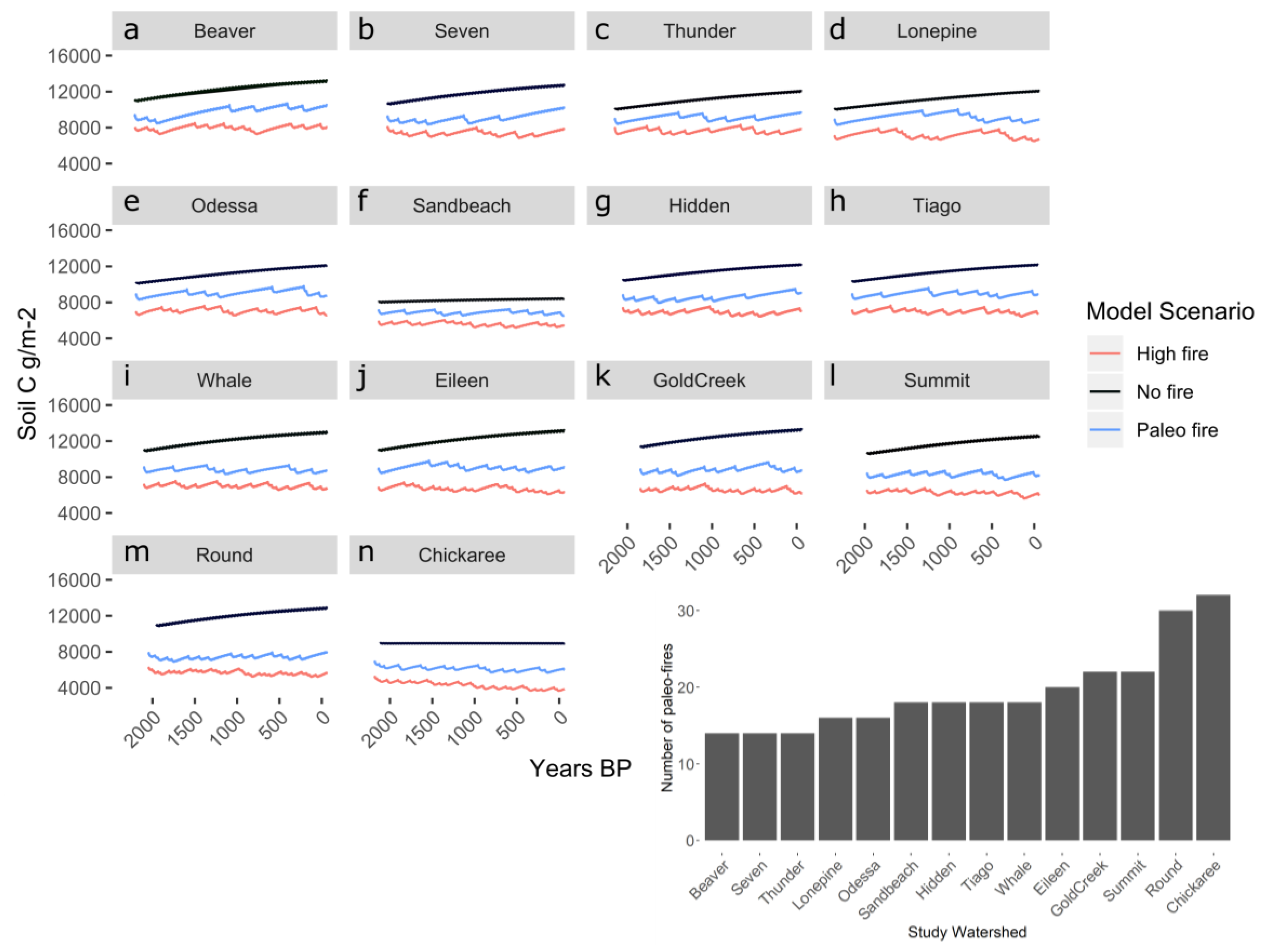
In all scenarios with fire, wildfire occurrence led to immediate and subsequent depletions in soil carbon (Figure 1); these small declines can be seen in the paleo-fire and high-fire simulations. Spikes in soil C show when fires occurred, as there is immediate loss of soil C (decline) following fire. A portion of soil carbon and nitrogen pools were lost and subsequently recovered at different rates. Consequently, higher fire frequencies over centennial time scales (shorter fire-free intervals) led to incremental reductions in carbon and nitrogen stocks (Figure 1, Figure 2, and Figure S5). Total ecosystem and soil carbon were lower at the end of the simulation period (i.e., in 2012) in simulations with high fire occurrence (e.g., at lakes with frequent paleo-fires and in high-fire scenarios compared to paleo-fire scenarios, Figures S6 and S7).
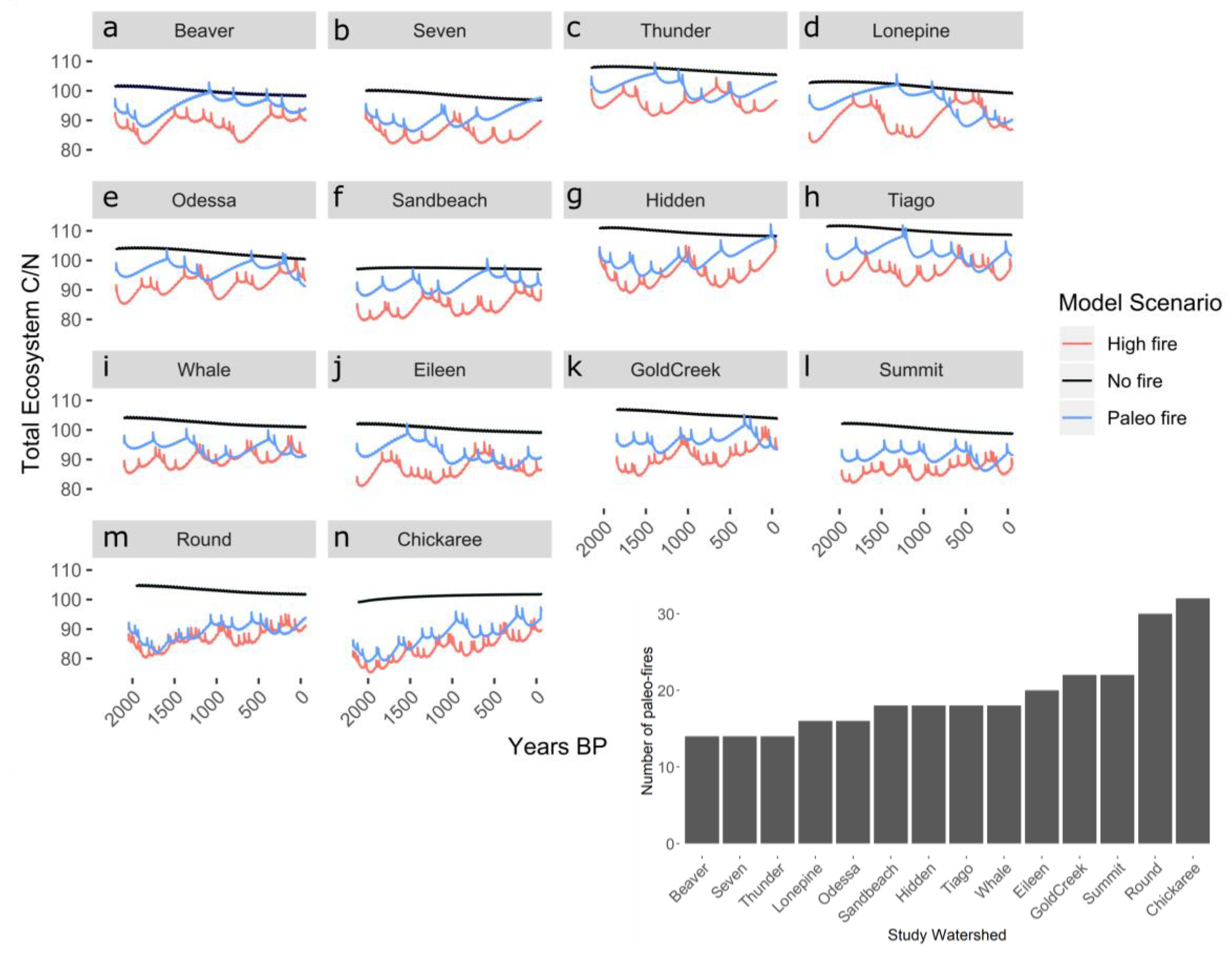
In addition to the changes in the soil carbon pool (Figure 1), the simulations also indicate substantial differences in ecosystem C:N among scenarios (Figure 2). Ecosystem C:N ratios for the no-fire scenario decline during the entire simulation period for all study sites, but fires substantially alter this trajectory. However, at each study site, even though soil carbon was lower for all high-fire scenarios than the paleo-fire scenarios, overall trajectories of ecosystem C:N were similar for high-fire and paleo-fire scenarios (Figure 2). The watersheds with high-frequency paleo-fire records (e.g., Chickaree and Round) had C:N ratios that were very similar for both high-fire and paleo-simulations (Figure 2).
In all the scenarios, fewer, or no, fires for more than a century led to slow but steady increases in both ecosystem C and N stocks. Post-fire recovery of different carbon and nitrogen pools varied based on fire frequency. The high-fire scenario lead to a decline of soil carbon across all sites, whereas the paleo-fire scenarios showed a range of soil carbon values, either decreasing or staying at equilibrium values of soil carbon.
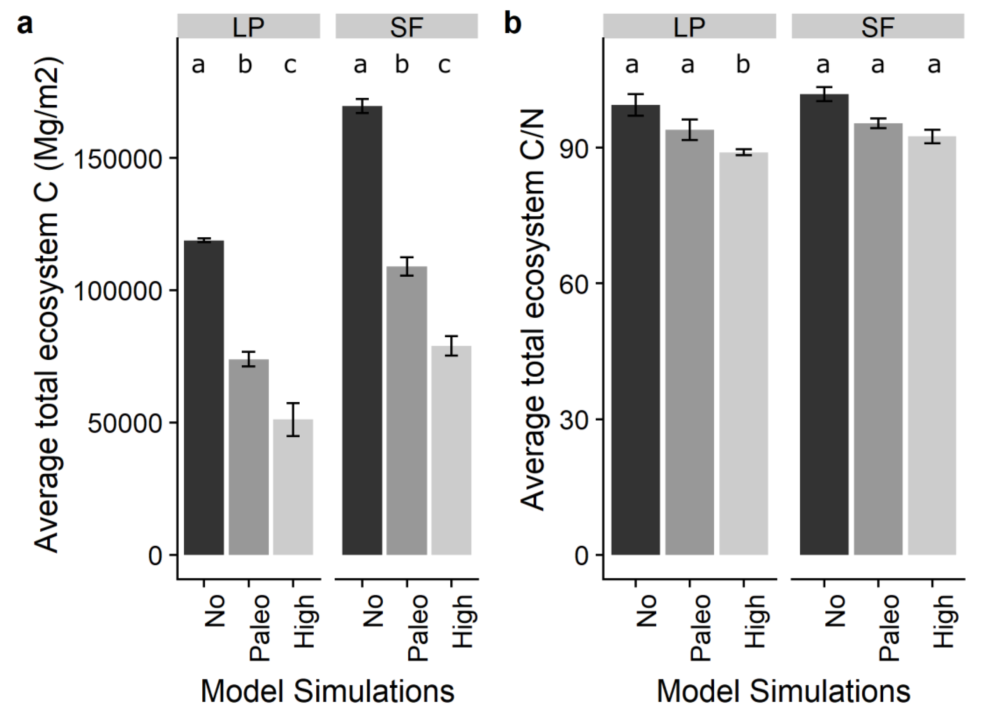
Comparing all study watersheds, regardless of forest type, final (end-of-simulation) total ecosystem carbon was significantly different between the three experimental simulations (Figure 3). No-fire scenarios had the highest values of ecosystem C stocks, followed by the paleo-fire and high-fire scenarios (F = 86.64, df = 2, p < 0.01). Final ecosystem C:N ratios were also significantly different between the three experimental simulations. No-fire scenarios had the highest C:N values, followed by paleo-fire and high-fire scenarios (F = 14.97, df = 2, p < 0.01).
3.2. Impacts of Forest Type on Carbon and Nitrogen Dynamics
Total ecosystem carbon was significantly lower in lodgepole forests than in spruce-fir forests (Figure 3a, dark grey bars, t = −2.62, df = 8, p = 0.03). C:N ratios were not significantly different between lodgepole and spruce-fir forests (Figure 3b, t = −1.05, df = 7, p = 0.32).
Total ecosystem carbon was significantly lower in the high-fire and paleo-fire scenarios compared to the no-fire scenarios in the spruce-fir forest watersheds (Figure 3a, F = 192, df = 2, p < 0.01), and in the lodgepole forest watersheds (Figure 3a, F = 33.18, df = 2, p < 0.01). C:N ratios were not significantly different in high-fire scenarios than in paleo-fire scenarios for spruce-fir forests (Figure 3b, F = 7.31, df = 2, p = 0.07). High-fire total ecosystem C:N ratios were significantly lower than paleo-fire scenarios in lodgepole pine forests (Figure 3b, F = 11.38, df = 2, p < 0.02).
3.3. Influence of Fire Frequency and Site Characteristics on C and N Dynamics
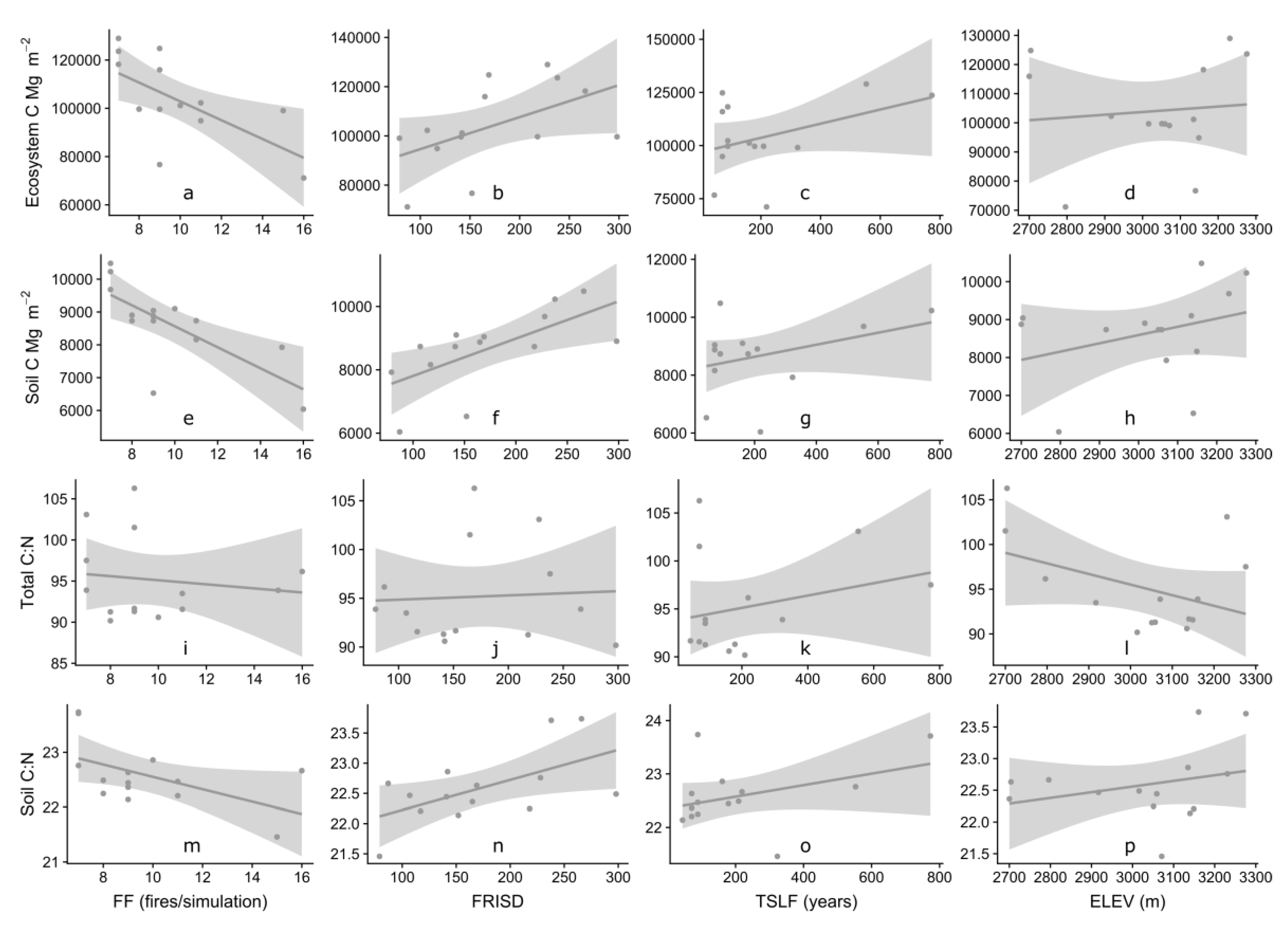
Influence of fire frequency (FF; number of fires over simulation length), fire return interval standard deviation (FRISD; the standard deviation of average time between fire events over simulation length), time since last fire (TSLF), and elevation (ELEV) were evaluated for their impact on model outputs from the paleo-fire scenario on all study sites. Total ecosystem and total soil carbon stocks were significantly lower in watersheds with higher paleo-fire occurrence than in other watersheds (Figure 4a,e, Table 3). Total C:N ratios did not significantly change with increase in FF, while soil C:N ratios were negatively correlated with fire frequency (Figure 4m, Table 3). Total ecosystem carbon, total soil carbon, and soil C:N ratios were highly correlated with increased FRISD (Figure 4b,f,n, Table 3). TSLF and ELEV were not correlated with carbon and nitrogen dynamics in the paleo-fire simulations (Figure 4, Table 3). There was no correlation relationship between FF and study site elevation (Figure S4), although there is a trend of decreasing FF with increasing elevation.
4. Discussion
Using DayCent forced with paleo-fire records, we found several new aspects of simulated carbon and nitrogen fluxes and stocks over the past 2000 years in subalpine forests. Ecosystem carbon trajectories were strongly dependent on fire frequency and timing of fire events. The length of fire-free intervals determined if a watershed gained or lost ecosystem carbon and nitrogen by the end of the simulation period. The occurrence of long fire-free periods led to ecosystem carbon gains whereas frequent fires led to large carbon losses. These results are broadly consistent with empirical work from boreal forests demonstrating that fire-free periods lead to substantial C sequestration in aboveground biomass and upper soil layers [7,48].
Overall, increases in fire frequency substantially decreased soil carbon across all sites over time (Figure 3a). These results have important biogeochemical implications for periods of elevated fire activity in the past [35], and in the future [4,7]. In this study, the repetition (through doubling the paleo-record fire history) of both fire occurrence and variability in the high-fire scenarios resulted in anew equilibria of overall lower carbon-carrying capacity compared to the paleo-fire scenarios. For example, in watersheds that had a long fire-free period at the end of the simulation, soil carbon increased for both the paleo and high-fire scenario (e.g., Seven Lake), but this increase is compressed in time and smaller in magnitude for the high-fire scenario. A long-term high-fire frequency may lower the overall carbon carrying capacity of subalpine forest, but this trend saturates (i.e., stops declining) as seen in a few of the watersheds with higher paleo fire frequency (e.g., Chickaree and Thunder). Reductions in total ecosystem carbon and soil carbon that result from increases in fire frequency may be predictive of future carbon storage in forested ecosystems in the current era of elevated wildfire activity [49], although many other factors contribute to soil carbon values including vegetation type and elevation [50].
High variability in fire return intervals (fire return interval standard deviation) significantly increased total and soil carbon, and raised soil C:N ratio, compared to low variability or no-fire scenarios. Long fire-free intervals in many high-variability simulations likely drove this set of results, because long fire-free periods led to a build-up of carbon and an increase in the soil C:N ratio. Although total ecosystem carbon stocks increased across the study sites in the no-fire scenario, nitrogen stocks also increased, leading to an overall decrease of C:N over time. In no-fire scenarios, nitrogen is being ‘locked up’ in biomass as it accumulates over millennia and not being lost to fire or post-fire impacts. In paleo-fire scenarios, soil C:N ratios decrease with increased fire frequency, which may be due to carbon lost during or after fires, and the return of bioavailable nitrogen to the ecosystem, thereby decreasing the soil C:N ratio. There have been few site-scale studies examining post-fire C:N ratios [51]; however, studies on small time scales (years to decades) and spatial scales (site-specific) may represent processes that differ from the drivers of patterns in our study, which examines C:N ratios across a study region (Southern Rockies) on a millennial timescale. During forest stand development, increases in total C usually occurs with increases in N [52]. In addition, forest floor C and N losses during prescribed fires can be large, and N volatilization during prescribed fires can be larger than N deposition in forests of the Sierra Nevada [53]. Post-fire C:N ratios can be indicative of the ability of the forest to recover, or availability of N for primary production to drive post-fire growth.
Both plant traits, such as foliar C:N, and potentially limiting nutrients, such as nitrogen, were found to be influenced by fire frequency. For example, variability in fire frequency led to high variability in ecosystem C:N ratios (Figure 2 and Figure 3) because of variation in the allocation of N among soil and plant pools. Doubling fire frequency (high-fire scenarios) lowered C:N ratios as compared to the paleo-fire scenarios. As paleo-fire frequency increases, the differences in C:N ratios between paleo and high-fire scenarios decreases. This suggests that there is a point of saturation with the amount of fire occurring, where the C:N ratios for the paleo- and high-fire scenarios are nearly equal (i.e., for Round and Chickaree Lakes) there is already a relatively high amount of fire occurring during the paleo-fire simulation. The lower C:N ratio also suggests that regrowth (or carbon carrying capacity) is not being limited by nutrient availability (nitrogen in DayCent) and is actually being limited by disturbance interval.
We found that no-fire simulations led to the highest total ecosystem carbon stocks for all the study sites. Some of the most carbon dense places in the world (e.g., tropical and temperate rainforests) [54] do not (or very rarely) naturally burn. Most tropical forest fires are human-caused [55] and these forests are not fire-adapted. Carbon carrying capacity is higher in places with no fire, although fire occurrence in fire-adapted ecosystems has other benefits in these ecosystems. Current trends of increased fire-frequency in fire-prone areas of the US [26] (including the Southern Rockies study region) may lead to lower carbon-carrying capacities, as shown by the decrease in total ecosystem carbon in the high-fire scenario (Figure 2). Further simulations with predictive and fully coupled ecosystem models will help elucidate the potential changes in forest carbon sink potential.
Forest type seems to play a role in total ecosystem carbon storage. Our distribution of forest types among study sites is not ideal for making broad comparisons (n = 2 for lodgepole pine and n = 12 for spruce-fir forests) and it would be a more robust analysis if more forest types had been represented equally. However, this study relied on previously collected paleo-fire reconstructions, of which there were 12 spruce-fir forests and two lodgepole pine forests. We parameterized model runs based on forest type because these species are different physiologically. Model output for the two forest types proved to be significantly different, making the results important to report.
A limitation of this study is the lack of paleoclimate forcing data in the DayCent simulations. Using paleoclimate forcing data would allow for the model scenarios to test the impact of climate, in addition to fire regime variability. However, because our fire events are completely prescribed, they are decoupled from climate in the model simulations. We cannot easily acquire the proper scale of paleoclimate data for these study locations, making these impacts beyond the capability of the current study. Rather than introduce the additional uncertainty of downscaled paleoclimate data (both temporal and spatial), we chose to use climate data that was more specific to each site (Daymet; nearest weather station). As fires are prescribed (not predicted based on climate or vegetation type), our study tested the impact of fire regime variability and fire occurrence variability on carbon and nitrogen dynamics. Paleoclimate data is at such a large timestep and coarse spatial resolutions that downscaling it to use in a daily-timestep model for individual study sites would mask any results that could be interpreted from it.
The biogeochemical model DayCent allowed for the exploration of how known past fire events affected forested watersheds in Colorado. However, DayCent is not currently coupled with a predictive fire, vegetation, or climate model. Because of this limitation of the model, DayCent cannot predict fire or vegetation changes that result from changing climate and disturbance regimes. The results here provide a benchmark for comparison in future research utilizing fully coupled ecosystem model that includes a dynamic vegetation component (e.g., DGVM ecosystem models) and a prognostic fire model (e.g., SPITFIRE [56]). Simulating Southern Rockies forests with a DGVM coupled with a climate and fire model will allow for predictions of C and N dynamics in forests with altered fire regimes under climate change.
Supplementary Materials
The following are available online at https://0-www-mdpi-com.brum.beds.ac.uk/2571-6255/2/4/58/s1, Figure S1: Study site locations in Colorado, USA. The northern sites are in the Medicine Bow-Routt National Forest and the southern sites are in the Rocky Mountain National Park. Figure S2: Soil carbon stocks over simulation lengths for paleo-fire (grey) simulations and equilibrium (black) simulations. Equilibrium simulations were run with the average fire return interval. Figure S3: Modeled soil carbon validation. Modeled soil carbon is not significantly different from collected soil carbon (data). The error bars represent standard errors. Figure S4: Fire frequency (number of fires over the length of the simulation period) by elevation (m). r2 = 0.1325, p = 0.20. Figure S5: Total ecosystem nitrogen over the simulation length for each scenario and each study. Figure S6: Difference between start and end soil C values for each study location and each simulation scenario. Figure S7: Difference between start and end total ecosystem C values for each study location and each simulation scenario. Table S1: Number of fires that were prescribed in both the paleo-fire scenario and high-fire scenario for each model simulation. Table S2: Field collection study sites. Data, including parameterization and calibration files, can be found in supporting documents.
Author Contributions
Conceptualization, K.J.B. and T.W.H.; methodology, K.J.B. and T.W.H.; validation, K.J.B. and T.W.H.; formal analysis, K.J.B. and T.W.H.; investigation, K.J.B. and T.W.H.; writing—original draft preparation, K.J.B., P.E.H., B.N.S., K.K.M. and T.W.H.; writing—review and editing, K.J.B., P.E.H., B.N.S., K.K.M. and T.W.H.
Funding
Kristina J. Bartowitz and Tara W. Hudiburg were funded by the National Science Foundation under award number DEB-1655183 and DMS-1520873. Philip E. Higuera was funded by the National Science Foundation under award number(s) DEB-1655121. Bryan N. Shuman was funded by the National Science Foundation under award number(s) DEB-1655189. Kendra K. McLauchlan was funded by the National Science Foundation under award number DEB-1655179. The authors declare no competing financial conflicts of interests or other affiliations with conflicts of interest with respect to the results of the paper.
Acknowledgments
We thank the Big Burns team for valuable discussions on these topics and assistance in the field. We also thank J. Stenzel for valuable fieldwork assistance.
Conflicts of Interest
The authors declare no conflict of interest.
References
- Le Quéré, C.; Andrew, R.M.; Friedlingstein, P.; Sitch, S.; Hauck, J.; Pongratz, J.; Pickers, P.A.; Korsbakken, J.I.; Peters, G.P.; Canadell, J.G.; et al. Global Carbon Budget 2018. Earth Syst. Sci. Data 2018, 10, 2141–2194. [Google Scholar] [CrossRef] [Green Version]
- Intergovernmental Panel on Climate Change IPCC. Part A: Global and Sectoral Aspects. In Climate Change 2014: Impacts, Adaptation, and Vulnerability; Contribution of Working Group II to the Fifth Assessment Report of the Intergovernmental Panel on Climate Change; Cambridge University Press: Cambridge, UK, 2014; pp. 1–32. [Google Scholar]
- Hudiburg, T.W.; Law, B.E.; Turner, D.P.; Campbell, J.L.; Donato, D.C.; Duane, M. Carbon dynamics of Oregon and Northern California forests and potential land-based carbon storage. Ecol. Appl. 2009, 19, 163–180. [Google Scholar] [CrossRef] [PubMed]
- Buotte, P.C.; Levis, S.; Law, B.E.; Hudiburg, T.W.; Rupp, D.E.; Kent, J.J. Near-future forest vulnerability to drought and fire varies across the western United States. Glob. Chang. Biol. 2019, 25, 290–303. [Google Scholar] [CrossRef] [PubMed] [Green Version]
- Schwalm, C.R.; Williams, C.A.; Schaefer, K.; Baldocchi, D.; Black, T.A.; Goldstein, A.H.; Law, B.E.; Oechel, W.C.; Scott, R.L. Reduction in carbon uptake during turn of the century drought in western North America. Nat. Geosci. 2012, 5, 551–556. [Google Scholar] [CrossRef] [Green Version]
- Hudiburg, T.W.; Higuera, P.E.; Hicke, J.A. Fire-regime variability impacts forest carbon dynamics for centuries to millennia. Biogeosciences 2017, 14, 3873–3882. [Google Scholar] [CrossRef] [Green Version]
- Kelly, R.; Genet, H.; McGuire, A.D.; Hu, F.S. Palaeodata-informed modelling of large carbon losses from recent burning of boreal forests. Nat. Clim. Chang. 2015, 6, 79–82. [Google Scholar] [CrossRef]
- Amiro, B.D.; Barr, A.G.; Barr, J.G.; Black, T.A.; Bracho, R.; Brown, M.; Chen, J.; Clark, K.L.; Davis, K.J.; Desai, A.R.; et al. Ecosystem carbon dioxide fluxes after disturbance in forests of North America. J. Geophys. Res. Biogeosci. 2010, 115. [Google Scholar] [CrossRef]
- Berner, L.T.; Law, B.E.; Meddens, A.J.; Hicke, J.A. Tree mortality from fires, bark beetles, and timber harvest during a hot and dry decade in the western United States (2003–2012). Environ. Res. Lett. 2017, 12, 065005. [Google Scholar] [CrossRef] [Green Version]
- Liang, S.; Hurteau, M.D.; Westerling, A.L. Potential decline in carbon carrying capacity under projected climate-wildfire interactions in the Sierra Nevada. Sci. Rep. 2017, 7, 2420. [Google Scholar] [CrossRef]
- Seidl, R.; Rammer, W.; Spies, T.A. Disturbance legacies increase the resilience of forest ecosystem structure, composition, and functioning. Ecol. Appl. 2014, 24, 2063–2077. [Google Scholar] [CrossRef] [Green Version]
- Turner, M.G.; Braziunas, K.H.; Hansen, W.D.; Harvey, B.J. Short-interval severe fire erodes the resilience of subalpine lodgepole pine forests. Proc. Natl. Acad. Sci. USA 2019, 116, 11319–11328. [Google Scholar] [CrossRef] [PubMed] [Green Version]
- Schoennagel, T.; Veblen, T.T.; Romme, W.H. The Interaction of Fire, Fuels, and Climate across Rocky Mountain Forests. Bioscience 2004, 54, 661–676. [Google Scholar] [CrossRef]
- Pausas, J.G.; Bradstock, R.A.; Keith, D.A.; Keeley, J.E.; Hoffman, W.; Kenny, B.; Lloret, F.; Trabaud, L. Plant functional traits in relation to fire in crown-fire ecosystems. Ecology 2004, 85, 1085–1100. [Google Scholar] [CrossRef] [Green Version]
- Clarke, P.J.; Lawes, M.J.; Murphy, B.P.; Russell-Smith, J.; Nano, C.E.M.; Bradstock, R.; Enright, N.J.; Fontaine, J.B.; Gosper, C.R.; Radford, I.; et al. A synthesis of postfire recovery traits of woody plants in Australian ecosystems. Sci. Total Environ. 2015, 534, 31–42. [Google Scholar] [CrossRef] [PubMed]
- Keeley, J.E.; Pausas, J.G.; Rundel, P.W.; Bond, W.J.; Bradstock, R.A. Fire as an evolutionary pressure shaping plant traits. Trends Plant Sci. 2011, 16, 406–411. [Google Scholar] [CrossRef] [PubMed] [Green Version]
- Poulos, H.; Barton, A.; Slingsby, J.; Bowman, D. Do Mixed Fire Regimes Shape Plant Flammability and Post-Fire Recovery Strategies? Fire 2018, 1, 39. [Google Scholar] [CrossRef] [Green Version]
- Archibald, S.; Hempson, G.P.; Lehmann, C. A unified framework for plant life-history strategies shaped by fire and herbivory. New Phytol. 2019. [Google Scholar] [CrossRef]
- Leys, B.; Higuera, P.E.; McLauchlan, K.K.; Dunnette, P.V. Wildfires and geochemical change in a subalpine forest over the past six millennia. Environ. Res. Lett. 2016, 11, 125003. [Google Scholar] [CrossRef]
- Pompeani, D.P.; McLauchlan, K.K.; Chileen, B.V.; Wolf, K.D.; Higuera, P.E. Variation of key elements in soils and plant tissues in subalpine forests of the northern Rocky Mountains, USA. Biogeosci. Discuss. 2018, 1–19. [Google Scholar] [CrossRef]
- Davis, K.T.; Dobrowski, S.Z.; Higuera, P.E.; Holden, Z.A.; Veblen, T.T.; Rother, M.T.; Parks, S.A.; Sala, A.; Maneta, M.P. Wildfires and climate change push low-elevation forests across a critical climate threshold for tree regeneration. Proc. Natl. Acad. Sci. USA 2019, 116, 6193–6198. [Google Scholar] [CrossRef] [Green Version]
- Stevens-Rumann, C.S.; Kemp, K.B.; Higuera, P.E.; Harvey, B.J.; Rother, M.T.; Donato, D.C.; Morgan, P.; Veblen, T.T. Evidence for declining forest resilience to wildfires under climate change. Ecol. Lett. 2018, 21, 243–252. [Google Scholar] [CrossRef] [PubMed]
- Abatzoglou, J.T.; Williams, A.P. Impact of anthropogenic climate change on wildfire across western US forests. Proc. Natl. Acad. Sci. USA 2016, 113, 11770–11775. [Google Scholar] [CrossRef] [PubMed] [Green Version]
- Balch, J.K.; Bradley, B.A.; Abatzoglou, J.T.; Nagy, R.C.; Fusco, E.J.; Mahood, A.L. Human-started wildfires expand the fire niche across the United States. Proc. Natl. Acad. Sci. USA 2017, 114, 2946–2951. [Google Scholar] [CrossRef] [Green Version]
- Littell, J.S.; Mckenzie, D.; Peterson, D.L.; Anthony, L. Climate and Wildfire Area Burned in Western U.S. Ecoprovinces, 1916–2003. Ecol. Appl. 2009, 19, 1003–1021. [Google Scholar] [CrossRef] [PubMed]
- Westerling, A.L.; Hidalgo, H.G.; Cayan, D.R.; Swetnam, T.W. Warming and earlier spring increase western US forest wildfire activity. Science 2006, 313, 940–943. [Google Scholar] [CrossRef] [PubMed] [Green Version]
- Littell, J.S.; Peterson, D.L.; Riley, K.L.; Liu, Y.; Luce, C.H. A review of the relationships between drought and forest fire in the United States. Glob. Chang. Biol. 2016, 22, 2353–2369. [Google Scholar] [CrossRef] [PubMed]
- Miller, J.D.; Safford, H.D.; Crimmins, M.; Thode, A.E. Quantitative evidence for increasing forest fire severity in the Sierra Nevada and southern Cascade Mountains, California and Nevada, USA. Ecosystems 2009, 12, 16–32. [Google Scholar] [CrossRef]
- Seidl, R.; Spies, T.A.; Peterson, D.L.; Stephens, S.L.; Hicke, J.A. Searching for resilience: Addressing the impacts of changing disturbance regimes on forest ecosystem services. J. Appl. Ecol. 2016, 53, 120–129. [Google Scholar] [CrossRef] [Green Version]
- Chapin, F.S., III; Woodwell, G.M.; Randerson, J.T.; Rastetter, E.B.; Lovett, G.M.; Baldocchi, D.D.; Clark, D.A.; Harmon, M.E.; Schimel, D.S.; Valentini, R.; et al. Reconciling carbon-cycle concepts, terminology, and methods. Ecosystems 2006, 9, 1041–1050. [Google Scholar] [CrossRef] [Green Version]
- Bonan, G.B.; Doney, S.C. Climate, ecosystems, and planetary futures: The challenge to predict life in Earth system models. Science 2018, 359, eaam8328. [Google Scholar] [CrossRef] [Green Version]
- Law, B.E.; Hudiburg, T.W.; Berner, L.T.; Kent, J.J.; Buotte, P.C.; Harmon, M.E. Land use strategies to mitigate climate change in carbon dense temperate forests. Proc. Natl. Acad. Sci. USA 2018, 115, 3663–3668. [Google Scholar] [CrossRef] [PubMed] [Green Version]
- Fisher, R.A.; Koven, C.D.; Anderegg, W.R.L.; Christoffersen, B.O.; Dietze, M.C.; Farrior, C.E.; Holm, J.A.; Hurtt, G.C.; Knox, R.G.; Lawrence, P.J.; et al. Vegetation demographics in Earth System Models: A review of progress and priorities. Glob. Chang. Biol. 2018, 24, 35–54. [Google Scholar] [CrossRef] [PubMed] [Green Version]
- Hantson, S.; Arneth, A.; Harrison, S.P.; Kelley, D.I.; Prentice, I.C.; Rabin, S.S.; Archibald, S.; Mouillot, F.; Arnold, S.R.; Artaxo, P.; et al. The status and challenge of global fire modelling. Biogeosciences 2016, 13, 3359–3375. [Google Scholar] [CrossRef] [Green Version]
- Calder, W.J.; Parker, D.; Stopka, C.J.; Jiménez-Moreno, G.; Shuman, B.N. Medieval warming initiated exceptionally large wildfire outbreaks in the Rocky Mountains. Proc. Natl. Acad. Sci. USA 2015, 112, 13261–13266. [Google Scholar] [CrossRef] [PubMed] [Green Version]
- Dunnette, P.V.; Higuera, P.E.; Mclauchlan, K.K.; Derr, K.M.; Briles, C.E.; Keefe, M.H. Biogeochemical impacts of wildfires over four millennia in a Rocky Mountain subalpine watershed. New Phytol. 2014, 203, 900–912. [Google Scholar] [CrossRef]
- Higuera, P.E.; Briles, C.E.; Whitlock, C. Fire-regime complacency and sensitivity to centennial through millennial-scale climate change in Rocky Mountain subalpine forests, Colorado, USA. J. Ecol. 2014, 102, 1429–1441. [Google Scholar] [CrossRef]
- Bai, E.; Houlton, B.Z. Coupled isotopic and process-based modeling of gaseous nitrogen losses from tropical rain forests. Glob. Biogeochem. Cycles 2009, 23, 1–10. [Google Scholar] [CrossRef]
- Hartman, M.D.; Baron, J.S.; Ojima, D.S. Application of a coupled ecosystem-chemical equilibrium model, DayCent-Chem, to stream and soil chemistry in a Rocky Mountain watershed. Ecol. Modell. 2007, 200, 493–510. [Google Scholar] [CrossRef]
- Savage, K.E.; Parton, W.J.; Davidson, E.A.; Trumbore, S.E.; Frey, S.D. Long-term changes in forest carbon under temperature and nitrogen amendments in a temperate northern hardwood forest. Glob. Chang. Biol. 2013, 19, 2389–2400. [Google Scholar] [CrossRef] [Green Version]
- Hengl, T.; De Jesus, J.M.; Heuvelink, G.B.M.; Gonzalez, M.R.; Kilibarda, M.; Blagotić, A.; Shangguan, W.; Wright, M.N.; Geng, X.; Bauer-Marschallinger, B.; et al. SoilGrids250m: Global gridded soil information based on machine learning. PLoS ONE 2017, 12, e0169748. [Google Scholar] [CrossRef] [Green Version]
- Stenzel, J.E.; Bartowitz, K.J.; Hartman, M.D.; Lutz, J.A.; Crystal, A.; Parton, W.J.; Hudiburg, T.W. Fixing a snag in carbon emissions estimates from wildfires. Glob. Chang. Biol. 2019. [Google Scholar] [CrossRef] [PubMed]
- Law, B.E.; Arkebauer, T.; Chen, J.; Campbell, J.L.; Sun, O.; Schwartz, M.; van Ingen, C.; Verma, S. Terrestrial Carbon Observations: Protocols for Vegetation Sampling and Data Submission; Global Terrestrial Observing System, FAO: Rome, Italy, 2008. [Google Scholar]
- Sampson, D.A.; Allen, H.L. Direct and indirect estimates of Leaf Area Index (LAI) for lodgepole and loblolly pine stands. Trees 1995, 9, 119–122. [Google Scholar] [CrossRef]
- Aplet, G.H.; Smith, F.W.; Laven, R.D. Stemwood Biomass and Production during Spruce-Fir Stand Development. J. Ecol. 1989, 77, 70–77. [Google Scholar] [CrossRef]
- Thornton, P.E.; Thornton, M.M.; Mayer, B.W.; Wilhelmi, N.; Wei, Y.; Devarakonda, R.; Cook, R. Daymet: Daily surface weather on a 1 km grid for North America, 1980–2008. Oak Ridge Natl. Lab. Distrib. Act. Arch. Cent. Biogeochem. Dyn. DAAC 2012. [Google Scholar] [CrossRef]
- R Core Team. A Language and Environment for Statistical Computing; R Foundation for Statistical Computing: Vienna, Austria, 2017. [Google Scholar]
- Brown, C.D.; Johnstone, J.F. How does increased fire frequency affect carbon loss from fire? A case study in the northern boreal forest. Int. J. Wildl. Fire 2011, 20, 829–837. [Google Scholar] [CrossRef]
- Law, B.E.; Waring, R.H. Carbon implications of current and future effects of drought, fire and management on Pacific Northwest forests. For. Ecol. Manag. 2015, 355, 4–14. [Google Scholar] [CrossRef] [Green Version]
- Jobbágy, E.G.; Jackson, R.B. The vertical distribution of soil organic carbon and its relation to climate and vegetation. Ecol. Appl. 2000, 10, 423–436. [Google Scholar] [CrossRef]
- Knicker, H. How does fire affect the nature and stability of soil organic nitrogen and carbon? A review. Biogeochemistry 2007, 85, 91–118. [Google Scholar] [CrossRef]
- Yang, Y.; Luo, Y.; Finzi, A.C. Carbon and nitrogen dynamics during forest stand development: A global synthesis. New Phytol. 2011, 190, 977–989. [Google Scholar] [CrossRef]
- Caldwell, T.G.; Johnson, D.W.; Miller, W.W.; Qualls, R.G. Forest floor carbon and nitrogen losses due to prescription fire. Soil Sci. Soc. Am. J. 2002, 66, 262–267. [Google Scholar] [CrossRef]
- Pan, Y.; Birdsey, R.A.; Fang, J.; Houghton, R.; Kauppi, P.E.; Kurz, W.A. A Large and Persistent Carbon Sink in the World’s Forests. Science 2011, 333, 988–993. [Google Scholar] [CrossRef] [PubMed] [Green Version]
- Juárez-Orozco, S.M.; Siebe, C.; Fernández y Fernández, D. Causes and Effects of Forest Fires in Tropical Rainforests: A Bibliometric Approach. Trop. Conserv. Sci. 2017, 10, 194008291773720. [Google Scholar] [CrossRef]
- Lasslop, G.; Thonicke, K.; Kloster, S. SPITFIRE within the MPI Earth system model: Model development and evaluation. J. Adv. Model. Earth Syst. 2014, 6, 740–755. [Google Scholar] [CrossRef]
Figure 1.
Soil carbon stocks over the simulation period for each watershed. Plots are ordered from low (a) to high (n) paleo-fire frequency (i.e., Beaver has the lowest fire frequency and Chickaree has the highest), as shown by the bar graph inset. The bar graph inset shows the number of paleo-record fires during the simulation length of each scenario for that study location.

Figure 2.
Simulated total (all aboveground and belowground biomass and soil pools) C:N ratio over simulation length. The plots are ordered from low (a) to high (n) paleo-fire frequency (i.e., Beaver has the lowest fire frequency and Chickaree has the highest), as shown by the bar graph inset. The bar graph inset shows the number of paleo-record fires during the simulation length of each scenario for that study location.

Figure 3.
Forest-type variation in final ecosystem carbon and C:N ratios by model scenario. (a) Forest-type final (end of simulation) ecosystem carbon by forest types, lodgepole pine (LP) and spruce-fir (SF). (b) Forest type final (end of simulation) C:N by lodgepole pine and spruce-fir forests. The error bars represent the standard error in each scenario-forest type combination.

Figure 4.
Variation in total ecosystem carbon (Mg m−2), soil carbon (Mg m−2), total C:N ratios, and soil C:N ratios in by fire frequency (number of fires over the simulation period, FF), fire return interval standard deviation (FRISD), time since last fire (TSLF), and elevation (m, ELEV). Figure panels are labeled (a)–(p) to refer to panels in text.


Table 1.
Study sites in the Southern Rocky Mountains. Sub-regions include Rocky Mountain National Park (RMNP) and Medicine Bow-Routt National Forest (MBR-NF).
Table 1.
Study sites in the Southern Rocky Mountains. Sub-regions include Rocky Mountain National Park (RMNP) and Medicine Bow-Routt National Forest (MBR-NF).
| Study Site | Lat., Long. | Sub-Region | Forest Type | Elevation (m) | Mean FRI (yr) [SD] | Simulation Length |
|---|---|---|---|---|---|---|
| Eileen | 40.902, −106.674 | MBR-NF | Spruce-fir | 3135 | 220 [142] | 2197 |
| Seven | 40.896, −106.682 | MBR-NF | Upper-treeline spruce-fir | 3276 | 298 [238] | 2089 |
| Gold Creek | 40.782, −106.678 | MBR-NF | Spruce-fir | 2917 | 174 [107] | 1909 |
| Hidden | 40.771, −106.827 | MBR-NF | Spruce-fir | 2704 | 234 [169] | 2107 |
| Beaver | 40.753, −106.687 | MBR-NF | Spruce-fir | 3161 | 283 [266] | 1981 |
| Tiago | 40.579, −106.613 | MBR-NF | Spruce-fir | 2700 | 244 [165] | 2197 |
| Whale | 40.556, −106.675 | MBR-NF | Spruce-fir | 3059 | 240 [141] | 2161 |
| Summit | 40.545, −106.682 | MBR-NF | Upper-treeline spruce-fir | 3149 | 185 [117] | 2035 |
| Round | 40.473, −106.663 | MBR-NF | Spruce-fir | 3071 | 134 [79] | 2107 |
| Chickaree | 40.334, −105.840 | RMNP | Lodgepole | 2796 | 136 [87] | 2180 |
| Odessa | 40.330, −105.685 | RMNP | Spruce-fir | 3051 | 281 [218] | 2251 |
| Lonepine | 40.232, −105.730 | RMNP | Spruce-fir | 3016 | 302 [298] | 2416 |
| Thunder | 40.221, −105.647 | RMNP | Spruce-fir | 3231 | 315 [228] | 2206 |
| Sandbeach | 40.218, −105.601 | RMNP | Lodgepole | 3140 | 243 [152] | 2191 |
Table 2.
Model scenario descriptions.
| Scenario | Description | Climate |
|---|---|---|
| Equilibrium | Fire prescribed using the mean fire return interval (FRI) of the paleo-fire record | Modern-recycled |
| Paleo-fire | Fire prescribed using site-specific paleo-fire record | Modern-recycled |
| High-fire | Fire prescribed by doubling the site-specific paleo-fire record; e.g., fire-history is repeated twice in the 2000-year record | Modern-recycled |
| No-fire | No disturbance/fire | Modern-recycled |
Table 3.
Correlation coefficients comparing paleo-fire scenarios in all the study sites. Relationships determined between total ecosystem carbon (TEC), soil carbon (Soil C), total C:N ratios, and soil C:N ratios in spruce-fir forests by fire frequency (number of fires over the simulation period), fire return interval standard deviation, time since last fire, and elevation (m). The bold values denote significant linear correlations.
| FF | FRISD | TSLF | ELEV | ||
|---|---|---|---|---|---|
| TEC | r2 | 0.4043 | 0.2671 | 0.1696 | 0.0101 |
| Soil C | r2 | 0.5293 | 0.4259 | 0.0128 | 0.176 |
| Total C:N | r2 | 0.0182 | 0.0033 | 0.0704 | 0.1822 |
| Soil C:N | r2 | 0.2835 | 0.3278 | 0.1489 | 0.0779 |
© 2019 by the authors. Licensee MDPI, Basel, Switzerland. This article is an open access article distributed under the terms and conditions of the Creative Commons Attribution (CC BY) license (http://creativecommons.org/licenses/by/4.0/).
Share and Cite
MDPI and ACS Style
Bartowitz, K.J.; Higuera, P.E.; Shuman, B.N.; McLauchlan, K.K.; Hudiburg, T.W. Post-Fire Carbon Dynamics in Subalpine Forests of the Rocky Mountains. Fire 2019, 2, 58. https://0-doi-org.brum.beds.ac.uk/10.3390/fire2040058
AMA Style
Bartowitz KJ, Higuera PE, Shuman BN, McLauchlan KK, Hudiburg TW. Post-Fire Carbon Dynamics in Subalpine Forests of the Rocky Mountains. Fire. 2019; 2(4):58. https://0-doi-org.brum.beds.ac.uk/10.3390/fire2040058
Chicago/Turabian StyleBartowitz, Kristina J., Philip E. Higuera, Bryan N. Shuman, Kendra K. McLauchlan, and Tara W. Hudiburg. 2019. "Post-Fire Carbon Dynamics in Subalpine Forests of the Rocky Mountains" Fire 2, no. 4: 58. https://0-doi-org.brum.beds.ac.uk/10.3390/fire2040058